A GPU Implementation of the Inverse Fast Multipole Method
for Multi-Bistatic Imaging Applications
Luis E. Tirado1, Galia Ghazi1, Yuri ´Alvarez-Lopez2, Fernando Las-Heras2, and Jos´e ´A. Martinez-Lorenzo1, *
Abstract—This paper describes a parallel implementation of the Inverse Fast Multipole Method (IFMM) for multi-bistatic imaging configurations. NVIDIAs Compute Unified Device Architecture (CUDA) is used to parallelize and accelerate the imaging algorithm in a Graphics Processing Unit (GPU). The algorithm is validated with synthetic data generated by the Modified Equivalent Current Approximation (MECA) method and experimental data collected by a Frequency-Modulated Continuous Wave (FMCW) radar system operating in the 70–77 GHz frequency band. The presented results show that the IFMM implementation using the CUDA platform is effective at significantly reducing the algorithm computational time, providing a 300X speedup when compared to the single core OpenMP version of the algorithm.
1. INTRODUCTION
The use of millimeter wave imaging technology has been widely adopted to detect security threats, like Improvised Explosive Devices (IED), in airport checkpoints [1–6]. The images produced by such systems are often generated by backpropagating the scattered field in order to recover the reflectivity. There are two main requirements in electromagnetic imaging: fast calculation of the images, and accuracy. In general, reducing the calculation time requires considering free-space backpropagation models that might not be accurate at all (especially if the scattered field is acquired in the near field region). As a trade-off between accuracy and calculation time, acceleration schemes based on the Fast Multipole Method (FMM) [7, 8] have been developed.
The FMM is a forward operator that has been widely used in electromagnetics to enable fast calculation of the radiated field given the electromagnetic sources without jeopardizing result accuracy. It can be used in inverse problems (e.g., antenna diagnostics) based on iterative schemes that minimize a cost function [9, 10] to speed-up forward operations at each iteration. However, iterative schemes in inverse problems are still time-consuming if compared to the use of inverse operators. For this reason, an inverse operator derived from the FMM, the Inverse Fast Multipole Method (IFMM) has been presented in [11, 12] applied to inverse scattering and imaging problems.
The current implementation of IFMM using CPUs is computationally intensive when being evaluated at multiple frequencies and observation points for multiple transmitter and receiver configurations. Taking into account that the FMM has been efficiently implemented in Graphics Processing Units (GPUs) for efficient analysis of electromagnetic scattering problems [13] and acoustics [14], it is proposed to follow a similar methodology for the inverse operator, the IFMM, so that the computationally intensive parts of the IFMM code can be evaluated to the same accuracy at higher speeds by using a GPU.
Received 10 February 2017, Accepted 22 June 2017, Scheduled 18 July 2017 * Corresponding author: Jose Angel Martinez-Lorenzo ([email protected]).
1 Department of Electrical Engineering, Northeastern University, Boston, MA 02115, USA.2Department of Electrical Engineering,
Parallelization using GPUs is desired for the IFMM algorithm given that it can be used as an image reconstruction algorithm in a mm-wave concealed threat detection system. Solving this problem and generating real-time images is extremely important for a deployable system, including those operating in high-capacity mode [15–20]. The Department of Homeland Security (DHS), through its mission of preventing terrorism and enhancing security, requires a high throughput, non-invasive, accurate, and quick detection of person-borne threats in highly secure areas [1–3, 5, 6]. For this reason, it is essential to be able to process the scattered fields from the person under test into an accurate reconstruction as fast as possible. In this paper, the acceleration of the IFMM utilizing a GPU for different configurations of transmitter and receivers is presented and experimentally validated for a multi-bistatic radar configuration. The work is divided as follows: Section 2 gives an IFMM overview, Section 3 describes the GPU architecture and approaches used to speed up the IFMM code, while Section 4 details the performance of the algorithm with both simulated and measured data.
2. IFMM OVERVIEW
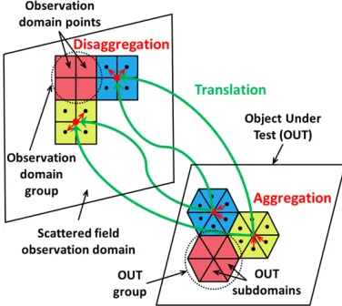
The IFMM algorithm is an inverse scattering technique [11], which may be used to reconstruct support and constitutive parameters of the object under test (OUT) from the acquired scattered field. The algorithm is based on backpropagating the scattered fields from the observation domain into the reconstruction or imaging domain to recover the reflectivity. The IFMM is derived from inverting a forward operator, the FMM. There are three IFMM operators: aggregation (1), translation (2), and disaggregation (3).
The first operator assumes that the scattered field,Em(q) (wheremand nindicate the measurement
and polarization indexes), can be locally approximated as a plane wave. For this goal, the scattered field observation groups mobs are defined. The phase-shift between the observation pointrm and the center
of the mobs-th observation group, Cmobs is defined as e+jk0(rm−Cmobs). Similarly, the disaggregation
operator assumes that the reflectivity, sometimes defined as equivalent currents, [11], Jn(p) (where n
and p indicate the current and polarization index respectively in a cubic sub-domain ΔVn) can be locally approximated as a plane wave within the source groups, nsource. The phase-shift between the center of the cubic sub-domain rn and the center of the nsource-th source group, Cnsource is defined as
e+jk0(Cnsource−rn).
Finally, the translation operator backpropagates the field from the center of the observation groups
Cmobsto the center of the source groupsCnsource, by means of a spherical wave expansion. It can be proved
that if the distance between the observation and source groups meets the far field criteria, the main contribution comes from the unit vector ˆkmobs,nsource, with the same direction asCmobs−Cnsource [7, 8]. In
the case of scattering problems, the far field criteria is fulfilled in most of the cases for all observation and source groups combinations, as explained in [11]. The indexesp, q= 1,2,3 in Eqs. (1)–(3) subsequently designate x,y, and z polarization for the following IFMM operators:
iA(mp)obs,nsource = C0· 3 q=1 Mmobs m=1
Km(p,qobs),nsourcee+jk0(rm−Cmobs)·ˆkmobs,nsource ·E(q)
m
(1)
iTm(pobs) ,nsource = iAm(p)obs,nsource ·4πjk0Cmobs−Cnsourcee+jk0|Cmobs−Cnsource| (2)
Jn(p) =
Mobs
mobs=1
e+jk0(Cnsource−rn)·kˆmobs,nsource ·
iTm(pobs) ,nsource·ΔVn, (3)
where Cmobs−Cnsource is the distance from the center of the mobs-th observation group Cmobs to the
center of the nsource-th source group Cnsource. The K
(p,q)
mobs,nsource dyadic term is defined and described
in [11], C0 = −η(k0/4π)2, η is the wave impedance, and the indexes in the previous equations are defined as follows [11]:
m= 1, . . . , Mmobs n= 1, . . . , Nsource (5)
rm ∈Mmobs Jn(p), rn,ΔVn ∈Nnsource, (6)
whereM is the number of observation points,Mmobs the number of elements in themobs-th observation
group, Mobs the number of observation groups, N the number of source points, Nnsource the number
of elements in the nsource-th source group, and Nsource the number of source groups. A graphic representation of the IFMM algorithm can be seen in Fig. 1.
Figure 1. IFMM scattered field observation and reconstruction (OUT) domains.
As explained in [11], the use of plane wave and spherical wave expansions is more accurate than the free-space backpropagation approach used in conventional SAR imaging (that can be speed up using Inverse Fast Fourier Transforms).
Concerning FMM and IFMM implementation, there is an important difference mainly due to the kind of problem (forward/inverse) where these acceleration schemes are used. FMM has been mostly used in forward scattering problems [7, 8], where the presence of near-field groups (i.e., observation and source groups adjacent to each other) requires the use of conventional MoM. Besides, if the far field distance is not met for a pair of observation-source groups, the translation operator, which is based on an spherical wave expansion, limits FMM speedup. This results in a more complex GPU implementation. IFMM is applied in inverse problems [11, 12], where in the majority of the cases the observation and source domains are physically different (as observed in Fig. 1), so the far field condition for each pair of observation-source groups is fulfilled. Thanks to this the translation operator can be reduced to a single spherical wave mode, which simplifies GPU implementation of IFMM, as it will be described in Section 3.
3. GPU IMPLEMENTATION DETAILS 3.1. Kepler CUDA Architecture
and other EUs in the SMX execute corresponding thread instructions. A challenge in implementing the IFMM on NVIDIA CUDA enabled GPUs is to make the most effective use of the platforms resources.
3.2. IFMM CUDA C Implementation
An existing and validated OpenMP version of the IFMM code was used to implement the CUDA C version. In the OpenMP IFMM version, the aggregation, translation, and disaggregation operations in Eqs. (1)–(3) are done via nested loops.
An initial version of the CUDA code used a 1D kernel for the aggregation operation and a separate 2D kernel for the translation operation. However, because the 1D kernel’s inner loop iterated over
Mobs Mmobs, a lesser amount of parallelism was exploited. Therefore, the execution time was slower.
The optimized approach computes the aggregation and translation steps described in Eqs. (1), (2) jointly, which avoids delays associated with additional kernel launches [22].
The disaggregation step from Eq. (3) is performed as a separate kernel. In its initial version, the disaggregation kernel used 2D indexing elements which corresponded to Nsource and Nnsource. This
kernel was launched with max(nsource) threads. Given the number of elements in each nsource group can vary, some launched threads can terminate without doing work due to being out of bounds. These terminated threads consume GPU resources that would otherwise be expended on threads that perform computations, thus increasing the overall execution time. The optimized disaggregation kernel uses 1D indexing based onN, the total number of source points, to avoid this issue.
A further optimization involves loading the 2D input variables into GPU memory as 1D flattened arrays in row-major format. This allows concurrent threads to simultaneously access adjacent memory addresses within the physical GPU memory. In this way, the GPU hardware is able to combine memory accesses which increases effective memory bandwidth [23]. Additionally, accessing data from 1D arrays is faster, as it avoids the cost of global memory reads associated with pointer indirections.
The IFMM aggregation/translation and disaggregation kernels are launched with 256 threads per thread block in order to ensure a fast execution time. For both kernels, the occupancy of each multiprocessor is limited by the number of registers used by the kernels. In an attempt to increase occupancy, both kernels were launched with a larger number of threads per block given the input data sets detailed in Section 4. However, given that these kernels are compute-bound, this approach results in the same or a slower execution time [24].
The output of the optimized aggregation and translation kernel is anMobs×Nsource array, so it is advantageous to arrange the 256 threads in each thread block into a 16×16 2D grid to take advantage
of CUDA’s grid structure [25]. Each thread in the kernel calculates a 2D index pair as follows:
xIdx=blockDim.x∗blockIdx.x+threadIdx.x (7)
yIdx=blockDim.y∗blockIdx.y+threadIdx.y (8) where threadIdx.x and threadIdx.y vary from [0, 15], and blockDim.x=blockDim.y=16. Each thread iterates over Mmobs, the number of elements of each observation group, to calculate one element of
the output matrix. For the aggregation/translation kernel, the thread block dimensionsblockIdx.x and blockIdx.y vary from [0, nR−1] and [0, nC−1], respectively.
The optimized disaggregation kernel arranges the 256 threads within each thread block in 1D, such that only Eq. (7) is used to index each thread. Thus, threadIdx.x varies from [0,255] and
blockDim.x = 256. This kernel launches N threads that iterate over Mobs, each of which computes
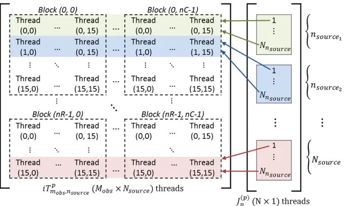
then-th equivalent current utilizing the output of the combined aggregation/translation kernel. Fig. 2 shows the arrangement of threads and blocks used to compute theiT(pmobs,nsource) and Jn(p) arrays. Each source point within a specific source group in the disaggregation kernel utilizes one column of data from the matrix computed by the aggregation/translation kernel.
For the CUDA version of the IFMM code, the kernels are batched consecutively, each set adding the results for the currentsJn(p)over the multiple processed frequencies. For example, processing a data-set with 32 frequencies means that 64 kernels will be executed−32 for the aggregation/disaggregation and 32 for the disaggregation operation. The process is summarized in the following pseudo-code:
For frequency from 1 to Fn:
(i) Launch 2D aggregation/translation kernel withMobs×Nsource threads, divided intonC×nRthread blocks. Each thread:
(a) Operates on a unique observation/source group.
(b) Iterates over Mmobs and computes vector rm−Cmobs and the scalar/complex products of Eq.
(1).
(c) Keeps result in GPU memory and uses it to calculate products of Eq. (2).
Output:iTm(pobs) ,nsource, an Mobs×Nsource array.
(ii) Launch 1D disaggregation kernel withN threads divided intonR thread blocks. Each thread: (a) Determines which source group the current source belongs to and computes vectorCnsource−rn.
(b) Iterates over Mobs and performs scalar/complex products in Eq. (3) using iTm(pobs) ,nsource and
accumulates their sum.
Output: Jn(p),N currents, matching to each source point. (iii) Keep a cumulative sum for each of the N currents.
End
4. APPLICATION EXAMPLES
The validation examples in this work were conducted with the CUDA IFMM code using a single workstation 3.4 GHz IntelR CoreTM i7-4930K hexa-core CPU with an NVIDIA GeForceR GTX Titan Black GPU with 6 GB of GDDR5 VRAM connected via a PCI-E 3.0×16 interface. This GPU contains 2880 CUDA cores, running at a base clock of 967 MHz. The IFMM OpenMP and CUDA codes were compiled with GCC/G++ 4.6.4. The CUDA 5.5 toolkit was used, and codes were profiled under 64-bit Ubuntu 14.04 with NVIDIA 337 drivers.
4.1. Simulation-Based Experiments
For performance tests, two data sets spanning the 70–77 GHz frequency range with varying input parameters are used. These sets (Experiment 1 & 2) use a tessellated model of the human body, composed of 9320 facets, as the object under test (OUT). The transmitting and receiving arrays are located 1.5m away from the body. The scattered electric field dataEm(q) in Eq. (1) is calculated via the MECA method [27]. In Experiment 1, receivers are arranged every λ/2 in a 1.5 m×1.5 m grid and 4 transmitters are employed at the grid corners. In Experiment 2, 1538 receivers are distributed into 2 horizontal lines, with the transmitters in a vertical line, once again arranged with a λ/2 spacing. The geometries for the experiments are shown in Figs. 3(a) and 3(b). The position of the transmitters and receivers in these figures is denoted by (Tx, Ty, Tz) and (Rx, Ry, Rz), respectively. Bx, By, and Bz denote the size of the minimum box enclosing the OUT (human body). For both experiments, the human body is discretized into 116 slices in the Z-direction, (0.05 m to 1.775 m) each of which is generated
(a) (b)
Figure 3. IFMM experiment geometry sketches. (a) Sketch of geometry for IFMM Experiment 1. (b) Sketch of geometry for IFMM Experiment 2.
(a) (b)
by the IFMM code for every transmitter. Each 687×129 pixels slice spans X = [−0.67 m 0.67 m] and
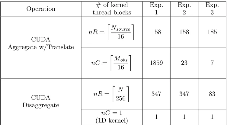
Y = [1.325 m 1.575 m]. The contributions for each transmitter are added non-coherently to produce the final reconstruction. Figs. 4(a) and 4(b) show the IFMM reconstruction results overlaid over the human body model for Experiments 1 and 2, respectively. Despite the different receiver/transmitter configurations, both methods produce similar images given the array geometry correspondence [28]. The nR and nC values for each of the IFMM reconstructions are listed in Table 1. Table 2 lists the IFMM input parameters used in evaluating the two simulation-based examples, as well as a measured data reconstruction.
Table 1. IFMM kernel launch parameters.
Operation # of kernel
thread blocks Exp. 1 Exp. 2 Exp. 3 CUDA Aggregate w/Translate nR= Nsource 16
158 158 185
nC=
Mobs 16
1859 23 7
CUDA Disaggregate nR= N 256
347 347 83
nC = 1
(1D kernel) 1 1 1
Table 2. IFMM input parameters per slice.
Parameters Exp. 1 — Simul. Exp. 2 — Simul. Exp. 3 — Meas.
M (obs. points) 591361 1538 451
N (source points) 88623 88623 21115
Mobs 29736 354 101
Nsource 2528 2528 2945
# of frequencies 32 32 731
max(Nnsource) 45 45 12
max(Mmobs) 25 5 5
4.2. Measurement-Based Experiments
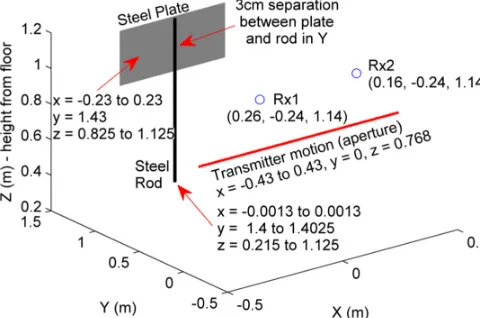
The third IFMM data set (Experiment 3) was collected with the 70–77 GHz Radar Front End (RFE) Model 8300 developed by the company HXI [29]. The data was collected by two receivers, indicated by
Figure 5. Sketch of geometry for measured data IFMM Experiment 3.
Figure 6. Top down view of steel plate and rod for Experiment 3.
21115 pixels are grouped into 2945 source groups — see the fourth column in Table 2. The scattered data is observed at 451 positions, which are grouped into 101 observation groups. Fig. 7 presents 2D images of the OUT, at thez= 0.954m plane, when the imaging is performed using the field measured by only the first receiver, by only the second receiver, and by both receivers.
4.3. Performance Evaluation
Table 3 shows the timing figures of the IFMM OpenMP implementation with 12 threads against the GTX Titan Black GPU CUDA code. The speedup factor of IFMM on the GPU versus the CPU counterpart is largely tied to the number of kernel thread blocks launched by the different data sets. For a larger amount of blocks used, the speedup is maximized, given that a larger level of parallelism is exploited. The IFMM CUDA code on the GTX Titan Black, which generates exactly the same image as the C-based version is able to achieve for Experiments 1, 2, and 3, respectively, the following speedups: 36X, 41X, and 20X, when compared to the OpenMP 12-core CPU version of the code; and 267X, 308X, and 157X, when compared to the 1-core CPU version of the code. Concerning numerical precision, results provided by CPU and GPU implementations were compared; the maximum normalized root mean square error observed for the experiments is below 1e-16.
Table 3. IFMM computation times per slice and transmitter.
IFMM modality
Time (ms)
Exp. 1 Exp. 2 Exp. 3
CUDA GPU 378 34879 1301
12-core CPU 13809 1462263 27215
Figure 7. Experiment 3 Reconstructed images: receiver 1 (top), receiver 2 (center), and non-coherent combination of both receivers (bottom). Normalized reflectivity, in dB.
5. CONCLUSION
This paper describes a CUDA implementation of the multi-static IFMM code, which has the potential to be used for real-time imaging of security threats. The performance of the OpenMP-based and the CUDA-based versions of the IFMM code has been evaluated using both synthetic and experimental datasets. In both cases, the CUDA-based version of the algorithm outperforms the OpenMP-based version, in terms of computational cost, without degrading the quality of the reconstructed image. The extension of the IFMM to operate with multiple levels, as it is often done by Multi-Level Fast Multipole Algorithms, will be studied in our future work.
ACKNOWLEDGMENT
This material is based upon work supported by the Science and Technology Directorate, U.S. Department of Homeland Security, Award No. 2013-ST-061-ED0001; by the “Ministerio de Econom´ıa y Competitividad” of Spain under project TEC2014-54005P (MIRIIEM); and by the “Gobierno del Principado de Asturias” under project GRUPIN14-114.
REFERENCES
1. Sheen, D., D. McMakin, and T. Hall, “Three-dimensional millimeter-wave imaging for concealed weapon detection,”IEEE Transactions on Microwave Theory and Techniques, Vol. 49, No. 9, 1581– 1592, 2001.
3. Martinez-Lorenzo, J. A., F. Quivira, and C. M. Rappaport, “SAR imaging of suicide bombers wearing concealed explosive threats,” Progress In Electromagnetics Research, Vol. 125, 255–272, 2012.
4. Alvarez, Y., B. Gonzalez-Valdes, J. Martinez Lorenzo, F. Las-Heras, and C. Rappaport, “3d whole body imaging for detecting explosive-related threats,” IEEE Transactions on Antennas and Propagation, Vol. 60, No. 9, 4453–4458, 2012.
5. Gonzalez-Valdes, B., Y. Alvarez, Y. Rodriguez-Vaqueiro, A. Arboleya-Arboleya, A. Garcia-Pino, C. M. Rappaport, F. Las-Heras, and J. A. Martinez-Lorenzo, “Millimeter wave imaging architecture for on-the-move whole body imaging,”IEEE Transactions on Antennas and Propagation, Vol. 64, No. 6, 2328–2338, Jun. 2016.
6. Gonzalez-Valdes, B., C. Rappaport, J. A. M. Lorenzo, Y. Alvarez, and F. Las-Heras, “Imaging effectiveness of multistatic radar for human body imaging,” 2015 IEEE International Symposium on Antennas and Propagation USNC/URSI National Radio Science Meeting, 681–682, Jul. 2015. 7. Coifman, R., V. Rokhlin, and S. Wandzura, “The fast multipole method for the wave equation:
a pedestrian prescription,” IEEE Antennas and Propagation Magazine, Vol. 35, No. 3, 7–12, Jun. 1993.
8. Darve, E., “The fast multipole method: Numerical implementation,” Journal
of Computational Physics, Vol. 160, No. 1, 195–240, 2000, [Online], Available: http://www.sciencedirect.com/science/article/pii/S0021999100964519.
9. Eibert, T. F. and C. H. Schmidt, “Multilevel fast multipole accelerated inverse equivalent current method employing rao-wilton-glisson discretization of electric and magnetic surface currents,”IEEE Transactions on Antennas and Propagation, Vol. 57, No. 4, 1178–1185, Apr. 2009.
10. Alvarez-Lopez, Y., F. Las-Heras, M. R. Pino, and J. A. Lopez, “Acceleration of the sources reconstruction method via the fast multipole method,” 2008 IEEE Antennas and Propagation Society International Symposium, 1–4, Jul. 2008.
11. Alvarez, Y., J. A. Martinez-Lorenzo, F. Las-Heras, and C. M. Rappaport, “An inverse fast multipole method for geometry reconstruction using scattered field information,” IEEE Transactions on Antennas and Propagation, Vol. 60, No. 7, 3351–3360, 2012.
12. Schnattinger, G. and T. F. Eibert, “Solution of the vectorial 3d inverse source problem by adjoint near-field fast multipole translations,” Proceedings of the 2012 IEEE International Symposium on Antennas and Propagation, 1–2, Jul. 2012.
13. Dang, V., Q. Nguyen, and O. Kilic, “Gpu cluster implementation of fmm-fit for large-scale electromagnetic problems,”IEEE Antennas and Wireless Propagation Letters, Vol. 13, 1259–1262, 2014.
14. L´opez-Portugu´es, M., J. A. L´opez-Fern´andez, J. Men´endez-Canal, A. Rodr´ıguez-Campa, and J. Ranilla, “Acoustic scattering solver based on single level fmm for multi-gpu systems,” J. Parallel Distrib. Comput., Vol. 72, No. 9, 1057–1064, Sep. 2012, [Online], Available: http://www.sciencedirect.com/science/article/pii/S0743731511001481.
15. Martinez-Lorenzo, J., J. Heredia Juesas, and W. Blackwell, “A single-transceiver compressive reflector antenna for high-sensing-capacity imaging,” IEEE Antennas and Wireless Propagation Letters, Vol. PP, No. 99, 1–1, 2015.
16. Molaei, A., G. Allan, J. Heredia, W. Blackwell, and J. Martinez-Lorenzo, “Interferometric sounding using a compressive re ector antenna,” 2016 10th European Conference on Antennas and Propagation (EuCAP), IEEE, 1–4, 2016.
17. Juesas, J. H., G. Allan, A. Molaei, L. Tirado, W. Blackwell, and J. A. M. Lorenzo, “Consensus-based imaging using admm for a compressive re ector antenna,” 2015 IEEE International Symposium on Antennas and Propagation &USNC/URSI National Radio Science Meeting, IEEE, 1304–1305, 2015.
19. Wang, L., L. Li, Y. Li, H. C. Zhang, and T. J. Cui, “Single-shot and single-sensor high/super-resolution microwave imaging based on metasurface,” Scientific Reports, Vol. 6, 26959, 2016. 20. Gopalsami, N., S. Liao, T. W. Elmer, E. R. Koehl, A. Heifetz, A. C. Raptis, L. Spinoulas,
and A. K. Katsaggelos, “Passive millimeter-wave imaging with compressive sensing,” Optical Engineering, Vol. 51, No. 9, 091 614-1, 2012.
21. “Nvidia’s next generation cuda compute architecture: Kepler gk110/210,”
http://international.download.nvidia.com/pdf/kepler/nvidia-kepler-gk110-gk210-architecture-whitepaper.pdf, 2014.
22. Boyer, M., “Cuda kernel overhead,” http://www.cs.virginia.edu/∼mwb7w/cuda support/kernel overhead.html, online, accessed Apr. 7, 2017.
23. Harris, M., “How to access global memory efficiently in cuda c/c++ kernels,” NVIDIA, Jan. 2013, [Online], Available: https://devblogs.nvidia.com/parallelforall/how-access-global-memory-efficiently-cuda-c-kernels/24,
24. “Nvidia, cuda occupancy calculator,” http://developer.download.nvidia.com/compute/cuda/cuda occupancy calculator.xls,” 2012.
25. Kirk, D. B. and W.-M. W. Hwu, Programming Massively Parallel Processors: A Hands-on Approach, 3rd edition, Morgan Kaufmann Publishers Inc., San Francisco, CA, USA, 2016.
26. Alvarez, Y., J. Laviada, L. Tirado, C. Garcia, J. Martinez, F. Las-Heras, and C. M. Rappaport, “Inverse fast multipole method for monostatic imaging applications,”IEEE Geoscience and Remote Sensing Letters, Vol. 10, No. 5, 1239–1243, Sep. 2013.
27. Meana, J., J. ´A. Mart´ınez-Lorenzo, F. Las-Heras, and C. Rappaport, “Wave scattering by dielectric and lossy materials using the modified equivalent current approximation (MECA),”IEEE Transactions on Antennas and Propagation, Vol. 58, No. 11, 3757–3761, 2010.
28. Ahmed, S. S., A. Schiessl, and L. P. Schmidt, “Multistatic mm-wave imaging with planar 2d-arrays,” 2009 German Microwave Conference, 1–4, Mar. 2009.
29. “Hxi model 8300 73 GHz multi-static FMCW radar front end (RFE),”