Analysis of Planar Circuits Using an Efficient
Laguerre-Based FDTD Method
Yan-Tao Duan*, Bin Chen, Li-Hua Shi, and Cheng Gao
Abstract—In this paper, an efficient three-dimensional Laguerre-based finite-difference time-domain (FDTD) method is used to analyze planar circuits. An iterative procedure is introduced to improve the accuracy. Both the time-domain waveforms and the S-parameters are presented. The numerical results show that at the comparable accuracy, the efficiency of the Laguerre-based FDTD method with an iterative procedure is superior to the FDTD method and alternating-direction implicit (ADI) FDTD method.
1. INTRODUCTION
The finite-difference time-domain (FDTD) method has been successfully applied in simulating various modern microwave and millimeter-wave planar circuits [1–8]. It possesses the advantages of simple and accurate implementation for relatively complex problems. However, one of the major disadvantages of this method is that the time step is constrained by the Courant-Friedrich-Levy condition [9]. To overcome the Courant limitation, an unconditionally stable scheme with weighted Laguerre polynomials for the FDTD method was introduced [10]. This marching-on-in-order scheme uses the weighted Laguerre polynomials as the temporal basis functions and the Galerkin’s method as the temporal testing procedure to eliminate the time variable. In this way, the stability condition is no longer affected by the time step. The update equations [10] are the Laguerre-domain difference equations, and each update equation involves the expansion coefficients of the field components from order 0 to q. At present, the marching-on-in-order scheme has been widely used by many researchers [11–14].
The Laguerre-based FDTD method produces a huge sparse matrix equation for the 3-D cases, which is very challenging to solve. In [15, 16], an efficient algorithm for implementing the Laguerre-based FDTD method was introduced. The huge sparse matrix equation is solved with a factorization-splitting scheme. This paper furthers the work of [15, 16] by applying an iterative procedure to the efficient 3-D Laguerre-based FDTD method to analyze the 3-D planar circuits. It leads to an accuracy-improved unconditionally stable Laguerre-based FDTD method. In this paper, in terms of accuracy and computational efficiency, the numerical performances of different numbers of iterations were given in the numerical examples. The numerical simulations demonstrate the validity of this Laguerre-based FDTD method. The timedomain and frequencydomain simulation results indicate that, at the comparable accuracy, the efficiency of the proposed method with an iterative procedure is superior to the FDTD method and the alternating-direction implicit (ADI) FDTD method [17–20].
Received 10 June 2014, Accepted 1 September 2014, Scheduled 9 September 2014 * Corresponding author: Yan-Tao Duan ([email protected]).
2. FORMULATIONS
For simplicity, a simple and lossless medium is considered. The 3-D differential Maxwell’s equations are stated by
ε∂Ex
∂t = (DyHz−DzHy)−Jx (1)
ε∂Ey
∂t = (DzHx−DxHz)−Jy (2)
ε∂Ez
∂t = (DxHy−DyHx)−Jz (3)
μ∂Hx
∂t = DzEy −DyEz (4)
μ∂Hy
∂t = DxEz−DzEx (5)
μ∂Hz
∂t = DyEx−DxEy (6)
whereDx,Dy, andDzare the first-order central difference operators alongx,y, andzaxes, respectively. Using a set of orthogonal basis functions ϕp(s, t) = e−st/2Lp(st) [10], we can expand the electric and magnetic fields in (1)–(6) as
{Ex, Ey, Ez, Hx, Hy, Hz}= ∞
p=0
Exp, Eyp, Ezp, Hxp, Hyp, Hzpϕp(st) (7)
where Lp(st) is the Laguerre polynomials of order p, s > 0 is a time-scale factor, and Exp, Eyp, Ezp, Hxp, Hyp, and Hzp are the coefficients of the Laguerre basis functions for Ex, Ey, Ez, Hx, Hy, and Hz, respectively.
The first derivative of field components, takingEx for example, with respect to tis [10]
∂Ex ∂t =s
∞
p=0 ⎛
⎝0.5Exp+ p−1
k=0,p>0
Exk
⎞
⎠ϕp(st) (8)
Inserting (7)–(8) into (1)–(6) and using a temporal Galerkin’s testing procedure to eliminate the time variable, we get
s
⎛
⎝0.5Exq+ q−1
k=0,q>0
Exk
⎞ ⎠=1
εDyH q
z −1εDzHyq−J q x
ε (9)
s
⎛
⎝0.5Eyq+ q−1
k=0,q>0
Eyk
⎞ ⎠=1
εDzH q
x−1εDxHzq−J q y
ε (10)
s
⎛
⎝0.5Ezq+ q−1
k=0,q>0
Ezk
⎞ ⎠=1
εDxH q
y −1εDyHxq−J q z
ε (11)
s
⎛
⎝0.5Hxq+ q−1
k=0,q>0
Hxk
⎞ ⎠= 1
μ DzE q
y−DyEzq (12)
s
⎛
⎝0.5Hyq+ q−1
k=0,q>0
Hyk
⎞ ⎠= 1
μ(DxE q
s
⎛
⎝0.5Hzq+ q−1
k=0,q>0
Hzk
⎞ ⎠= 1
μ DyE q
x−DxEqy (14)
where
Jiq =
∞
0 Jiϕq
(st)d(st), i=x, y, z (15)
With some manipulations, we can write (9)–(14) in the following matrix forms:
WEq =aDHWHq +VEq−1+aJEq (16)
WHq =bDEWEq +VHq−1 (17)
wherea= 2/(sε),b= 2/(sμ), and a set of auxiliary matrices are defined as
WEq = Exq Eyq EzqT (18a)
WHq = Hxq Hyq HzqT (18b)
DE = (DH)T =
0
Dz −Dy
−Dz 0 Dx Dy −Dx 0
(18c)
JEq = −Jxq −Jyq −JzqT (18d)
VEq−1 =
−2 q−1
k=0
Exk −2 q−1
k=0
Eyk −2 q−1
k=0
Ezk
T
(18e)
VHq−1 =
−2 q−1
k=0
Hxk −2 q−1
k=0
Hyk −2 q−1
k=0
Hzk
T
(18f)
Inserting (17) into (16), we have
(I−abDHDE)WEq =aDHVHq−1+VEq−1+aJEq (19) Here we decomposeabDHDE into two triangular matricesAandB,Ais a lower triangular matrix, and B is an upper triangular matrix, and we have
(I−A−B)WEq =aDHVHq−1+VEq−1+aJEq (20)
Adding a perturbation termAB(WEq−VEq−1) to (20), Equation (20) can be solved into two sub-steps with the following splitting scheme [15, 16]:
(I−A)W∗ = (I+B)VEq−1+aDHVHq−1+aJEq (21a)
(I−B)WEq = W∗−BVEq−1 (21b)
where W∗ = Ex∗q Ey∗q Ez∗qT is a nonphysical intermediate value. To solve (21), we choose the matrices Aand B as [16]:
A = ab
D2y 0 0
−DxDy D2z 0
−DxDz −DyDz D2x
(22a)
B = ab
D2z −DyDx −DzDx
0 D2x −DzDy
0 0 D2y
(22b)
where D2x,D2y, and D2z are the difference operators for the second derivatives. Using (18) and (22)
In order to reduce the error introduced by the perturbation term AB(WEq −VEq−1), we present an iterative procedure, like the iterative ADI-FDTD method [21–23] and the iterative LOD-FDTD method [24] to improved the accuracy. Because the weighted Laguerre polynomials tend to zero as time t → ∞, the expanded quantities of the fields will converge to zero as time progresses. When an iteration procedure is applied to the 3-D Laguerre-based FDTD method, the obtained solutions are therefore stable. We suppose that W0q is the solution of (21), we can replace AB(WEq −Vq−
1
E ) with AB(WEq −W0q) and add it to (20). Thus, the factorized form of (20) can be written as
(I−A) (I −B)WEq =ABW0q+aDHVq− 1
H +VEq−1+aJEq (23) By using the values calculated by (23) repeatedly, we can obtain an iterative procedure as follows:
(I−A) (I−B)WE,rq +1=ABWE,rq +aDHVq− 1
H +VEq−1+aJEq (24) where the subscript r denotes the rth iteration. Thus, we can use the initial Equation (21) and the iterative Equation (24) to simulate the numerical examples. Using the same splitting scheme to solve (24) leads to
(I−A)W∗ = BWE,rq +aDHVHq−1+VEq−1+aJEq (25a)
(I−B)WE,rq +1 = W∗−BWE,rq (25b)
Using (18) and (22) to expand (25), and applying the central-difference scheme introduced by Yee, we can obtain discrete space equations for the iterative procedure. TakingEz∗q and Ezq as example, the updating equation is
− 2
sεΔx 2 sμΔx E
∗q
z |i−1,j,k+
1 + 2 2 sεΔx
2 sμΔx
Ez∗q|i,j,k− 2 sεΔx
2 sμΔx E
∗q z |i+1,j,k
= − 2
sεΔx 2 sμΔz
Ex∗q|i,j,k+1−Ex∗q|i−1,j,k+1−Ex∗q|i,j,k+Ex∗q|i−1,j,k
−2 q−1
k=0,q>0
Ezk i,j,k
− 2
sεΔy 2 sμΔz
Ey∗qi,j,k+1−Ey∗qi,j−1,k+1−Ey∗qi,j,k+ Ey∗qi,j−1,k
− 2
sε J q z|i,j,k
+2 2
sεΔy q−1
k=0,q>0
Hxk
i,j,k−H k xi,j−1,k
−2 2 sεΔx
q−1
k=0,q>0
Hyk
i,j,k−H k yi−1,j,k
+ 2
sεΔy 2 sμΔy
Eqz,ri,j+1,k+Ez,rq i,j−1,k−2Ez,rq i,j,k
(26a)
− 2
sεΔy 2 sμΔy E
q z,r+1
i,j−1,k+
1 + 2 2 sεΔy
2 sμΔy
Ez,rq +1
i,j,k− 2 sεΔy
2 sμΔy E
q z,r+1
i,j+1,k
= Ez∗q|i,j,k− 2 sεΔy
2 sμΔy
Ez,rq i,j+1,k+Ez,rq i,j−1,k−2Ez,rq i,j,k
(26b)
3. NUMERICAL RESULTS
In order to verify the proposed formulations above, numerical examples involving two typical planar circuits are taken into consideration. The numerical simulations are carried out using the proposed method, the ADI-FDTD method, and the conventional FDTD method for comparison.
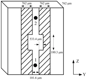
Figure 1. The geometry and dimensions of a coplanar stripline structure.
Figure 2. Comparison of time-domain wave-forms for voltages at observation point 1.
Figure 3. Comparison of time-domain wave-forms for voltages at observation point 2.
Figure 2 and Figure 3 graph the time-domain voltage waveforms at the observation points 1 and 2. It is clear that the proposed formalism is more accurate, and lager errors occur for the ADI-FDTD method. Additionally, S-parameters between the two observation points are calculated, as shown in Figure 4. The result obtained using the proposed method is compared with those of the conventional FDTD and good agreement is observed. The comparison of the numerical performance versus the iteration number is shown in Table 1. The computation time for the ADI-FDTD method is 69 s, while the proposed formalism used 30 s without iteration. With the increase of the iteration number, the CPU time is increased.
The second example is related to the microstrip T-junction of [29], as shown in Figure 5. The substrate is 254-µm-thick and has a relative dielectric constant of 9.9. The microstrip is 230-µm-wide and is assumed to have zero thickness. The microstrip stub is 510-µm-wide and 1380-µm-long. The cell size is chosen to be dx = 63.5µm, dy = 57.5µm, and dz = 102µm. A baseband Gaussian pulse e−((t−tc)/τ)2 with τ = 15 ps andTc = 3τ is used as the excitation to obtain the S-parameters between DC and the 30-GHz band. The Mur’s first-order absorbing boundary condition [26] is implemented to terminate the outer surfaces except for the ground plane on the bottom side. For the conventional FDTD, we choose the time step ΔtFDTD = 0.2 ps. For the ADI-FDTD method, the time step is
ΔtADI= 10 ΔtFDTD. In the Laguerre-based FDTD method, we choose q = 60,s= 1.2×10¹² [27, 28],
Table 1. Simulation results for a coplanar stripline structure.
Scheme Δt Marching-on steps CPU time (s)
FDTD 0.15 ps 3000 98
ADI-FDTD 1.5 ps 300 69
Laguerre-based FDTD
(without iteration) - 81 30
Laguerre-based FDTD
(with one iteration) - 81 54
Laguerre-based FDTD
(with two iterations) - 81 78
Figure 4. Comparison of theS-parameters. Figure 5. The geometry and dimensions of the microstrip T-junction.
Figure 6. Comparison of time-domain wave-forms for voltages at observation point 1.
Figure 8. Comparison of theS-parameters.
Table 2. Simulation results for the microstrip T-junction.
Scheme Δt Marching-on
steps CPU time (s)
Resonant frequency (GHz)
FDTD 0.2 ps 4000 63 1.686
ADI-FDTD 2 ps 400 40 1.541
Laguerre-based FDTD
(without iteration) - 61 9 1.637
Laguerre-based FDTD
(with one iteration) - 61 17 1.656
Laguerre-based FDTD
(with two iterations) - 61 25 1.663
Figure 6 and Figure 7 plot the time-domain voltage waveforms at the observation points 1 and 2. The S-parameters between the two observation points are also extracted from the time-domain data, as shown in Figure 8. It can be seen that the agreement between the conventional FDTD and the Laguerre-based FDTD method is very good. However, the ADI-FDTD method shows large errors when the time step is ten times larger than that used in the conventional FDTD.
The comparison of the computational efficiency and accuracy versus the iteration number is shown in Table 2, the resonant frequency is also considered. It can be see that, with the increase of the numbers of iterations, the accuracy can be improved at the cost of additional CPU time. With two additional iterations, the Laguerre-based method not only achieves about 1.6 times the saving in CPU time in comparison with the ADI-FDTD method but also gives better results than the ADI-FDTD method. In addition, we can see that the simulation takes 63 s for the FDTD method, and 25 s for the proposed method with two additional iterations. The CPU time for the proposed method is reduced to about 39.7% of the FDTD method.
4. CONCLUSION
An efficient Laguerre-based FDTD method is used in this work for the analysis of the planar circuits. The accuracy of the proposed method is improved by using an iterative procedure. To verify the validity of the proposed method, two examples are included. The accuracy of the proposed method has been proved from the comparison of both time domain and frequency domain results. It is demonstrated that the Laguerre-based FDTD method is highly efficient while timesaving compared with the ADI-FDTD method.
ACKNOWLEDGMENT
This work was supported by the National Natural Science Foundation of China under Grant Nos. 41105013, 41375028, and 51277182.
REFERENCES
1. Xu, K., Z. Fan, D.-Z. Ding, and R.-S. Chen, “GPU accelerated unconditionally stable Crank-Nicolson FDTD method for the analysis of three-dimensional microwave circuits,” Progress In Electromagnetics Research, Vol. 102, 381–395, 2010.
2. Mao, Y.-F., B. Chen, H.-Q. Liu, J.-L. Xia, and J.-Z. Tang, “A hybrid implicit-explicit spectral FDTD scheme for the oblique incidence programs on periodic structures,” Progress In Electromagnetics Research, Vol. 128, 153–170, 2012.
3. Pergol, M. and W. Zieniutycz, “Rectangular microstrip resonator illuminated by normal-incident plane wave,” Progress In Electromagnetics Research, Vol. 120, 83–97, 2011.
4. Cao, D.-A. and Q.-X. Chu, “FDTD analysis of chiral discontinuities in waveguides,” Progress In Electromagnetics Research Letters, Vol. 20, 19–26, 2011.
5. Sirenko, K., “An FFT-accelerated FDTD scheme with exact absorbing conditions for characterizing axially symmetric resonant structures,”Progress In Electromagnetics Research, Vol. 111, 331–364, 2011.
6. Kantartzis, N. V., “Hybrid unconditionally stable high-order nonstandard schemes with optimal error-controllable spectral resolution for complex microwave problems,” Int. J. Numer. Model.: Electronic Networks, Devices and Fields, Vol. 25, Nos. 5–6, 621–644, 2012.
7. Kantartzis, N. V., D. L. Sounas, C. S. Antonopoulos, and T. D. Tsiboukis, “A wideband ADI-FDTD algorithm for the design of double negative metamaterial-based waveguides and antenna structures,”IEEE Trans. Magn., Vol. 43, No. 4, 1329–1332, Apr. 2007.
8. Zheng, H., L. Feng, and Q. Wu, “3-D nonorthogonal ADI-FDTD algorithm for the full-wave analysis of microwave circuit devices,”IEEE Trans. Microw. Theory Tech., Vol. 58, No. 1, 128–135, Jan. 2010.
9. Taflove, A., Computational Electrodynamics: The Finite-difference Time-domain Method, Artech House, Norwood, MA, 1995.
10. Chung, Y. S., T. K. Sarkar, B. H. Jung, and M. Salazar-Palma, “An unconditionally stable scheme for the finite-difference time-domain method,”IEEE Trans. Microw. Theory Tech., Vol. 51, No. 3, 697–704, Mar. 2003.
11. Srikumar, S. and A. Gasiewski, “Transient analysis of dispersive, periodic structures for oblique plane wave incidence using Laguerre marching-on-in-degree (MoD),” IEEE Trans. Antennas Propag., Vol. 61, No. 8, 4132–4138, Aug. 2013.
12. He, G., W. Shao, X. Wang, and B. Wang, “An efficient domain decomposition Laguerre-FDTD method for two-dimensional scattering problems,”IEEE Trans. Antennas Propag., Vol. 61, No. 5, 2639–2645, May 2013.
14. Jung, B. H., Z. Mei, and T. K. Sarkar, “Transient wave propagation in a general dispersive media using the Laguerre functions in a marching-on-in-degree (MOD) methodology,” Progress In Electromagnetics Research, Vol. 118, 135–149, 2011.
15. Duan, Y. T., B. Chen, and Y. Yi, “Efficient implementation for the unconditionally stable 2-D WLP-FDTD method,”IEEE Microw. Wireless Compon. Lett., Vol. 19, No. 11, 677–679, Nov. 2009. 16. Duan, Y. T., B. Chen, D. G. Fang, and B. H. Zhou, “Efficient implementation for 3-D Laguerre-based finite-difference time-domain method,” IEEE Trans. Microw. Theory Tech., Vol. 59, No. 1, 56–64, Jan. 2011.
17. Jung, K. Y., F. Teixeira, S. Garcia, and R. Lee, “On numerical artifacts of the complex envelope ADI-FDTD method,”IEEE Trans. Antennas Propag., Vol. 57, No. 2, 491–498, Feb. 2009.
18. Zhang, Y., S. Lu, and J. Zhang, “Reduction of numerical dispersion of 3-D higher order ADI-FDTD method with artificial anisotropy,”IEEE Trans. Microw. Theory Tech., Vol. 57, No. 10, 2416–2428, Oct. 2009.
19. Zheng, H. and K. Leung, “A nonorthogonal ADI-FDTD algorithm for solving 2-D scattering problems,” IEEE Trans. Antennas Propag., Vol. 57, No. 12, 3981–3902, Dec. 2009.
20. Tan, E. and D. Heh, “ADI-FDTD method with fourth order accuracy in time,” IEEE Microw. Wireless Compon. Lett., Vol. 18, No. 5, 296–298, May 2008.
21. Wang, S., F. L. Teixeira, and J. Chen, “An iterative ADI-FDTD with reduced splitting error,”
IEEE Microw. Wireless Compon. Lett., Vol. 15, No. 2, 92–94, Feb. 2005.
22. Wang, S. and J. Chen, “Pre-iterative ADI-FDTD method for conductive medium,” IEEE Trans. Microw. Theory Tech., Vol. 53, No. 6, 1913–1918, Jun. 2005.
23. Welfert, B. D., “Analysis of iterated ADI-FDTD schemes for Maxwell curl equations,”
J. Comput. Phys., Vol. 222, 9–27, Mar. 2007.
24. Jung, K. Y. and F. L. Teixeira, “An iterative unconditionally stable LOD-FDTD method,” IEEE Microw. Wireless Compon. Lett., Vol. 18, No. 2, 76–78, Feb. 2008.
25. Yang, Y., R. S. Chen, W. C. Tang, K. Sha, and K. N. Yung, “Analysis of planar circuits using an unconditionally stable 3-D ADI-FDTD method,” Microwave and Optical Technology Letters, Vol. 46, No. 2, 175–179, Jul. 2005.
26. Mur, G., “Absorbing boundary conditions for the finite-difference approximation of the time-domain electromagnetic field equations,”IEEE Trans. Electromagn. Compat., Vol. 23, No. 4, 377– 382, Nov. 1981.
27. Yuan, M., J. Koh, T. K. Sarkar, W. Lee, and M. Salazar-Palma, “A comparison of performance of three orthogonal polynomials in extraction of wide-band response using early time and low frequency data,”IEEE Trans. Antennas Propag., Vol. 53, No. 2, 785–792, Feb. 2005.
28. Yuan, M., A. De, T. K. Sarkar, J. Koh, and B. H. Jung, “Conditions for generation of stable and accurate hybrid TD-FD MoM solutions,” IEEE Trans. Microw. Theory Tech., Vol. 54, No. 6, 2552–2563, Jun. 2006.