An Analysis of Near-field Scattering Characteristics of Rough
Target: From the Perspective of Bidirectional Reflectance
Distribution Function Based on LS-SVM
Ning Li, Min Zhang*, Ding Nie, and Wangqiang Jiang
Abstract—The near-field scattering characteristics of rough target are analyzed by using a revised bidirectional reflectance distribution function (BRDF) of a rough surface based on least squares support vector machine (LS-SVM). The revised BRDF is more reliable in a larger range of incident angles and scattering angles that beyond the scope of experimental measurements. The basic principle of LS-SVM and the modeling process are firstly introduced in detail. Then the comparison among LS-SVM, the back propagation neural network (BPNN) and the measured data is carried out. The results show that the LS-SVM model has better integrative performance, stronger generalization ability and higher precision. On this basis, the calculation of the near-field radar cross section (RCS) of a complex target is safely performed and analyzed. The method proposed is helpful to better investigate the near-field scattering characteristics of rough target.
1. INTRODUCTION
Generally speaking, it is difficult to calculate the near-field scattering characteristics of rough surfaces. But the bidirectional reflectance distribution function (BRDF) can reflect the optical scattering properties of rough surfaces. It is a critical means to studying the complex laser and infrared light scattering properties. Based on the direct functional relationship between BRDF and the laser radar cross section (LRCS) per unit area, BRDF has been receiving great attention for its myriad applications in research areas such as target detection and recognition, stealth technology and so on [1, 2]. If the reliable BRDF can be obtained in various angle configurations, it will be applied to analyzing the near-field scattering characteristics. Thus, how to get the reliable BRDF will be the primary issue that should be solved.
There are two primary approaches to studying the BRDF, namely, theoretical calculation [3] and experimental measurement [4, 5]. The former needs to obtain the roughness statistical parameters of rough surfaces, and then carry out calculations based on light scattering theory of rough surfaces. Due to the complexity of theoretical calculations and the difficulty to directly obtain the roughness parameters of various materials, experimental measurement is more frequently used in engineering applications. In the laboratory bright sources of light are used to measure the BRDF of sample surfaces, and laser beams are used as sources because of their high brightness, convenience, and availability. But an experiment can be carried out only in a limited range of incident angles and scattering angles, thus, the BRDF model is developed by using the experimental data of different materials to acquire the corresponding BRDF values of the incident angles and scattering angles that can not be easily measured in actual experiment.
There are various ways to establish a BRDF calculation model, such as the geometrical optics theory-based Cook-Torrance model [6], the modified Phong model [7], the Ward model [8] and the Oren-Nayar model [9]. However, most of them are for irregular surfaces which are difficult to be simulated.
Received 8 May 2014, Accepted 14 September 2014, Scheduled 23 September 2014
* Corresponding author: Min Zhang ([email protected]).
Recently, in view of the automation of the fitting function’s selection, two methods have been proposed: artificial neural network (ANN) [10] and support vector machine (SVM) [11]. ANN is for large-sampled data and SVM for small-sampled data. They use kernel function to solve various problems, avoiding selecting the fitting function, which enables the method to be more versatile. However, as a new machine learning approach for small-sampled data developed based on statistics theory, SVM has many unique advantages over ANN in some engineering fields [12].
Using the structural risk minimization principle instead of the empirical risk minimization principle, SVM has the advantages of simple structure, global optimization and strong generalization ability, which makes it a hot spot of the machine learning research. However, the major drawback of SVM is its high computational burden and low training efficiency because of the required constrained optimization programming. With regard to this problem, a new method to establish the BRDF model by Least Squares Support Vector Machine (LS-SVM) is proposed in this paper. While keeping the main merits of standard SVM, LS-SVM has the advantages of simple calculation, high calculation speed and little memory requirement [13], which has a great potential for future application in the calculation of target scattering properties.
The paper is organized as follows. The principle of LS-SVM is mainly introduced in Section 2. On this basis, Section 3 presents the establishment of BRDF model for arbitrary incident angles and scattering angles by appropriately choosing the kernel function and model parameters. The simulated results are shown and analyzed successively in Section 4. Then, the near-field scattering properties of complex target are calculated based on BRDF, and the results are provided in Section 5. Section 6 concludes this paper.
2. THE PRINCIPLE OF LS-SVM
The LS-SVM [14, 15] is a new type of SVM proposed by J. A. K. Suykens in 1999, which can be seen as a development and improvement of standard SVM. The LS-SVM converts the inequality constraints of standard SVM into equality ones, which leads to solving a linear system instead of a quadratic programming problem. Moreover, the number of the unknown parameters of the LS-SVM model built with Radical Basis Function (RBF) is only two, less than those of standard SVM, which greatly simplifies the problem. As a result, the convergence performance is obviously enhanced and the solving process is greatly accelerated. Thus the algorithm is described in detail as follows [16].
Considering a scattered dataset of N points {xk, yk}kN=1, with n-dimensional input data xk ∈Rn
and output data yk∈R, we can define linear equation of higher dimensional feature space:
y=ϕ(x)ωT +b (1)
where the nonlinear mapping ϕ(·): Rn → Rnk maps the input data into a so-called high-dimensional
feature space (which can be infinite-dimensional),ω∈Rnk is weighed value vector andb∈Ris threshold
value. Consequently, the problem of fitting pluralistic nonlinear model can be transformed into linear regressive problem. The optimization problem is replaced by the following equations [17]:
⎧ ⎪ ⎨ ⎪ ⎩
min
ω,b,eJ(ω, e) =
1
2ω
Tω+1
2γ
N
k=1 e2
k
s.t. yk=ωTϕ(xk) +b+ek, k = 1,2, . . . , N
(2)
where the first term stands for the minimization of the Vapnik Chervonenkis (VC) dimension, while the
second one minimizes the training errors (ek). The regularization constantγ >0 is included to control
the bias-variance trade-off.
Note that in some cases,ω becomes infinite dimension, and the above formulation cannot be used
to solve the problem. Therefore, we need to perform the computations in another space, called the dual space of Lagrangian multipliers after applying Mercer’s theorem [18]. Consider the Lagrangian of Eq. (2) given by:
L=J(ω, e)−
N
k=1
Here α= (α1, α2, . . . , αl), αi ∈R are Lagrangian multipliers. By Karush-Kuhn-Tucker (KKT) optimal
conditions [19], the first order conditions for optimality are given by:
⎧ ⎪ ⎪ ⎪ ⎪ ⎪ ⎪ ⎪ ⎪ ⎪ ⎪ ⎪ ⎪ ⎨ ⎪ ⎪ ⎪ ⎪ ⎪ ⎪ ⎪ ⎪ ⎪ ⎪ ⎪ ⎪ ⎩ ∂L
∂ω = 0→ω =
N
k=1
αkϕ(xk)
∂L
∂b = 0→
N
k=1
αk= 0
∂L
∂ek = 0→αk=γek
∂L
∂αk = 0→ω Tϕ(x
k) +b+ek−yk= 0
k= 1,2, . . . , N (4)
Eq. (4) can be written successively as the solution to the following set of linear equations
⎡ ⎢ ⎣
I 0 0 −ϕ(xn)
0 0 0 −1n
0 0 γI −I
ϕ(xn)T 1n I 0
⎤ ⎥ ⎦ ⎡ ⎢ ⎣ ω b e α ⎤ ⎥ ⎦= ⎡ ⎢ ⎣ 0 0 0 y ⎤ ⎥ ⎦ (5)
After eliminating ω,efrom the equations, combining with Mercer conditions K(xk, xl) =ϕ(xk)Tϕ(xl),
we obtain:
0 1Tn
1n Ω +γ−1I
b α = 0 y (6)
where y = [y1, . . . , yN]T, 1n = [1, . . . ,1]T,α = [α1, . . . , αN]T, Ω = K(xk, xl), k, l = 1,2, . . . , N, I is an
identity matrix. From Eq. (6), the regression parametersb and α can be solved as
b = 1
T
n(Ω +γ−1In)−1y 1Tn(Ω +γ−1I
n)−11n (7)
α = Ω +γ−1In−1(y−1nb) (8)
Thus, the regression function is expressed in dual form as
y(x) =
N
k=1
αkK(xk, x) +b (9)
3. THE ESTABLISHMENT OF BRDF MODEL
Given a training data set{xk, yk}Nk=1, herexk ∈Rn aren influencing factors of the BRDF values and
yk∈R are measured values of BRDF, the modeling procedure is expressed as follows.
(a) Divide the samples into two parts: the training data that is used to build up the model and the test data that is used to test the model generalization capability.
(b) Select appropriate kernel function and parameters and train the samples with the LS-SVM
regression algorithm. Calculate the support vector α and the corresponding threshold b using
Eq. (7) and Eq. (8), then establish the LS-SVM data processing model.
3.1. The Choice of Kernel Function
Kernel function is the core of SVM. The choice of kernel function will greatly influence the learning ability and generalization ability of machine learning. Different kernels determine different nonlinear transformations and characteristics spaces, thus selecting different kernels to train SVM will lead to
different results. Any functionK(xi, xj) satisfying Mercer’s condition can be used as the kernel function.
Thus different kernel functions possess their respective traits, and exert varying degrees of influences on recurrent LS-SVM performance. Among these functions, the RBF function can map the sample set from the input space into a high-dimensional feature space effectively, which is helpful for representing the complex nonlinear relationship between the output and input samples. Based on this, the RBF function is used widely. In this paper, RBF function is also selected as the kernel function, which is expressed as follows:
K(xi, xj) =e−||xi−xj||2/σ2 (10)
3.2. The Choice of the Model Parameters
As a very important part in LS-SVM modeling, the choice of parameters directly affects the accuracy of data fitting, generalization ability as well as the training speed. For a specific problem, inappropriate parameters may lead to unexpected results of data fitting and forecasting.
Due to the selection of RBF as the kernel function, it can be seen that there are two free parameters,
regularization parameterγ and kernel width parameterσ, that have to be properly optimized. The first
parameterγdetermines the trade-offs between the minimization of the fitting error and the minimization
of the model complexity. For the definite dataset, a small value of γ denotes a slight penalty on the
experience error, a low complexity of the learning machine and a high experience risk, which is called
“under-fitting”. The bigger of the γ value, the longer the training time will be. But too big a value
of γ will cause over-fitting and decline of the generalization ability. The second parameter σ mainly
affects the complexity of the distribution of samples in high-dimensional feature space. The fitting
error will decrease as the value ofσ gets small, but too small a value ofσ could also cause over-fitting.
In order to obtain a pair of superior parameters, we have to change the parameters and carry on the training for many times. Finally the parameters of the learning machine are acquired according to all the previous test results. There could be several parameter selection methods such as cross-validation type method [20], leave-one-out method, grid-search method and three-step-search method [21]. In this paper we use the three-step-search method.
4. MODELING RESULTS AND ANALYSIS
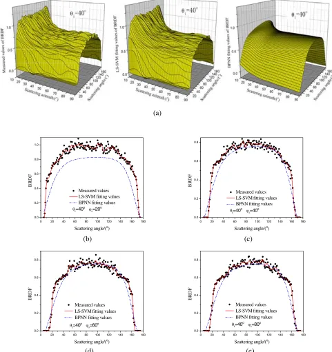
The material used for modeling and testing in this paper is a kind of paint and the wavelength of the
incident light is 0.905µm. Here, the measured data of BRDF has four influencing factors (θi, ϕi, θs, ϕs),
these four angles are respectively denoted as incident angle, incident azimuth, scattering angle and
scattering azimuth. The sample data are obtained within the following angle range: θi ∈ [30◦,90◦]
with a sampling interval of 5◦, ϕi is fixed to 20◦, θs ∈ [5◦,175◦] with a sampling interval of 1◦ and
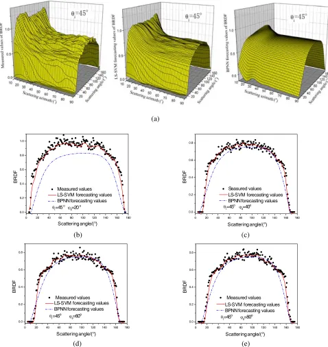
ϕs ∈ [10◦,90◦] with a sampling interval of 10◦. The above data are divided into two categories: test
sample data and training sample data, and the test sample data are chosen in the angle range ofθi = 45◦
and 75◦,ϕi = 20◦,θs∈[5◦,90◦] and ϕs∈[10◦,90◦].
After several adjustments, the optimal values of γ and σ2 are 1513.0 and 48.0 respectively for
the LS-SVM model and the following calculation results shown in Fig. 1 and Fig. 2. Moreover, the back propagation neural network (BPNN) [22] fitting data are also provided to be compared with those obtained by LS-SVM in Fig. 1 and Fig. 2. BPNN is a popular neural network algorithm with wide applications, which has the main advantage that it can minimize the error sum of square between the actual data and the desired data. The root mean square error (RMSE) is used to evaluate the effect.
ERMSE=
N
i=1
yi−y
i2
(a)
0 20 40 60 80 100 120 140 160 180 0.0
0.2 0.4 0.6 0.8 1.0
Measured values LS-SVM fitting values BPNN fitting values
θi=40o
ϕs=20o
BRD
F
Scattering angle/(o
)
0 20 40 60 80 100 120 140 160 180 0.0
0.2 0.4 0.6 0.8
Measured values LS-SVM fitting values BPNN fitting values
θi=40
o
ϕs=40
o
BRD
F
Scattering angle/(o
)
(b) (c)
0 20 40 60 80 100 120 140 160 180 0.0
0.2 0.4 0.6 0.8
Measured values LS-SVM fitting values BPNN fitting values
BRD
F
Scattering angle/(o
)
0 20 40 60 80 100 120 140 160 180 0.0
0.2 0.4 0.6 0.8
Measured values LS-SVM fitting values BPNN fitting values
BRD
F
Scattering angle/(o
)
(d) (e)
θi=40
o
ϕs=60
o θ
i=40
o
ϕs=80
o
Figure 1. Comparison between measured values and fitting values with θi = 40◦ (The values of θi participate in the training). (a) 3D distribution of the measured BRDF data, LS-SVM fitting BRDF
data and BPNN fitting BRDF data (from left to right). (b) ϕs = 20◦. (c) ϕs = 40◦. (d) ϕs = 60◦.
(e)ϕs= 80◦.
N is the number of the sample, yi the forecasting data of each sample, andyi the measured value.
From the comparisons shown in Fig. 1 and Fig. 2, we can see that both the LS-SVM model’s fitting data and forecasting data agree with the measured data with smaller errors and higher precision.
(a)
0 20 40 60 80 100 120 140 160 180 0.0
0.2 0.4 0.6 0.8 1.0
Measured values LS-SVM forecasting values BPNN forecasting values
θi=45
o
ϕs=20
o
BRD
F
0 20 40 60 80 100 120 140 160 180 0.0
0.2 0.4 0.6 0.8
Seasured values
θi=45
o
ϕs=40
o
BRD
F
(b) (c)
0 20 40 60 80 100 120 140 160 180 0.0
0.2 0.4 0.6 0.8
Measured values
θi=45
o ϕ s=60
o
BRD
F
0 20 40 60 80 100 120 140 160 180 0.0
0.2 0.4 0.6 0.8
Measured values
θi=45
o ϕ s=80
o
BRD
F
Scattering angle/(o )
(d) (e)
LS-SVM forecasting values BPNN forecasting values
LS-SVM forecasting values
BPNN forecasting values LS-SVM forecasting valuesBPNN forecasting values Scattering angle/(o
) Scattering angle/(o
)
Scattering angle/(o)
Figure 2. Comparison between measured values and forecasting values withθi = 45◦.(The values ofθi don’t participate in the training). (a) 3D distribution of the measured BRDF data, LS-SVM forecasting
BRDF data and BPNN forecasting BRDF data (from left to right). (b) ϕs = 20◦. (c) ϕs = 40◦.
(d)ϕs= 60◦. (e)ϕs= 80◦.
z
x
y
s
γ
Δ
Δ
γ
is
γ
O
i
γ
h
(a)
(b)
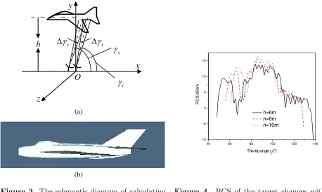
Figure 3. The schematic diagram of calculating scattering characteristics of the target.
40 60 80 100 120 140 -10
-5 0 5 10 15
h=6m
h=8m
h=10m
RCS/dBsm
The dip angle γi/(o
)
Figure 4. RCS of the target changes with the
dip angle γi.
5. THE APPLICATION OF LS-SVM IN CALCULATING NEAR-FIELD SCATTERING CHARACTERISTICS OF COMPLEX TARGET
Figure 3(a) shows the schematic diagram of calculating the near-field scattering characteristics of the target. The whole target relative to the emitter is in the near-field region. The laser only illuminates a small portion of the target at a time, and the surface of effective irradiated area can be dissected into small triangle facets. These facets can be characterized by their node coordinates, area sizes and normal vectors. Each surface facet relative to the emitter is in the far-field region and can be studied by using far-field method [23]. The echo power of each facet can be expressed as
ΔPs= PiΔsσ
0
4πcosθiRliml→∞ Ar
R2
l
(12)
where Pi is the power of each facet intercepted, Δsthe area of each facet, σ0 the average value of the
RCS per unit area, θi the incident angle, Rl the range between the detector and the facet, andAr the
aperture area of the detector.
In the other formulation entailing the BRDF, the echo power is
ΔPs =frPiΔscosθs lim
Rl→∞ Ar
R2
l
(13)
fr is the BRDF at incident angle θi and scattering angle θs. By comparing Eq. (12) and Eq. (13), we
get
σ0 = 4πf
rcosθicosθs (14)
Combining Eq. (14) and the effective irradiation area, the RCS of the whole target can be obtained.
In this paper, we use the Gaussian-beam wave model [24] for calculation. h denotes the distance
from the detector to the target, the width of the transmitting beam (denoted by Δγi) is 3◦ and the
angle between the beam andx-axis is denoted byγi. The distance that from the detector to the emitter
is 0.03 m. The width of the receiving beam (denoted by Δγs) is also 3◦, and the angle between it and
of about 12.5 m, a height of about 3 m and a width of about 9 m, as is illustrated in Fig. 3(b), assuming the surface of the plane is coated with the paint that used in the experiment in Section 4.
Here, the site of the target is fixed. The angle ofγichanges gradually from 0◦ to 180◦, and the angle
ofγsis always two degrees larger thanγi. The variation of RCSs with the dip angleγi is simulated and
shown in Fig. 4, in which the emitter is supposed to be 10 m, 8 m and 6 m below the target respectively. The results show that the RCS peaks appear on the wings and the empennages. This may be due to the fact that the irradiation area is larger in these two parts. Moreover, the value of the peaks rises
with the increase of heighth.
6. CONCLUSIONS
This paper presents a new attempt to evaluate the laser scattering properties of complex targets in the near-field region based on the revised BRDF model of rough surface materials. It is worth noting that the revised BRDF model is reliable in a relatively larger range of incident angles and scattering angles by using the LS-SVM. The comparison of the measured data and the forecasting values just verifies the LS-SVM model. On this basis, the calculation of the near-field RCS of a complex target is safely performed and analyzed. Although the calculation of RCS presented in this work is only limited to a plane-like target, the outline and corresponding conclusions will help to better investigate the near-field scattering characteristics of rough targets from the perspective of BRDF. Future work will be carried out to study the near-field scattering characteristics of much more complex targets by using the revised BRDF based on LS-SVM.
ACKNOWLEDGMENT
The authors would like to thank the Fundamental Research Funds for the Central Universities and the National Natural Science Foundation of China under Grant Nos. 41306188 and 61372004 to support this kind of research.
REFERENCES
1. Gibbs, D. P., C. L. Betty, A. K. Fung, and A. J. Blanchard, “Automated measurement of polarized
bidirectional reflectance,” Remote Sensing of Environment, Vol. 43, 97–114, 1993.
2. Li, H. K., N. Pinel, and C. Bourlier, “A monostatic illumination function with surface reflections
from one-dimensional rough surfaces,” Waves in Random and Complex Media, Vol. 21, 105–134,
2011.
3. Ulaby, F. T., R. K. Moore, and A. K. Fung, Microwave Remote Sensing, Addison-Wesley, New
York, 1982.
4. Arai, K., “Method for estimation of grow index of tealeaves based on Bi-directional reflectance
distribution function: BRDF measurements with ground based network cameras,” International
Journal of Applied Sciences, Vol. 2, 52–62, 2011.
5. Jordan, D. L., “Experimental measurements of optical backscattering from surfaces of roughness
comparable to the wavelength and their application to radar sea scattering,” Waves in Random
and Complex Media, Vol. 5, 41–54, 1995.
6. Cook, R. L. and K. E. Torrance, “A reflectance model for computer graphics,”Computer Graphics,
Vol. 15, 307–316, 1981.
7. Phong, B. T., “Illumination for computer generated pictures,” Communications of the ACM,
Vol. 18, 311–317, 1975.
8. Ward, G. J., “Measuring and modeling anisotropic reflection,” Computer Graphics, Vol. 26, 265–
272, 1992.
9. Oren, M. and S. K. Nayar, “Generalization of the Lambertian model and implications for machine
10. Li, W., J. F. Chen, and T. Wang, “Prediction of the plasma distribution using an artificial neural
network,” Chinese Physics B, Vol. 18, 2441–2444, 2009.
11. Vapnik, V., E. Levin, and Y. Le Cun, “Meaning the VC-dimension of a learning machine,”Neural
Computation, Vol. 6, 851–876, 1994.
12. Balabin, R. M. and E. I. Lomakina, “Support vector machine regression (SVR/LS-SVM)-an alternative to neural networks (ANN) for analytical chemistry? Comparison of nonlinear methods
on near infrared,”Analyst, Vol. 136, 1703–1712, 2011.
13. Wang, H. F. and D. J. Hu, “Comparison of SVM and LS-SVM for regression,” International
Conference on Neural Networks and Brain, Vol. 1, 279–283, 2005.
14. Suykens, J. A. K. and J. Vandewaiie, “Least squares support vector machine classifiers,” Neural
Processing Letter, Vol. 9, 293–300, 1999.
15. Suykens, J. A. K., T. V. Gestel, J. D. Brabanter, B. D. Moor, and J. Vandewalle, Least Squares
Support Vector Machines, World Scientific Publishers, Singapore, 2002.
16. Adankon, M. M., M. Cheriet, and A. Biem, “Semisupervised learning using Bayesian interpretation:
Application to LS-SVM,” IEEE Transactions on Neural Networks, Vol. 22, 513–524, 2011.
17. Gestel, V., et al., “Financial time series prediction using least squares support vector machines
within the evidence framework,”IEEE Transactions on Neural Networks, Vol. 12, 809–821, 2001.
18. Scholkopf, B. and S. Mika, “Input space vs. feature space in Kernel based methods,”IEEE Trans.
on Neural Networks, Vol. 10, 1000–1017, 1999.
19. Fletcher, R., Practical Methods of Optimization,John Wiley and Sons, Chichester and New York,
1987.
20. Browne, M. W., “Cross-validation methods,” Journal of Mathematical Psychology, Vol. 44, 108–
132, 2000.
21. Guo, H., H. P. Liu, and L. Wang, “Method for selecting parameters of least squares support vector
machines and application,” Journal of System Simulation, Vol. 18, 2033–2036, 2006.
22. Hecht-Nielsen, R., “Theory of the backpropagation neural network,”International Joint Conference
on IEEE, 93–605, 1989.
23. Tomiyasu, K., “Relationship between and measurement of differential scattering coefficient and
bidirectional reflectance distribution function (BRDF),” IEEE Transactions on Geoscience and
Remote Sensing, Vol. 26, 660–665, 1988.
24. Andrews, L. C., M. A. Al-Habash, C. Y. Hopen, and R. L. Phillips, “Theory of optical scintillation: