© 2015, IJCSMC All Rights Reserved
112
International Journal of Computer Science and Mobile Computing
A Monthly Journal of Computer Science and Information Technology
ISSN 2320–088X
IJCSMC, Vol. 4, Issue. 1, January 2015, pg.112 – 119
RESEARCH ARTICLE
IMAGE COMPRESSION USING HIRARCHICAL
LINEAR POLYNOMIAL CODING
Rasha Al-Tamimi
1, Ghadah Al-Khafaji
21,2
Dept. of Computer Science, College of Science, University of Baghdad, Baghdad, Iraq
1[email protected]
;
2[email protected]
Abstract—In this paper a hierarchal modelling based is introduced for compressing images, it is based utilizing the layered representation along with the polynomial coding. The test results showed best performance of the hierarchal polynomial coding compared to the traditional polynomial coding.
Keywords— image compression, redundancy, modeling, hierarchal scheme, polynomial coding
I. INTRODUCTION
In recent years, a dramatic increase in the amount of information available in the form of digital image data, it become necessary to solve the problems of storage and time issues by utilizing image compression of redundancy removal based. In general, Image compression techniques generally fall into two categories: lossless and lossy depending on the redundancy type exploited, where lossless also called information preserving or error free techniques, in which the image compressed without losing information that rearrange or reorder the image content, and are based on the utilization of statistical redundancy alone such as Huffman coding, Arithmetic coding and Lempel-Ziv algorithm, while lossy which remove content from the image, which degrades the compressed image quality, and are based on the utilization of psycho-visual redundancy, either solely or combined with statistical redundancy such as vector quantization, fractal, block truncation coding and JPEG [1], reviews of lossless and lossy techniques can be found in [2],[3],[4]-[7]. Modelling or a Mathematical Model is a simple description formula utilized efficiently in image compression problem to remove the correlation embedded between image pixel neighbours (spatial/interpixel redundancy). A compression system of modelled based, is generally composed of two parts; one corresponds to mathematical function (deterministic part) exploited to create an approximation modelled image that resemble the original image, and the second part corresponds to the error or residual (probabilistic part) as a difference between original and the approximated. For more details see [8], [9], [10]. Polynomial coding is modelling based technique exploited by a number of researchers as a tool to compress images [11], [12], [13]-[16]. The techniques characterized by simplicity of implementation, efficiency in reducing image information into small effective coefficients.
© 2015, IJCSMC All Rights Reserved
113
II. THEPROPOSEDCOMPRESSIONSYSTEM
The main taken concerns in the proposed system are:
1- Polynomial coding of linear approximation model is exploited to compress image efficiently using the three coefficients (a0,a1 and a2) representation that remove the redundancy between the image itself. 2- The top-down layered or hierarchal scheme is adopted to remove the redundancy embedded within the coefficients to improve the compression ratio with preserving image quality.
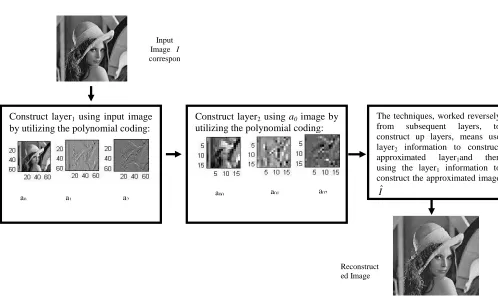
The steps below illustrated the system implantation in more details; Figure (1) shows the basic steps clearly:
Step 1: Load the input uncompressed image I of size N×N that corresponds to layer0 or the root of the hierarchal
representation.
Step 2: Construct the first layer hierarchal representation corresponds to layer1 using the linear polynomial coding
techniques, such as:
1. Partition the input image I into non-overlapping blocks of fixed sized n×n (i.e., 4×4, 8×8). 2. Find the coefficients of the linear approximation model, using the equations below [17]:
1 0 1 00
(
,
)
...
...(
1
)
1
n i n jj
i
I
n
n
a
) 2 ...( ... ) ( ) ( ) , ( 1 0 1 0 2 1 0 1 0 1
n i n j c n i c n j x j x j j i I a ) 3 ...( ) ( ) ( ) , ( 1 0 1 0 2 1 0 1 0 2
n i n j c n i c n j y i y i j i I aWhere I(i,j) is the original image block of size (n×n) and
) 4 ...( ... ... 2 1 yc n xc
Here the (j-xc) and (i-yc) corresponds to the variables of the polynomial that measure the distance of pixel coordinates to
the block center (xc, yc). The a0 coefficients represent the block mean, the a1 coefficients and a2 coefficients represent
the ratio of sum pixel multiplied by the distance from the center to the squared distance in i and j coordinates respectively.
3. Quantized/dequantized the a1and a2 computed coefficients above, using the uniform scalar quantizer.
) 6 ...( ) ( ) 5 ( ... ) ( 1 1 2 1 2 2 1 1 1 1 1 1 a a a a QS Q a D a QS a round Q a QS Q a D a QS a round Q a
One quantization step QSa1 is adopted for the a1 and a2 coefficients (the same quantization step used for both of
© 2015, IJCSMC All Rights Reserved
114
(layer1 coefficients), the a0 corresponds to mean (average) of the image, the linear polynomial coding techniques
utilized, as follows:
1. Partition the computed a0 from layer1 into non-overlapping blocks of fixed sized n×n (i.e., 4×4, 8×8), the size of a0 is
equal to N/n×N/n .
2. Find the coefficients of a0 of the linear approximation model, using the equations below:
1 0 1 0 000 (, )...(7)
1 n i n j j i a n n a ) 8 ...( ) ( ) ( ) , ( 1 0 1 0 2 1 0 1 0 0 01
n i n j c n i c n j x j x j j i a a ) 9 ...( ) ( ) ( ) , ( 1 0 1 0 2 1 0 1 0 0 02
n i n j c n i c n j y i y i j i a aWhere a0(i,j) is the mean of original image of block of size (n×n) and
) 10 ...( ... ... 2 1 yc n xc
The a00, a01 and a02 coefficients correspond to layer2 constructed using the a0 coefficients from layer1 that regarded as
an image.
3. Quantized/dequantized the a00, a01 and a01computed coefficients above, using the uniform scalar quantizer.
) 13 ...( ) ( ) 12 ( ... ) ( ) 11 ...( ) ( 01 02 02 01 02 02 01 01 01 01 01 01 00 00 00 00 00 00 a a a a a a QS Q a D a QS a round Q a QS Q a D a QS a round Q a QS Q a D a QS a round Q a
Two quantization steps QSa0,QSa1 adopted one for the a00 coefficients, and one for a01 and a02 coefficients, for the
quantizeda00Q,a01Q,a02Q/dequantizeda00D,a01D,a02D coefficients.
4. Determine the deterministic part (function formula) 0a~ of mathematical linear model base using the dequantized coefficient and the variables.
)
14
...(
)...
(
)
(
~
02 01 000
a
D
a
D
j
x
ca
D
i
y
ca
5. Find the probabilistic part or error (residual) as a difference between the modelled approximated image
0
~
a and the original one a0. ) 15 ...( ... ~ 0 0 0E a a
© 2015, IJCSMC All Rights Reserved
115
6. Quantized/dequantized the error, using the uniform scalar quantizer.
) 16 ...( )
( 0 0 0
0 0
0 E E a E
E a
E a D a Q QS
QS a round EQ
a
Where QSa0Eis the error quantization step for the quantized a0EQ/dequantized a0EDcoefficients.
Step 4: Build the approximated up layers from the subsequent layers, namely construct layer1 from layer2 and layer0
from layer1, such as:
1. Build the modeled approximated 0aˆ corresponds to layer1, using the two modeling parts, approximated 0a~
and the error a0ED.
)
17
...(
...
...
~
ˆ
0a
0a
0D
a
E2. Determine the deterministic part I~ of mathematical linear model base using the dequantized coefficient of layer1&layer2, and the variables
)
18
...(
...
)...
(
)
(
0
ˆ
~
2 1
D
j
x
ca
D
i
y
ca
a
I
3. Find the probabilistic part or error (residual) as a difference between the modelled approximated image I~ and the original one I.
)
19
...(
...
~
I
I
IE
4. Quantized/dequantized the error IE, using the uniform scalar quantizer.
) 20 ...( )
( IE
IE
QS IEQ IED QS
IE round
IEQ
Where QSIEis the error quantization step for the quantized IEQ/de-quantized IEDcoefficients.
5. Build the modeled approximatedIˆcorresponds to layer0, using the two modeling parts, approximated I ~
and the errorIED.
)
21
....(
...
...
~
ˆ
I
IED
I
6. Encode the layer2 information of quantized coefficients (a00D,a01D,a02D) and the quantized error (a0ED) along
with the layer0 information of quantized coefficients (a1D,a2D) and the quantized error (IE) using LZW coding
techniques.
The techniques, worked reversely from subsequent layers, to construct up layers, means using the coefficients (a00,a01,a02) of layer2 to construct approximated layer1( 0aˆ ) and then using the layer1 coefficients ( 0aˆ ,a1,a2) to
© 2015, IJCSMC All Rights Reserved
116
Fig. (1): The proposed hierarchal polynomial compression system in practical example.
Experimental Results
Experiments were done to compare the performance of the suggested the hierarchical polynomial coding with the traditional polynomial using a fixed block of size 4×4, with various quantization steps for errors (residual images) in layer1 and layer2, whereas the quantization steps for the coefficients adopted the as the identical for the both layers (i.e., use the same quantization step for the coefficients in layer1 and layer2
a0,a1,a2, a00, a01 and a02 ). All the images used are standards (see Figure 2 for an overview) of 256 gray levels (8bits/pixel) of size 256×256.
The Compression ratio (ratio of original size to the compressed size in byte) and the Peak Signal to Noise
Ratio (PSNR) adopted as an objective fidelity measure between the original image
I
and the decodedimage
I
ˆ
as in equation (22).) 22 ..( ... 1
0 1
01
)] , ( ) , ( ˆ [ 1
255 log
10 2
2 10
N x
N y
y x I y x I N
N PSNR
Construct layer1 using input image by utilizing the polynomial coding:
Input Image I correspon
ds to layer0
The techniques, worked reversely from subsequent layers, to construct up layers, means use layer2 information to construct
approximated layer1and then
using the layer1 information to
construct the approximated image Iˆ
Reconstruct ed Image
a0 a1 a2
Construct layer2 using a0 image by utilizing the polynomial coding:
© 2015, IJCSMC All Rights Reserved
117
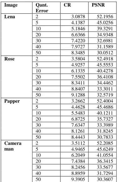
The experimental results are listed in tables (1) and (2) for traditional and hierarchal polynomial coding respectively, that showed that the performance improved using hierarchical polynomial coding techniques in terms of compression ratio about one and a half on average along due to the reduction of a0 resolution (i.e., a0 corresponds to mean of the image implicitly meaning overburden problem that consuming extra large number of bits) with the preserving the image quality.
Generally, two layers construction is sufficient to remove the redundancy, actually there’s no need to extend the work to third layer where’s no correlation embedded between layer2 coefficients.
Lastly, there’s a trade off between compression ratio and the quality affected by the quantization step and the block size, where for high quality image, low compression ratio achieved, that implicitly means small block size utilized with low quantization step, and vice versa, figure(3) shows an example of decoded images.
c a b
a a
Fig. (2): Tested images (a) Lena, (b) Cameraman (c)Rose and (d) Paper, gray scale images of size 256×256.
d c a
Fig. (3): Decoded image using the hierarchal polynomial coding, using quantization coefficients equals to 1 for both layers, quantization step of error layer1 error is equal to 50, with (Case1) quantization step of error layer2 is equal to
2 and (Case2) quantization step of error layer2 is equal to 20 CR=10.1339
PSNR=30.0385
CR= 11.2663 PSNR=30.3454
CR=11.4075 PSNR= 32.5459
CR=10.0055 PSNR= 30.775
Case1
CR= 11.5076 PSNR= 28.9208
CR= 12.6469 PSNR= 29.7171
CR= 13.2825 PSNR= 30.1770
CR= 11.4274 PSNR= 29.3641
© 2015, IJCSMC All Rights Reserved
118
Table 1: Traditional polynomial coding with quantizationstep equal to one for all the coefficients
Table 2: Hierarchal polynomial coding with quantization step equal to one for all the coefficients in layer1&layer2 uses a selected case from the traditional polynomial coding when
quantization of error is equal to 50.
Image Qant.
Error
CR PSNR
Lena 2 3.0878 52.1956
5 4.1387 45.0256
10 5.1846 39.3291
20 6.6366 34.9348
30 7.4220 32.6981
40 7.9727 31.1589
50 8.3485 30.0512
Rose 2 3.5804 52.4918
5 4.9257 45.5553
10 6.1335 40.4278
20 7.5502 36.4108
30 8.3411 34.4462
40 8.8407 33.3011
50 9.1288 32.5719
Papper 2 3.2662 52.4004
5 4.4628 45.4686
10 5.5483 40.1211
20 6.8725 35.7327
30 7.6347 33.3989
40 8.1261 31.8245
50 8.4443 30.7833
Camera man
2 3.5112 52.2085
5 4.9465 45.6249
10 6.2049 41.0554
20 7.4384 36.3415
30 8.2456 33.5677
40 8.8959 31.7294
50 9.3905 30.3607
Image Qant.
Error
CR PSNR
Lena 2 3.0878 52.1956
5 4.1387 45.0256
10 5.1846 39.3291 20 6.6366 34.9348 30 7.4220 32.6981 40 7.9727 31.1589 50 8.3485 30.0512
Rose 2 3.5804 52.4918
5 4.9257 45.5553
10 6.1335 40.4278 20 7.5502 36.4108 30 8.3411 34.4462 40 8.8407 33.3011 50 9.1288 32.5719
Papper 2 3.2662 52.4004
5 4.4628 45.4686
10 5.5483 40.1211 20 6.8725 35.7327 30 7.6347 33.3989 40 8.1261 31.8245 50 8.4443 30.7833
Camera man 2 3.5112 52.2085
5 4.9465 45.6249
© 2015, IJCSMC All Rights Reserved
119
References
[1] Ghadah, Al-K,” Image Compression based on Quadtree and Polynomial. International Journal of Computer Application”s,Vol. 76,No. 3,pp.31-37,2013
[2]Khobragede, P. and Thakare, S. Image Comprssion Techniques-A Review International Journal of Computer Science and Information Technologies, Vol.5,No.1,pp. 272-275,2014.
[3] Marimuthu, M. and Swaminathan, P. Review Article:” An Overview of Image Compression Techniques”. Research Journal of Applied Science, Engineering and Technology, Vol .24,No.4,pp. 5381 -5386,2014
[4]Gonzalez, R. C., “Digital Image Processing", International Society for Optical Engineering (SPIE) ” , 2 Edition, 2002.
[5] Sachin, D.” A Review of Image Compression and Comparison of its Algorithms”. International Journal of Electronics & Communication Technology, Vol.2,No.1,pp22-26 , 2011.
[6] Anitha, S.”2D Image Compression Technique-A Survey”. International Journal of Scientific & Engineering Research, Vol.2,No.7, pp.1 -6,2011
[7] Amruta, S.G. and Sanjay L.N, “A Review on Lossy to Lossless Image Coding”. International Journal of Computer Applications (IJCA),Vol. 67,No.17,pp. 9-16.,2013
[8]Ghadah,Al-K, “Intra and inter frame compression for video streaming”.PhDthesis,Extraunion,UK.2012
[9] Huda, M. “Lossless Image Compression Using Prediction Coding and LZW Scheme. High Diploma Dissertation, Baghdad University.2011
[10] Sinan ,D, “ Medical Image Compression”. High Diploma Dissertation, Baghdad University.2014
[11]George, L. E. and Sultan, B.. “ Image Compression Based on Wavelet, Polynomial and Quadtree”. Journal of Applied Computer Science & Mathematics, Vol.11,No.5,pp. 15-20,2011
[12]George, L. E. and Ghadah, Al-K. “Fast Lossless Compression of Medical Images based on Polynomial”. International Journal of Computer Applications Vo. 70, No.15,pp.0975-8887,2013
[13] Ghadah, Al-K.. “Wavelet Transform and Polynomial Approximation Model for Lossless Medical Image Compression”. International Journal of Advanced Research Computer Science and Software Engineering, Vol.4,No.1 pp.584-587,2014
[14] Haider, Al-M., “Selective Bit Plane Coding and Polynomial Model for Image Compression”, International Journal of Advanced Research in Computer Science and Software Engineering ,Vo.4,No.4 pp. 797-801,2014
[15] Haider, Al-M., and Zainab, Al-R, “.Lossless Image Compression based on Predictive Coding and Bit Plane Slicing”,International Journal of Computer Applications, Vo. 93, p1,2014
[16] Ghada ,Al-K, “ Hierarchical Autoregressive for Image Compression”, Journal of College of Education for Pure Sciences, Vol. 4 No.1,pp 236- 241,2014