Generalized Exponential Matrix Technique Application
for the Evaluation of the Dispersion Characteristics
of a Chiro-Ferrite Shielded Multilayered Microstrip Line
Samiha Daoudi1, Fatiha Benabdelaziz1, Chemseddine Zebiri2, *, and Djamel Sayad3
Abstract—In this work, a new analytical matrix formulation approach for the characterization of a microwave planar structure printed on a complex medium is detailed. The approach is based on the Generalized Exponential Matrix Technique (GEMT) combined with the Method of Moments (MoM)and Galerkin’s procedure. The mathematical calculation development is a robust approach that exclusively uses matrix formulations starting from Maxwell’s equations until the derivation of a compact form of the Green’s tensor of the studied structure. Reduced complexity and calculation simplicity foundation of the applied approach have actually incited the authors to consider the case study of a complex bianisotropic lossy chiral substrate medium. The complexity of the medium is expressed by full tensors form of all four constitutive parameters: permittivity, permeability and magnetoelectric parameters, each is represented by a nine-element tensor. To investigate the electromagnetic behavior of complex media, results of particular bianisotropy cases are presented and discussed. Original results of the biaxial chiral anisotropy case are carried out, discussed and compared with data available in literature.
1. INTRODUCTION
Since the first carried out research works on planar transmission lines in 1952, the microstrip line coplanar line and slot line have become the most known and commonly used planar transmission lines in microwave technology and microwave integrated circuits (MIC) devices [1]. Nowadays, transmission line-based microwave devices are largely used in telecommunication systems to constantly improve the overall performances by reducing the size, weight, and cost [2].
Microstrip lines are used at frequencies from a few megahertz to tens of gigahertz. Their fabrication technology offers at the same time simplicity and facility of realization and integration in microwave devices. Covered microstrips with air gap between the dielectric substrate and the ground plane present less losses than the conventional microstrip lines [3].
The Generalized Exponential Matrix Technique (GEMT) in the spectral domain is a rigorous method used to characterize the interaction of electromagnetic waves with bianisotropic multilayer structures. This technique, proposed by Tsalamengas [4], is used to study source radiations and wave propagation problems in multilayer structures with bianisotropic media [5]. This technique exhibits an elegant and systematic formulation. It has been developed by combining the Fourier transform with the matrix analysis method [6, 7].
In the last few years, the linear complex materials have gained much attention in electromagnetic
applications. Among these materials the bianisotropic media, characterized by four independent
constitutive tensors, are well mentioned. Theoretical research works have known an important progress
Received 21 August 2017, Accepted 25 September 2017, Scheduled 9 October 2017
* Corresponding author: Chemseddine Zebiri ([email protected]).
dealing with their electromagnetic characterization and possibilities of potential applications of complex bianisotropic materials have greatly increased [6–8]. Complex media, such as magnetoelectric (ME) materials [9], have recently attracted much researcher attention. The ME effect [10] in complex materials is known as a product tensor property, which results from the cross interaction between different orderings of the two phases in the composite [10]. The chiral is considered as a complex medium. It is used as substrates and superstrates in the design of printed antennas [11]. The resolution of Maxwell’s equations, in such structures, was not completely finished before 2001 [12]. Since then, the interaction of electromagnetic fields with chiral materials has been studied, in which the chiral medium is used in many applications, microstrip substrates and superstrates [13, 14], and waveguides [15]. The propagation characterization in bianisotropic medium transmission lines have also prompted some interesting works [6, 16].
In this study, we develope a GEMT-based mathematical formulation for a covered suspended bianisotropic substrate microstrip line using the MoM and the Galerkin’s procedure in the spectral
domain. The effect of the medium bianisotropy on the dispersion characteristics is presented
and analyzed. Results are compared with the isotropic case reported in literature showing good
agreements [16, 17].
The novelty of this work lies in a complete matrix formulation of calculation development starting from Maxwell’s equations until the derivation of the Green tensor avoiding any intermediate unnecessary calculations. In addition to the consideration of the losses in the dielectric substrate which have never been considered in previous works, this matrix formulation approach allows us to overcome excessive intermediate heavy calculations that are unnecessary in this approach which may lead to eventual mistakes.
2. THEORY
2.1. Constitutive Parameters of Chiro-Ferrite Media
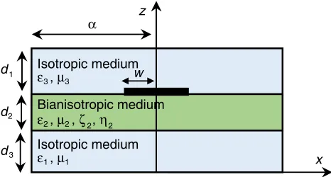
The studied bianisotropic substrate microstrip line structure is presented in Fig. 1. The upper and lower layers (region 1 and 3) are isotropic dielectrics.
α
d
d
d
1
2
3 x
z
w
Isotropic medium
ε 3, μ3
Bianisotropic medium
ε , μ , ζ , η Isotropic medium
ε 1, μ1
2 2 2 2
Figure 1. Geometry of the studied suspended microstrip line structure.
In general, bianisotropic media are characterized by the following constitutive relations [18].
B = [μ]H + ([χ] +j[ξ])√μ0ε0E
D= [ε]E + ([χ]−j[ξ])√μ0ε0H
(1a)
whereE,H,D andB are the electric field, magnetic field, electric flux density and magnetic flux density,
respectively. [ε] and [μ] are the electric permittivity and magnetic permeability tensors, respectively.
ε0 and μ0 are the free space permittivity and permeability, respectively. [χ] is the non-reciprocity
(Tellegen), tensor and [ξ] is the chirality (Pasteur) tensor.
The linear stationary dispersive bianisotropic materials can be described by the following constitutive relations in the frequency domain
D=ε0[ε(ω)]E +√ε0μ0[ξ(ω)]H
B =μ0[μ(ω)]H +√ε0μ0[η(ω)]E
(1b)
where the time dependence (ejwt) is assumed. In the Cartesian coordinate system, the tensors of the
relative permittivity [ε(ω)] and relative permeability [μ(ω)] are given by:
[ε(ω)] =
ε
xx εxy εxz
εyx εyy εyz
εzx εzy εzz
, [μ(ω)] =
μ
xx μxy μxz
μyx μyy μyz
μzx μzy μzz
(2a)
and the magnetoelectric tensors [ξ(ω)] and [η(ω)] are given by:
[ξ(ω)] =
ξxx ξxy ξxz
ξyx ξyy ξyz
ξzx ξzy ξzz
, [η(ω)] =
ηxx ηxy ηxz
ηyx ηyy ηyz
ηzx ηzy ηzz
(2b)
The bianisotropic medium is a generalization of the anisotropic and chiral media [19]. Different types of anisotropic media are possible: uniaxial, biaxial, gyrotropic,. . . , as it is possible to have only one nonzero element of the nine-element matrix [20]. In [14] and [21], a special case of the above magnetoelectric elements was treated. An important step in the distinction between anisotropic media comes through
splitting the constitutive parameter dyadic matrixx (x=ε, μ, ξ and η) into two parts, symmetric and
antisymmetric [22].
x=
xx xxy xxz
xyx xy xyz
xzx xzy xz
=
xx 0 0
0 xy 0
0 0 xz
symmetric→uniaxial,biaxialanisotropy
+
0
xxy xxz
xyx 0 xyz
xzx xzy 0
antisymmetric→gyrotropicanisotopy
(3a)
This can be simplified into:
x=xxu¯xu¯x+xyu¯yu¯y+xzu¯zu¯z
symmetric
+ x gu¯z×I
antisymmetric
(3b)
where:
xg=
0
xxy xxz
xyx 0 xyz
xzx xzy 0
(3c)
and I is the unit dyadic matrix.
The symmetric part of the dyad “x” has a principal axis along x, y or z direction, and these
elements determine the uniaxial and biaxial anisotropy. The other elements xg (antisymmetric) define
the gyrotropic anisotropy of the medium. When all the constitutive parameters are scalar, the medium is said to be biisotropic.
According to the gyrotropic bianisotropy of constitutive parametersξand η, it is possible to define
several medium types, depending on the form of the constitutive tensors in Equation (2). Some cases of
linear complex media are considered in [23–28]; in [24, 25], two cases: ξ=η= 0 andξ =−η, in [23–27],
the case: ξ =η= 0, and in [24, 28] the case: ξ =η.
2.2. Matrix Formulation
Calculation developments, starting from Maxwell’s equations and using the spectral domain GEMT, lead to a 1st order differential equation for the transverse electromagnetic field components as functions
of their derivatives in the ith region [6]:
∂
˜
f(i)(α, β, z)
∂z =
P(i)
4×4
˜
and:
˜
f(i)(α, β, z) =
⎡ ⎢ ⎢ ⎢ ⎢ ⎣
˜
Ex(i)(α, β, z) ˜
Ey(i)(α, β, z) ˜
Hx(i)(α, β, z) ˜
Hy(i)(α, β, z) ⎤ ⎥ ⎥ ⎥ ⎥
⎦ (4b)
[P] = jκ0{[A] + [B] [C][D]} (4c)
where
[A] =
⎡ ⎢ ⎣
−ηyx −ηyy −Z0μyx −Z0μyy
ηxx ηxy Z0μxx Z0μxy
Υ0εyx Υ0εyy ξyx ξyy
−Υ0εxx −Υ0εxy −ξxx −ξxy ⎤ ⎥
⎦=
[ηT] Z0[μT] −Υ0[εT] −[ξT]
(4d)
[B] = ⎡ ⎢ ⎣
−j(κ0ηyz+κx) −jωμ0μyz
j(κ0ηxz−κy) jωμ0μxz
jωε0εyz j(κ0ξyz−κx)
−jωε0εxz −j(κ0ξxz+κy) ⎤ ⎥
⎦=
⎡ ⎢ ⎢ ⎣
−(ηyz+κnx) −Z0μyz
ηxz−κny
Z0μxz
Υ0εyz (ξyz−κnx)
−Υ0εxz −
ξxz+κny
⎤ ⎥ ⎥
⎦ (4e)
[C] = −1
(εzzμzz−ξzzηzz)
Z0μzz ξzz
−ηzz −Υ0εzz
(4f)
[D] =
Υ0εxz Υ0εyz
ξxz−κny (ξyz+κnx)
−ηxz+κny
−(ηyz−κnx) −Z0μxz −Z0μyz
(4g)
whereκnx = κκx0 and κ
n
y = κκy0 are the normalized xandy wavenumber components, andZ0 =
1
Υ0 =
μ0
ε0 is the free space characteristic impedance.
[P] denotes a z-independent matrix. In all previous works [6, 7], matrix P is calculated explicitly,
while in this study it is kept in its matrix form, where the elements are derived from the constitutive relations. This matrix is the first form which characterizes the medium in our matrix formulation study. The elements of such a matrix are not necessarily developed; the matrix is inserted in its raw form. The general solution of Equation (4a) is given by:
⎡ ⎢ ⎣
Ex(z)
Ey(z)
Hx(z)
Hy(z)
⎤ ⎥
⎦= exp ([P]·z) ⎡ ⎢ ⎣
Ex(0)
Ey(0)
Hx(0)
Hy(0)
⎤ ⎥
⎦ (5)
which has a general solution of the form: ⎡
⎢ ⎣
Ex(z)
Ey(z)
Hx(z)
Hy(z)
⎤ ⎥
⎦=T(κx, κy, z)
⎡ ⎢ ⎣
Ex(0)
Ey(0)
Hx(0)
Hy(0)
⎤ ⎥
⎦ (6a)
and
˜
f(i)(α, β, z(i)) =T(κx, κy, z) ˜f(i)(α, β, z(i−1)) (6b)
According to Cayley-Hamilton theorem, the transition matrix is expressed under the following form
T(z) =c0I+c1P+c2P2+c3P3. (7)
where cj (j = 0,1,2,3) are scalar expansion coefficients that can be given by solving the Vandermode
linear algebraic system. According to Equation (6a), we realize the advantage of using this technique.
We notice that it is sufficient to know the transition matrices T(κx, κy, z) of the structure limit (upper
T(κx, κy, z) is calculated in the formulation of the GEMT by means of the Cayley Hamilton theorem in conjunction with Muller’s method to determine the complex function roots.
Muller’s method is a generalization of the secant method used to find real or complex zeros of a
function and is an iterative method which requires three starting points (p, f(p)), (p1,f(p1)), and (p2,
f(p2)). A parabola is made to fit the three points, then a quadratic formula is used to find a root of the
quadratic approximation for the next root. It is shown that close to a root Muller’s method converges more quickly than the secant method and almost as quickly as the Newton method.
2.3. Boundary Conditions and Green’s Matrix Tensor Evaluation
According to the conditions in the vicinity of a perfect conductor, the electric and magnetic field
components for regions z⊆[0, d1] andz⊆[d2, d3] are:
⎡ ⎢ ⎢ ⎣
Ex(z)
Ey(z)
Hx(z)
Hy(z)
⎤ ⎥ ⎥
⎦ = f(1)(α, β, z) = [L1]
˜
C1
˜
C4
(8a)
⎡ ⎢ ⎢ ⎣
Ex(z)
Ey(z)
Hx(z)
Hy(z)
⎤ ⎥ ⎥
⎦ = f(3)(α, β, z) = [L3]
˜
C2
˜
C3
(8b)
with
[L1] = ⎡ ⎢ ⎢ ⎢ ⎢ ⎢ ⎢ ⎢ ⎢ ⎢ ⎣
−αnγ0
ωε0 jβ
−βγ0
ωε0 −jαn
−jβcoth (γ0d1) −αnγ0
ωμ0
coth (γ0d1)
jαncoth (γ0d1) − β
ωμ0
coth (γ0d1) ⎤ ⎥ ⎥ ⎥ ⎥ ⎥ ⎥ ⎥ ⎥ ⎥ ⎦
(8c)
[L3] = ⎡ ⎢ ⎢ ⎢ ⎢ ⎢ ⎢ ⎢ ⎢ ⎢ ⎣
αnγ0
ωε0 jβ
βγ0
ωε0 −jαn
−jβcoth (γ0d3) αnγ0
ωμ0
coth (γ0d3)
jαncoth (γ0d3) β
ωμ0
coth (γ0d3) ⎤ ⎥ ⎥ ⎥ ⎥ ⎥ ⎥ ⎥ ⎥ ⎥ ⎦
(8d)
and
˜
C1 = C1sinh (γ0d1) (8e)
˜
C2 = C2sinh (γ0d3) (8f)
˜
C3 = C3sinh (γ0d3) (8g)
˜
C4 = C4sinh (γ0d1) (8h)
Applying the general solution of the GEMT and enforcing the boundary conditions imposed by the
conducting strips, we get: ⎡
⎢ ⎢ ⎢ ⎢ ⎣
˜ Ex(3)
˜ Ey(3)
˜ Hx(3)
˜ Hy(3)
⎤ ⎥ ⎥ ⎥ ⎥
⎦−
⎡ ⎢ ⎢ ⎢ ⎢ ⎣
˜ Ex(2)
˜ Ey(2)
˜ Hx(2)
˜ Hy(2)
⎤ ⎥ ⎥ ⎥ ⎥
⎦=
⎡ ⎢ ⎢ ⎢ ⎣
0 0 −J˜(2)
y
˜ Jx(2)
⎤ ⎥ ⎥ ⎥
According to Equation (9), we obtain the matrix equation which relates the transverse components of the electric and magnetic fields to the transverse current densities [6].
[T] [L1]
˜
C1
˜
C4
= [L3]
˜
C2
˜
C3
+
⎡ ⎢ ⎢ ⎣
0 0 ˜
Jy
−J˜x ⎤ ⎥ ⎥
⎦ (10a)
[L](4,2) = [T]·[L1](4,2) (10b)
[L](4,2)·
˜
C1
˜
C4
= [L3](4,2)·
˜
C2
˜
C3
+
⎡ ⎢ ⎢ ⎣
0 0 ˜
Jy
−J˜x ⎤ ⎥ ⎥
⎦. (10c)
We denote by [L] and [L3] the transfer matrices for the structures which contain the layers with
(0≤z≤d1) and (d2≤z≤d3).
[FM] ⎡ ⎢ ⎢ ⎣
˜
C1
˜
C4
˜
C2
˜
C3
⎤ ⎥ ⎥
⎦ =
⎡ ⎢ ⎢ ⎣
0 0 ˜
Jy
−J˜x ⎤ ⎥ ⎥
⎦ (11a)
[FM](4,4) = L(4,2) L3(4,2) (11b)
Using Cramer’s rule for the determination of the constants obtained by enforcing the boundary conditions in the air-dielectric interface, we get the following matrix form for these constants:
[C1] =
F M(1,1) F M(1,2) F M(1,4)
F M(2,1) F M(2,2) F M(2,4)
F M(4,1) F M(4,2) F M(4,4)
(12a)
[C2] =
F M(1,1) F M(1,2) F M(1,4)
F M(2,1) F M(2,2) F M(2,4)
F M(3,1) F M(3,2) F M(3,4)
(12b)
[C3] =
F M(1,1) F M(1,2) F M(1,3)
F M(2,1) F M(2,2) F M(2,3)
F M(4,1) F M(4,2) F M(4,3)
(12c)
[C4] =
F M(1,1) F M(1,2) F M(1,3)
F M(2,1) F M(2,2) F M(2,3)
F M(3,1) F M(3,2) F M(4,3)
(12d)
where [C1] is obtained by deleting the 3rdrow and 3rdcolumn of [FM](4,4), [C2] obtained by deleting the
4th row and 3rd column of [FM](4,4), [C3] obtained by deleting the 3rd row and 4th column of [FM](4,4),
[C4] obtained by deleting the 4th row and 4th column of [FM](4,4), and [C1] obtained by deleting the
3rd row and 3rd column of [FM](4,4).
This matrix formulation exhibits a compact form with the advantage of being easily integrated in the calculation code.
At the air-dielectric interface z = d2, the continuity of the field tangential components has to be
satisfied. By determining the expressions of the constants [C1], [C2], [C3] and [C4], the expressions of
the electric and magnetic fields are evaluated at the interface air-dielectric. Hence, the novel matrix
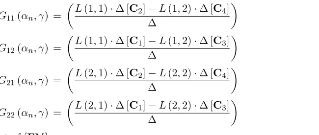
form of the elements of the Green tensor Gij(αn, γ) is obtained according to the following system of
equations.
˜
Ex = G11(αn, γ) ˜jx+G12(αn, γ) ˜jy (13a)
˜
where
G11(αn, γ) =
L(1,1)·Δ [C2]−L(1,2)·Δ [C4]
Δ
(13c)
G12(αn, γ) =
L(1,1)·Δ [C1]−L(1,2)·Δ [C3]
Δ
(13d)
G21(αn, γ) =
L(2,1)·Δ [C2]−L(2,2)·Δ [C4]
Δ
(13e)
G22(αn, γ) =
L(2,1)·Δ [C1]−L(2,2)·Δ [C3]
Δ
(13f)
where Δ is the determinant of [FM](4,4).
2.4. Resolution of the System
By enforcing the boundary conditions imposed on the field components and the current distributions at the air-dielectric interface, the integral equations are converted into a homogeneous system of linear
equations. The resolution of the equation det(γ) = 0 is carried out using the spectral domain MoM and
Galerkin’s procedure [6, 8, 17]. For lossy media, a complex propagation constantγ =α+jβis expected.
3. RESULTS AND DISCUSSION
3.1. Validation of Results
Figures 2 and 3 show the case study of 2 and 3-layer structures (Fig. 1) compared with results reported in literature [16, 29]. Our obtained results are in good agreement with the studied cases. A slight shift that does not exceed 8% is observed which is mainly due to the consideration of the dielectric losses.
5 10 15 20
3 6 9 12
ε =2.35
f (GHz) 5 10 15 20
0.0 0.1 0.2 0.3 0.4
f (GHz)
()
2x10
-3
r
α/κ
0
()
2
β/κ
0
(a) (b)
ε =2.35 [30]
ε =9.40
ε =9.40 [29]
ε =20.0
ε =20.0 [29]
r r r r r
ε r=2.53
ε =9.35
ε =20
r r
Figure 2. (a) (κβ 0)
2 ratio, and (b) (α
κ0)2 ratio of the suspended microstrip line structure for different
values ofεr. (a= 10 mm, d1 = 4.5 mm,d2= 1 mm, d3 = 4.5 mm,w= 1 mm).
10 20 30 40 50 0
3 6 9 12 15 18
f (GHz) 10 20 30 40 50
0,0 0,1 0,2 0,3 0,4 0,5 0,6
()
2x10
-3
α/κ
0
()
2
β/κ
0
f (GHz)
(a) (b)
ε r=2.35 ε =2.35 [16] ε =9.40 ε =9.40 [16] ε =20.0 ε =20.0 [16]
r
r
r r
r
ε r=2.53 ε =9.35 ε =20
r
r
Figure 3. (a) (κβ 0)
2 ratio, and (b) (α
κ0)
2 ratio of the microstrip for different values ofε
r. (a= 12.7 mm,
d1 = 11.43 mm, d2 = 0.5 mm,d3 = 0 mm, w= 0.5 mm).
10 20 30 40 50
1,4 1,6 1,8 2,0 2,2 2,4
2,6 ξxx=0 [16]
(isotropic case)
xx=0.8r
xx=1.0
ε r
xx=1.2r
xx=-0.8r
xx=-1.0r
xx=-1.2r
xx=j 0.8r
xx=j 1.0r
xx=j 1.2r
xx=-j 0.8r
xx=-j 1.0r
xx=-j 1.2r
f (GHz)
10 20 30 40 50
1,80 1,84 1,88 1,92
1,96 xx=0 [16]
(isotropic case)
xx=0.8r
xx=1.0r
xx=1.2r
xx=-0.8r
xx=-1.0r
xx=-1.2r
xx=j 0.8r
xx=j 1.0r
xx=j 1.2r
xx=-j 0.8r
xx=-j 1.0r
xx=-j 1.2r
10 20 30 40 50
0,00000 0,00005 0,02 0,03 0,04
0,05 xx=0
(isotropic case)
xx=0.8r
xx=1.0r
xx=1.2r
xx=-0.8r
xx=-1.0r
xx=-1.2r
xx=j 0.8r
xx=j 1.0r
xx=j 1.2r
xx=-j 0.8r
xx=-j 1.0r
xx=-j 1.2r
()
2
α/κ
0
()
2
β/κ
0
()
2
β/κ
0
ξ ξ ξ ξ ξ ξ ξ ξ ξ ξ ξ ξ
ξ
ξ ξ ξ ξ ξ ξ ξ ξ ξ ξ ξ ξ
ξ
ξ ξ ξ ξ ξ ξ ξ ξ ξ ξ ξ ξ
f (GHz)
ε ε ε ε ε ε ε ε ε ε ε
ε ε ε ε ε ε ε ε ε ε ε ε
ε ε ε ε ε ε ε ε ε ε ε ε
f (GHz)
(a)
(b)
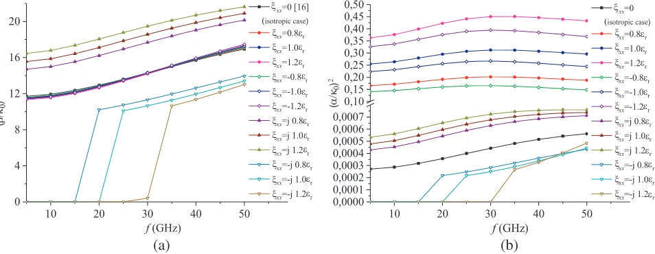
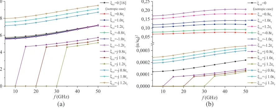
Figure 4. Effect of the chirality ξxx on the (a) (κβ0)2 ratio and (b) (κα0)2 ratio of the microstrip.
3.2. Effect of the Chirality on the Complex Propagation Constant
The following figures present the effect of the chirality parameter ξ and η of a monolayer microstrip
line structure (d3 = 0 mm in Fig. 1). Initially we examine the effect of the axial chirality element by
element.
The values of the magnetoelectric elements, whether they are real or imaginary, positive or negative, directly affect the effective constant as well as the losses.
According to Fig. 4(a), the notion of non-reciprocity is remarkable when changing the sign of the
purely imaginary magnetoelectric element ξxx, with an increase in (β/κ0)2 when imaginary
positive-valuedξxx increases and a decrease when imaginary negative-valuedξxx decreases. This effect reversed
with respect to (α/κ0)2 parameter, which is clearly illustrated by Fig. 4(c).
The increase in real values of ξxx leads to a slight decrease in (β/κ0)2 and a significant increase in
the ratio (α/κ0)2 (Figs. 4(a) and (b)). Real positive values of ξxx have more effect than negative ones;
10 20 30 40 50
0 2 4 6 8
10 xx=0 [16]
(isotropic case)
xx=0.8r
xx=1.0
ε r
xx=1.2r
xx=-0.8r
xx=-1.0r
xx=-1.2r
xx=j 0.8r
xx=j 1.0r
xx=j 1.2r
xx=-j 0.8r
xx=-j 1.0r
xx=-j 1.2r
f (GHz) 10 20 30 40 50
0,0000 0,0001 0,0002 0,0003 0,05 0,10 0,15 0,20
0,25 xx=0
(isotropic case)
xx=0.8r
xx=1.0r
xx=1.2r
xx=-0.8r
xx=-1.0r
xx=-1.2r
xx=j 0.8r
xx=j 1.0r
xx=j 1.2r
xx=-j 0.8r
xx=-j 1.0r
xx=-j 1.2r
f (GHz) ξ ξ ξ ξ ξ ξ ξ ξ ξ ξ ξ ξ ξ ξ ξ ξ ξ ξ ξ ξ ξ ξ ξ ξ ξ ξ ε ε ε ε ε ε ε ε ε ε ε ε ε ε ε ε ε ε ε ε ε ε ε () 2 α/κ 0 () 2 β/κ 0 (a) (b)
Figure 5. Effect of the chirality ξxx on (a) the (κβ0)2 ratio and (b) the (κα0)2 ratio of the microstrip.
(a= 12.7 mm, d1 = 11.43 mm, d2 = 0.5 mm,d3 = 0 mm, w= 0.5 mm, εr= 9.4).
10 20 30 40 50
0 4 8 12 16 20 xx =0 [16]
(isotropic case)
xx=0.8r
xx=1.0r
xx=1.2r
xx=-0.8r
xx=-1.0r
xx=-1.2r
xx=j 0.8r
xx=j 1.0r
xx=j 1.2r
xx=-j 0.8r
xx=-j 1.0r
xx=-j 1.2r
f (GHz) 10 20 30 40 50
0,0000 0,0001 0,0002 0,0003 0,0004 0,0005 0,0006 0,0007 0,10 0,15 0,20 0,25 0,30 0,35 0,40 0,45
0,50 xx=0
(isotropic case)
xx=0.8r
xx=1.0r
xx=1.2r
xx=-0.8r
xx=-1.0r
xx=-1.2r
xx=j 0.8r
xx=j 1.0r
xx=j 1.2r
xx=-j 0.8r
xx=-j 1.0r
xx=-j 1.2r
f (GHz) () 2 α/κ 0 () 2 β/κ 0 ξ ξ ξ ξ ξ ξ ξ ξ ξ ξ ξ ξ ξ ξ ξ ξ ξ ξ ξ ξ ξ ξ ξ ξ ξ ξ (a) (b) ε ε ε ε ε ε ε ε ε ε ε ε ε ε ε ε ε ε ε ε ε ε ε ε
Figure 6. Effect of the chirality ξxx on (a) the (κβ 0)
2 ratio and (b) the (α
κ0)2 ratio of the microstrip.
these effects on (α/κ0)2 and (β/κ0)2 are reversed with respect to the sign of the parameterξxx.
Figs. 4, 5 and 6 illustrate the effect of chirality for εr = 2.53, 9.4 and 20, respectively. We observe
that the increase inεr induces an increase in the chirality effect (ξxx is kept constant) on both (α/κ0)2
and (β/κ0)2 parameters. In particular, for a negative imaginary magnetoelectric element, we observe
a delayed appearance of the fundamental mode increasingly with the increase εr (5 GHz for εr = 2.53,
15 GHz forεr= 9.4 and 20 GHz for εr= 20). The effective permittivity starts approximately from the
reference (isotropic case +∼= [0.5∗(εr+ 1) + Δf(εr,ξxx)]) in all treated cases.
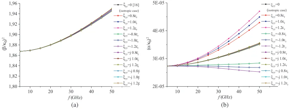
Regarding the magnetoelectric elementξyy(Fig. 7), its effect on the parameters (α/κ0)2and (β/κ0)2
is insignificant, due to the choice of the geometrical orientation of the treated structure (Fig. 1). Figs. 8
and 9 present the combined effect of ξzz with εr = 2.53 and 9.4, respectively, which is marked by
almost identical effects relative to ξzz. The magnetoelectric elements ηzz have the same effect as that
of parameter (−ξzz) as illustrated by Figs. 10, 11 and 12.
10 20 30 40 50
1,80 1,82 1,84 1,86 1,88 1,90 1,92 1,94
1,96 yy=0 [16]
(isotropic case)
yy=0.8r
yy=1.0r
yy=1.2r
yy=-0.8r
yy=-1.0r
yy=-1.2r
yy=j 0.8r
yy=j 1.0r
yy=j 1.2r
yy=-j 0.8r
yy=-j 1.0r
yy=-j 1.2r
f (GHz) 10 20 30 40 50
2E-05 3E-05 4E-05
5E-05 yy=0
(isotropic case)
yy=0.8r
yy=1.0r
yy=1.2r
yy=-0.8r
yy=-1.0r
yy=-1.2r
yy=j 0.8r
yy=j 1.0r
yy=j 1.2r
yy=-j 0.8r
yy=-j 1.0r
yy=-j 1.2r
f (GHz)
() 2 α/κ 0 () 2 β/κ 0 ξ ε ξ ξ ξ ξ ξ ξ ξ ξ ξ ξ ξ ξ ε ε ε ε ε ε ε ε ε ε ε ξ ξ ξ ξ ξ ξ ξ ξ ξ ξ ξ ξ ξ ε ε ε ε ε ε ε ε ε ε ε ε (a) (b)
Figure 7. Effect of the chirality ξyy on (a) the (κβ 0)
2 ratio and (b) the (α
κ0)2 ratio of the microstrip.
(a= 12.7 mm, d1 = 11.43 mm, d2 = 0.5 mm,d3 = 0 mm, w= 0.5 mm, εr= 2.53).
10 20 30 40 50
1,4 1,6 1,8 2,0 2,2 2,4
2,6 zz=0 [16]
(isotropic case)
zz=0.8r
zz=1.0r
zz=1.2r
zz=-0.8r
zz=-1.0r
zz=-1.2r
zz=j 0.8r
zz=j 1.0r
zz=j 1.2r
zz=-j 0.8r
zz=-j 1.0r
zz=-j 1.2r
f (GHz) 10 20 30 40 50
0,00000 0,00005 0,02 0,03 0,04
0,05 zz=0
(isotropic case)
zz=0.8r
zz=1.0r
zz=1.2r
zz=-0.8r
zz=-1.0r
zz=-1.2r
zz=j 0.8r
zz=j 1.0r
zz=j 1.2r
zz=-j 0.8r
zz=-j 1.0r
zz=-j 1.2r
f (GHz)
() 2 α/κ 0 () 2 β/κ 0 ξ ε ξ ξ ξ ξ ξ ξ ξ ξ ξ ξ ξ ξ ε ε ε ε ε ε ε ε ε ε ε ξ ε ξ ξ ξ ξ ξ ξ ξ ξ ξ ξ ξ ξ ε ε ε ε ε ε ε ε ε ε ε (a) (b)
Figure 8. Effect of the chirality ξzz on (a) the (κβ 0)
2 ratio and (b) the (α
κ0)2 ratio of the microstrip.
10 20 30 40 50 0 2 4 6 8
10 zz=0 [16]
(isotropic case)
zz=0.8r
zz=1.0r
zz=1.2r
zz=-0.8r
zz=-1.0r
zz=-1.2r
zz=j 0.8r
zz=j 1.0r
zz=j 1.2r
zz=-j 0.8r
zz=-j 1.0r
zz=-j 1.2r
f (GHz) 10 20 30 40 50
0,0000 0,0001 0,0002 0,0003 0,05 0,10 0,15 0,20
0,25 zz=0
(isotropic case)
zz=0.8r
zz=1.0r
zz=1.2r
zz=-0.8r
zz=-1.0r
zz=-1.2r
zz=j 0.8r
zz=j 1.0r
zz=j 1.2r
zz=-j 0.8r
zz=-j 1.0r
zz=-j 1.2r
() 2 α/κ 0 () 2 β/κ 0
f (GHz)
ξ ε ξ ξ ξ ξ ξ ξ ξ ξ ξ ξ ξ ξ ε ε ε ε ε ε ε ε ε ε ε ξ ε ξ ξ ξ ξ ξ ξ ξ ξ ξ ξ ξ ξ ε ε ε ε ε ε ε ε ε ε ε (a) (b)
Figure 9. Effect of the chirality ξzz on (a) the (κβ 0)
2 ratio and (b) the (α
κ0)2 ratio of the microstrip.
(a= 12.7 mm, d1 = 11.43 mm, d2 = 0.5 mm,d3 = 0 mm, w= 0.5 mm, εr= 9.4).
10 20 30 40 50
0 4 8 12 16
20 (isotropic casezz=0 [16])
zz=0.8r
zz=1.0r
zz=1.2r
zz=-0.8r
zz=-1.0r
zz=-1.2r
zz=j 0.8r
zz=j 1.0r
zz=j 1.2r
zz=-j 0.8r
zz=-j 1.0r
zz=-j 1.2r
f (GHz) 10 20 30 40 50
0,0000 0,0001 0,0002 0,0003 0,0004 0,0005 0,0006 0,0007 0,10 0,15 0,20 0,25 0,30 0,35 0,40 0,45
0,50 zz=0
(isotropic case)
zz=0.8r
zz=1.0r
zz=1.2r
zz=-0.8r
zz=-1.0r
zz=-1.2r
zz=j 0.8r
zz=j 1.0r
zz=j 1.2r
zz=-j 0.8r
zz=-j 1.0r
zz=-j 1.2r
() 2 α/κ 0 () 2 β/κ 0 ξ ε ξ ξ ξ ξ ξ ξ ξ ξ ξ ξ ξ ξ ε ε ε ε ε ε ε ε ε ε ε ξ ε ξ ξ ξ ξ ξ ξ ξ ξ ξ ξ ξ ξ ε ε ε ε ε ε ε ε ε ε ε
f (GHz)
(a) (b)
Figure 10. Effect of the chirality ξzz on (a) the (κβ0)2 ratio and (b) the (κα0)2 ratio of the microstrip.
(a= 12.7 mm, d1 = 11.43 mm, d2 = 0.5 mm,d3 = 0 mm, w= 0.5 mm, εr= 20).
10 20 30 40 50
0 2 4 6 8
10 xx=0 [16]
(isotropic case)
xx=0.8r
xx=1.0r
xx=1.2r
xx=-0.8r
xx=-1.0r
xx=-1.2r
xx=j 0.8r
xx=j 1.0r
xx=j 1.2r
xx=-j 0.8r
xx=-j 1.0r
xx=-j 1.2r
f (GHz) 10 20 30 40 50
0,0000 0,0001 0,0002 0,0003 0,05 0,10 0,15 0,20
0,25 xx=0
(isotropic case)
xx=0.8r
xx=1.0r
xx=1.2r
xx=-0.8r
xx=-1.0r
xx=-1.2r
xx=j 0.8r
xx=j 1.0r
xx=j 1.2r
xx=-j 0.8r
xx=-j 1.0r
xx=-j 1.2r
f (GHz)
() 2 α/κ 0 () 2 β/κ 0 ξ ε ξ ξ ξ ξ ξ ξ ξ ξ ξ ξ ξ ξ ε ε ε ε ε ε ε ε ε ε ε ξ ε ξ ξ ξ ξ ξ ξ ξ ξ ξ ξ ξ ξ ε ε ε ε ε ε ε ε ε ε ε (a) (b)
Figure 11. Effect of the chirality ηxx on (a) the (κβ0)2 ratio and (b) the (κα0)2 ratio of the microstrip.
10 20 30 40 50 0
2 4 6 8
10 zz=0 [16]
(isotropic case)
zz=0.8r
zz=1.0r
zz=1.2r
zz=-0.8r
zz=-1.0r
zz=-1.2r
zz=j 0.8r
zz=j 1.0r
zz=j 1.2r
zz=-j 0.8r
zz=-j 1.0r
zz=-j 1.2r
f (GHz) 10 20 30 40 50
0,0000 0,0001 0,0002 0,0003 0,05 0,10 0,15 0,20
0,25 zz=0
(isotropic case)
zz=0.8r
zz=1.0r
zz=1.2r
zz=-0.8r
zz=-1.0r
zz=-1.2r
zz=j 0.8r
zz=j 1.0r
zz=j 1.2r
zz=-j 0.8r
zz=-j 1.0r
zz=-j 1.2r
f (GHz)
()
2
α/κ
0
()
2
β/κ
0
ξ
ε ξ ξ ξ ξ ξ ξ ξ ξ ξ ξ ξ ξ
ε ε ε ε ε ε ε ε ε ε ε
ξ
ε ξ ξ ξ ξ ξ ξ ξ ξ ξ ξ ξ ξ
ε ε ε ε ε ε ε ε ε ε ε
(a) (b)
Figure 12. Effect of the chirality ηzz on (a) the (κβ0)2 ratio and (b) the (κα0)2 ratio of the microstrip.
(a= 12.7 mm, d1 = 11.43 mm, d2 = 0.5 mm,d3 = 0 mm, w= 0.5 mm, εr= 9.4).
4. CONCLUSION
A detailed analytical development of Maxwell’s equations for the characterization of a complex medium multilayer transmission line structure is presented. This study is based on the Generalized Exponential Matrix Technique combined with the method of moments and Galerkin’s procedure. The analytical formulation of the problem is carried out through a matrix formulation approach that excludes all calculation complexities and avoids excessive developments of intermediate elements, in particular Equations (4c) and (13c)–(13f). This results in a compact matrix form of the Green’s tensor. This matrix formulation approach facilitates the characterization study of a complex medium structure with full tensors of the constitutive parameters with the consideration, for the first time, of the substrate dielectric losses. A multitude of diverse and interesting results has been obtained, which are consistent with the literature. Among them, only the cases of exploitable applications have been interpreted.
ACKNOWLEDGMENT
The authors are thankful to the anonymous reviewers for making constructive criticisms on the work, which essentially helped to raise the status of manuscript.
REFERENCES
1. Peri´c, M., S. Ili´c, S. Aleksi´c, N. Rai˘cevi´c, M. Bichurin, A. Tatarenko, and R. Petrov, “Covered
microstrip line with ground planes of finite width,” Facta Universitatis Series: Electronics and
Energetics, Vol. 27, No. 4, 589–600, Dec. 2014.
2. Tae, H. S., K. S. Oh, H. L. Lee, W. I. Son, and J. W. Yu, “Reconfigurable 1 : 4 power divider
with switched impedance matching circuits,” IEEE Microwave and Wireless Components Letters,
Vol. 22, No. 2, 64–66, Feb. 2012.
3. Koul, S. K. and B. Bhat, “Inverted microstrip and suspended microstrip with anisotropic
substrates,”Proceedings of the IEEE, Vol. 70, No. 10, 1230–1231, Oct. 1982.
4. Tsalamengas, J. L., “Interaction of electromagnetic waves with general bianisotropic slabs,” IEEE
5. Umashankar, K., A. Taflove, and S. Rao, “Electromagnetic scattering by arbitrary shaped
three-dimensional homogeneous lossy dielectric objects,” IEEE Transactions on Antennas and
Propagation, Vol. 34, No. 6, 758–766, 1986.
6. Yin, W.-Y., L.-W. Li, and I. Wollf, “The compatible effects of gyrotropy and chirality in biaxially
bianisotropic chiral-and chiroferrite-ferrite microstrip line structure,” International Journal of
Numerical Modelling: Electronic Networks, Devices and Fields, Vol. 12, 209–227, 1999.
7. Weiglhofer, W. S., “A perspective on bianisotropy and Bianisotropics’ 97,” International Journal
of Applied Electromagnetics and Mechanics, Vol. 9, No. 2, 93–101, 1998.
8. Zebiri, C., D. Sayad, S. Daoudi, and F. Benabdelaziz, “Microstrip line printed on a bianisotropic
medium,” International Conference on Advanced Communication Systems and Signal Processing,
ICOSIP-2015, 111–120, 2015.
9. Heindl, R., H. Srikanth, S. Witanachchi, P. Mukherjee, T. Weller, A. S. Tatarenko, and G. Srinivasan, “Structure, magnetism, and tunable microwave properties of pulsed laser deposition
grown barium ferrite/barium strontium titanate bilayer films,” J. Appl. Phys., Vol. 101, No. 09,
09M503, 2007.
10. Tatarenko, A. S., D. V. Snisarenko, and M. Bichurin, “Modeling of magnetoelectric microwave
devices,” Facta Universitatis, Series: Electronics and Energetics, Vol. 30, No. 3, 285–293, 2017.
11. Zebiri, C., F. Benabdelaziz, and M. Lashab, “Bianisotropic superstrate effect on rectangular
microstrip patch antenna parameters,” META’12, 2012.
12. Herman, W.-N., “Polarization eccentricity of the transverse field for modes in chiral core planar
waveguides,” Journal of the Optical Society of America A: Optics, Image Science and Vision,
Vol. 18, No. 11, 2806–2818, 2001.
13. Engheta, N., “The theory of chirostrip antennas,” Proceedings of the 1988 URSI International
Radio Science Symposium, 213, Syracuse, New York, 1988.
14. Zebiri, C., M. Lashab, and F. Benabdelaziz, “Effect of anisotropic magneto-chirality on the
characteristics of a microstrip resonator,” IET Microwaves, Antennas Propagation, Vol. 4, No. 4,
446–452, 2010.
15. Hillion, P., “Harmonic plane wave propagation in anisotropic chiral media,” International Journal
of Applied Electromagnetics and Mechanics, Vol. 28, No. 3, 337–350, 2008.
16. Khodja, A., M. L. Tounsi, M. C. E. Yagoub, and S. Gaoua, “Full-wave analysis of the anisotropy
effect in unilateral planar transmission lines by integral method,” SETIT 2005, 3rd International
Conference: Sciences of Electronic Technologies of Information and Telecommunications, Mar. 27–
31, 2005.
17. Daoudi, S., F. Benabdelaziz, and C. Zebiri, “Spectral-domain analysis of finline printed on chiral and ferrite substrates using the generalized exponential technique combined with Galerkin’s
method,” European Journal of Science and Technology, No. 8, 53–56, Sep. 2016. (Special Issue of
the 2nd International Conference on Computational and Experimental Science and Engineering
(ICCESEN-2015), Antalya, Turkey, Oct. 14–19, 2015.)
18. Aib, S., F. Benabdelaziz, C. Zebiri, and D. Sayad, “Propagation in diagonal anisotropic
chirowaveguides,” Advances in OptoElectronics, Vol. 2017, 2017.
19. Lindell, V., A. H. Sihvola, S. A. Tretyskov, and A. J. Vitanen, Electromagnetic Waves in Chiral
and Bi-isotropic Media, Altech House, Norwood, MA, 1994.
20. Wang, S. Y., W. Y. Yin, L. Zhou, J. Chen, X. Q. Gu, and L. F. Qiu, “THz wave interaction
with planar structures consisting of multilayer graphene sheets and bianisotropic slabs,” IEEE
International Wireless Symposium (IWS), 1–4, 2014.
21. Zebiri, C., F. Benabdelaziz, and M. Lashab, “Complex media parameter effect: On the input
impedance of rectangular microstrip antenna,” IEEE International Conference Complex Systems
(ICCS), 1–4, 2012.
22. Zebiri, C., M. Lashab, and F. Benabdelaziz, “Asymmetrical effects of bi-anisotropic
substrate-superstrate sandwich structure on patch resonator,” Progress In Electromagnetics Research B,
23. Tretyakov, S. A. and A. A. Sochava, “Proposed composite material for nonreflecting shields and
antenna radoms,”Electron. Lett., Vol. 29, No. 12, 1048–1049, 1993.
24. Dmitriev, V., “Table of the second rank constitutive tensors for linear homogeneous media described
by the point magnetic groups of symmetry,”Progress In Electromagnetic Research, Vol. 28, 43–95,
2000.
25. Yin, W.-Y., “Linear complex media,” Encyclopedia of RF and Microwave Engineering, 694–717,
John Wiley, New York, 2005.
26. Zebiri, C., M. Lashab, and F. Benabdelaziz, “Rectangular microstrip antenna with uniaxial
bi-anisotropic chiral substrate-superstrate,” IET Microwaves, Antennas Propagation, Vol. 5, No. 1,
17–29, Jan. 2011.
27. Sayad, D., F. Benabdelaziz, C. Zebiri, S. Daoudi, and R. A. Abd-Alhameed, “Spectral domain analysis of gyrotropic anisotropy chiral effect on the input impedance of a printed dipole antenna,”
Progress In Electromagnetics Research M, Vol. 51, 1–8, 2016.
28. Zebiri, C., S. Daoudi, F. Benabdelaziz, M. Lashab, D. Sayad, N. T. Ali, and R. A. Abd-Alhameed, “Gyro-chirality effect of bianisotropic substrate on the operational of rectangular microstrip patch
antenna,” International Journal of Applied Electromagnetics and Mechanics, Vol. 51, No. 3, 249–
260, 2016.
29. Khodja, A., M. C. E. Yagoub, R. Touhami, and H. Baudrand, “Improved numerical modal
technique for fast and accurate modeling of transmission planar structures: Application to
microstrip line,” 2015 International Conference on Synthesis, Modeling, Analysis and Simulation
Methods and Applications to Circuit Design (SMACD), 1–4, IEEE, 2015.
30. Polichronakis, I. P. and S. S. Kouris, “Computation of the dispersion characteristics of a shielded
suspended substrate microstrip line,” IEEE Transactions on Microwave Theory and Techniques,