Simulating Underwater Electric Field Signal of Ship Using the
Boundary Element Method
Xiangjun Wang1, Qinglin Xu1, *, Jianchun Zhang1, and Fangjun Liu2
Abstract—Seawater conductivity is an important factor that affects the corrosion electric field of ship. A three-dimensional boundary element method (3D-BEM) combined with nonlinear polarization curve was employed to investigate the influence of seawater conductivity on the corrosion electrostatic field. Numerical simulation results show that the electric field distribution is only slightly influenced by the conductivity. However, the intensity decreases with the increases of conductivity. The simulation results of the BEM model were compared with the results of the equivalent electric dipole model, and the results obtained by the two methods had high similarity, which demonstrated that the BEM model was effective. The former is a more convenient and concise modeling method that can better reflect the distribution characteristics of ship’s corrosion electric field than the electric dipole model.
1. INTRODUCTION
The underwater signals (mainly including acoustic, magnetic and electric field) of warships have posed a great threat to their viability [1]. Since the World War II, acoustic signal and magnetic signal have been widely used as underwater signal sources in naval operations [2], but electric field signals generated by corrosion and anti-corrosion have not been used in the field of underwater detection and positioning. However, with the continuous development of underwater electric field detection technology, corrosion electric field has become the signal source of new mine warfare weapon [3]. In order to improve the survivability of naval vessels, the corrosion electric field must be suppressed or eliminated [4–6], and the analysis of the distribution characteristics of corrosion electric field under water is the basis for the above research.
The equivalent electric dipole model of corrosion electric field of ship was established, and the electromagnetic field generated by horizontal and vertical electric dipoles in multilayer medium was analyzed [7, 8]. Furthermore, the effect of environmental factors such as seabed conductivity or seawater conductivity, depth and temperature on underwater electric field was studied [9–11]. The boundary element method is a method based on the weighted residual method, which converts the boundary value problem into a boundary integral equation problem and then uses the finite element discrete technique to construct linear equations [12]. BEM was applied to anticorrosion research of offshore engineering structures in the early 1980s [13, 14]. Nowadays, it has been widely used in the simulation of cathodic protection system optimization of various marine structural parts such as oil rigs, submarine pipelines and ships [15–17]. Wu et al. [18] optimized the auxiliary anode position and output current of impressed current cathodic protection (ICCP) by BEM to reduce the corrosion electric field of ship effectively.
Electric dipole moment is mainly obtained through experience and literature when using electric dipole model to simulate the ship’s corrosion electric field distribution, it will change significantly when
Received 27 September 2018, Accepted 31 October 2018, Scheduled 23 November 2018 * Corresponding author: Qinglin Xu ([email protected]).
1 College of Electrical Engineering, Naval University of Engineering, Wuhan 430033, China.2Academy of Mathematics and Computer
the area and position of damage undergo changes, at this time, it is difficult to accurately obtain the corresponding electric dipole moment that affects the calculation accuracy of corrosion electric field directly. In this paper, the 3-D BEM was employed to establish the corrosion electrostatic field model of submarine, and the nonlinear polarization curve was taken as boundary condition of the model. The influence of seawater conductivity on the corrosion electric field of ship was studied, and the electric field distribution with different seawater conductivity was obtained. The results of the BEM model used in this paper were compared with the simulation results of the equivalent electric dipole model.
2. BASIC EQUATIONS AND BOUNDARY ELEMENT FORMULATION
The governing equation and boundary conditions for the 3-D corrosion electric field are shown in Fig. 1 [19]. The uniform seawater medium is represented by Ω, and the boundary of the seawater domain is composed of S1, S2,S3a and S3c in the picture. The potential distribution of seawater domain and electrode surface is in accordance with the following Laplace equation and boundary conditions [13]:
∇2u= ∂2u
∂2x +
∂2u ∂2y +
∂2u
∂2z = 0 (1)
⎧ ⎪ ⎪ ⎪ ⎪ ⎪ ⎪ ⎪ ⎨ ⎪ ⎪ ⎪ ⎪ ⎪ ⎪ ⎪ ⎩
u=u0 (Constant potential boundary)
q= ∂u
∂n =q0 (Constant current boundary) q= ia
σ =
1
σfa(ua) (Anodic polarization boundary) q= ic
σ =
1
σfc(uc) (Cathodic polarization boundary)
(2)
whereuis the potential of seawater medium and electrode surface; nis the unit outward normal to the surface; q is the normal derivative of potential (intensity of electric field); u0 and q0 are the constant values ofuandq at the boundaries ofS1 andS2, respectively;σis the seawater conductivity;fa(ua) and
fc(uc) represent the anodic polarization equation and the cathodic polarization equation, respectively.
Figure 1. Governing equation and boundary condition for applying BEM to corrosion electric field.
The equivalent boundary integral equation (1) is:
ciui+
S
u(ξ)∂u
∗(i, ξ)
∂n(ξ) dS =
S
q(ξ)u∗(i, ξ)dS (3)
ci = 0 when the field pointi is outside the domain of Ω;u(ξ) and q(ξ) represent potential and normal derivative of potential at any point on the boundary, respectively; u∗(i, ξ) is the basic solution to the three-dimensional static electromagnetic field problem, and its expression is:
u∗(i, ξ) = 1
4πr (4)
where r is the distance between i and ξ. In order to solve the boundary integral Equation (3), the boundary is divided into several units, recording the potential and normal derivative of potential of the nodes as following:
{u}= (u1, u2,· · ·uN)T {q}= (q1, q2,· · ·qN)T
(5)
The discrete equation of boundary integral equation can be derived as:
[H]{u}= [G]{q} (6)
where [H] and [G] are both N ×N coefficient matrices, andN is the total number of boundary nodes. The Taylor expansion of the current density ic in any point of cathodic surface at ¯uc by the nonlinear polarization equation is:
ic =ic(¯uc) + dic
duc |u¯c(uc−u¯c) + 1 2!
d2ic
du2
c |u¯c(uc−u¯c)
2+· · · (7)
Ignoring high-order items, only the first two items are:
ic =ic(¯uc) + (uc−u¯c)ic(¯uc) (8) or
qc = 1
σ[ic(¯uc) + (uc−u¯c)i
c(¯uc)] (9)
In the same way,
qa= 1
σ[ia(¯ua) + (ua−u¯a)i
a(¯ua)] (10)
Using an iterative solution, the iterative equation for the nonlinear boundary corrosion electric field can be derived as:
⎡ ⎢ ⎣
σH11σH12−G12T1kσH13−G13T2k
σH21σH22−G22T1kσH23−G23T2k
σH31σH32−G32T1kσH33−G33T2k
⎤ ⎥ ⎦ ⎧ ⎪ ⎨ ⎪ ⎩
Xk+1 Uck+1 Uak+1
⎫ ⎪ ⎬ ⎪ ⎭= [G]
⎧ ⎪ ⎪ ⎪ ⎪ ⎪ ⎪ ⎪ ⎪ ⎨ ⎪ ⎪ ⎪ ⎪ ⎪ ⎪ ⎪ ⎪ ⎩ σA .. .
ic(ukc,j)−uc,jk ·ic(ukc,j) ..
.
ia(uka,s)−ua,sk ·ia(uka,s)
⎫ ⎪ ⎪ ⎪ ⎪ ⎪ ⎪ ⎪ ⎪ ⎬ ⎪ ⎪ ⎪ ⎪ ⎪ ⎪ ⎪ ⎪ ⎭ (11)
[T1k] =
⎡ ⎢ ⎢ ⎢ ⎢ ⎢ ⎢ ⎢ ⎢ ⎢ ⎣
a10
a2 . ..
aj . .. 0al
⎤ ⎥ ⎥ ⎥ ⎥ ⎥ ⎥ ⎥ ⎥ ⎥ ⎦
[T2k] =
⎡ ⎢ ⎢ ⎢ ⎢ ⎢ ⎢ ⎢ ⎢ ⎢ ⎣
b10
b2 . . .
bs . . . 0bm
⎤ ⎥ ⎥ ⎥ ⎥ ⎥ ⎥ ⎥ ⎥ ⎥ ⎦ (12)
where aj =ic(ukc,j),bs =ia(uka,s); l and m represent the numbers of nodes on the cathodic and anodic surfaces, respectively; [X] and [A] represent unknown and known quantities on the boundary ofS1,S2, namely:
[X] =
Q1
U2
[A] =
According to the iterative Equation (11), the solution of (k+ 1)−th can be obtained from the solution of k−th. In each iteration calculation, the coefficient matrices of equation are known; therefore, it is only necessary to solve linear equations for each iteration calculation. After the potential distribution of cathode and anode is obtained, the current density distribution is solved by polarization Equation (14), and the electric field is obtained by Formula (15).
ic =f(uc)
ia =f(ua) (14)
E = i
σ (15)
3. MODEL AND EXPERIMENTS
3.1. Numerical Simulation Model
Geometric model of submarine in Cartesian coordinate system was established by using Solidworks. The coatings of port and starboard are easily damaged when ship dock at the shore; therefore, two damages that total damage rate is 2% were set symmetrically on both sides of the submarine, and the ICCP system of submarine was regarded as a closed state. The boundary element model of corrosion electrostatic field for submarine was established by current distribution interface of the electrochemical corrosion modulus in the COMSOL Multiphysics. Propeller and damage of coating were treated as bare metal immersed in the NaCl solution, while hull and rudder were coated by the organic coating. The solution domain and boundary conditions of the model were set as following: (1) the uniform seawater medium was infinite spatial region, and conductivity is 2.5 S/m, 4 S/m and 5.2 S/m, respectively; (2) the nonlinear polarization curve of copper alloy was set as the boundary condition of propeller; (3) the nonlinear polarization curve of uncoated carbon steel was set as the boundary condition of damage; (4) the nonlinear polarization curve of coated carbon steel was set as the boundary condition of ship hull and rudder. The result of meshing is shown in Fig. 2, and the number of nodes and triangle elements of boundary are 45973 and 91942, respectively. Finally, the BiCGStab iterative solver is used to solve the model.
Figure 2. Meshing diagram of submarine by COMSOL.
3.2. Materials
3.3. Potentiodynamic Polarization Test
The potentiodynamic polarization curves of copper alloy, uncoated carbon steel and coated carbon steel were measured on electrochemical workstation by a three-electrode system, and the medium was NaCl solution with different conductivities. The working electrode was encapsulated by epoxy resin, and the size of sample is ϕ 1.1 cm×1 cm, so the exposed area of metal is 1.0 cm2. Before the tests, the specimens were abraded with wet SiC paper (initially 220, 600 and 1000 grades), rinsed with acetone and ethanol and finally dried with pure nitrogen gas [11]. The reference electrode was an Ag/AgCl electrode, and the counter electrode was a platinum plate electrode with an area of 2 cm2. The working electrode was immersed in solution for a period of time until the open circuit potential was stabilized and then started to test. Potential scanning ranges of copper alloy, carbon steel and coated carbon steel are−0.9∼0.2 V,−0.4∼0.5 V and −0.6∼0.6 V relative to open circuit potential (OPE), respectively, and the scanning rate is 1.0 mV/s.
4. RESULTS AND DISCUSSION
4.1. Electric Field Distribution under Different Seawater Conductivity
The polarization curves of uncoated carbon steel, coated carbon steel and copper alloy in seawater with different conductivity (2.5 S/m, 4 S/m and 5.2 S/m) are shown in Figs. 3(a), (b) and (c), respectively.
(a) (b)
(c)
The changes of polarization curves of carbon steel and copper alloy under different seawater conductivity are very small, and the self-corrosion potential is about −0.7 V and −0.2 V, respectively. Carbon steel and copper alloy form galvanic corrosion in seawater; moreover, the oxidation of iron occurs on the surface of carbon steel due to anodic polarization and the oxygen reduction reaction occurs on the surface of the copper alloy due to cathodic polarization. Since the oxygen reduction reaction is affected by diffusion rate of oxygen molecules in seawater, the cathodic polarization current density of copper alloy has a limited value corresponding to the vertical portion of polarization curve. The equilibrium potential of coated carbon steel in seawater is about −0.8 V, and the current density at different potentials is much smaller than the polarization current density of carbon steel and copper alloy. Therefore, the surface of well-coated ship is considered an insulation boundary condition in some literatures [11, 15].
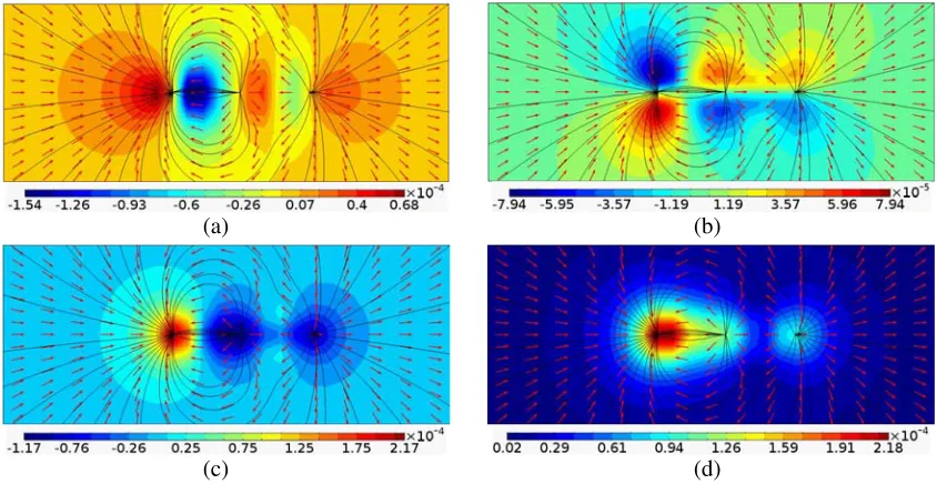
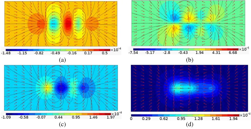
Assuming that the depth of seawater is 50 m and that the dive depth of submarine is 25 m, the electric field distributions of submarine under different conductivities are obtained through simulation. In order to analyze the influence of seawater conductivity on corrosion electric field, the plane (Z =−16 m) below the submarine was selected for observation. Figs. 4, 5 and 6 show the distributions of three components and modulus of corrosion electric field at conductivities of 2.5 S/m, 4 S/m and 5.2 S/m, respectively. The streamline and red arrow represent electric field lines and directions of X
andY components on the plane ofZ =−16 m, respectively. It can be seen that the surface distribution of electric fields under different conductivities have the same characteristics, but the amplitude becomes smaller with the increase of conductivity. The electric field distribution with the conductivity of 2.5 S/m is taken as an example to analyze the distribution characteristics. Electric field has a large change in the vicinity of submarine; furthermore, x-component, z-component and modulus are symmetrically distributed on both sides of the XOZ plane. However, y-component is anti-symmetrically distributed on the XOZ plane. Two positive current sources and a negative current source (the intersection of electric field lines) are present at the electric field plane. One of the positive sources represents corrosion current generated by damage, and the other positive source represents corrosion current generated by coating hull. Although Fig. 3(b) shows that anodic polarization current of coated carbon steel is very small, the coating area is much larger than the area of damage and propeller, so the current generated by coating hull cannot be ignored. The negative source indicates that corrosion current generated by damage and coating hull flows to propeller together.
In order to more intuitively analyze the distribution of underwater electric field, a path was selected under the submarine for observation, and the three components and modulus of electric field were
(b) (a)
(d) (c)
(b) (a)
(d) (c)
Figure 5. Electric field distribution of (a) x component, (b) y component, (c) z component and (d) modulus on theZ =−16 m plane when seawater conductivity is 4 S/m.
(b) (a)
(d) (c)
Figure 6. Electric field distribution of (a) x component, (b) y component, (c) z component and (d) modulus on theZ =−16 m plane when seawater conductivity is 5.2 S/m.
analyzed. Since submarine is symmetric about the XOZ plane and considering that the damage of coating symmetrically distributes on port and starboard, the transverse electric field component of Ey
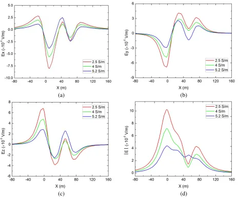
generated by corrosion current field on the keel is zero, so the path with the point (−80, 16, −16) m and point (160, 16, 16) m as endpoint is selected as the observation object. Fig. 7 shows the line distribution of three components and modulus of electric field. x-component has positive peak near x = −20 m and x= 40 m, respectively, and a negative peak near x= 10 m;y-component has a negative peak near
x = 0 m (propeller) and a positive peak near x = 28 m; the distribution of z-component is opposite to y-component, that is, there is a positive peak near x = 0 m (propeller) and a negative peak near
(b) (a)
(d) (c)
Figure 7. Electric field distribution of (a) x component, (b) y component, (c) z component and (d) modulus on the observation path when seawater conductivity is 2.5 S/m, 4 S/m and 5.2 S/m, respectively.
maximum value of electric field modulus is 1.02×10⁻⁴V/m. When conductivity increases to 4 S/m and 5.2 S/m, the maximum value of electric field modulus is reduced to 7.16×10⁻⁵V/m (30% decrease) and 4.37×10⁻⁵V/m (57% decrease), respectively. The influence of seawater conductivity on corrosion electric field mainly has the following two reasons. On the one hand, when conductivity increases, the current density in seawater increases if the potential difference of ship hull remains constant, but the magnitude of increase in conductivity is greater than in current density. It is known from Equation (15) that the electric field intensity is reduced. On the other hand, the oxygen concentration in seawater decreases when conductivity increases, and the ultimate diffusion current density of oxygen reduction is:
ilim=nF DO2CO2
l (16)
4.2. Comparison with Electric Dipole Model
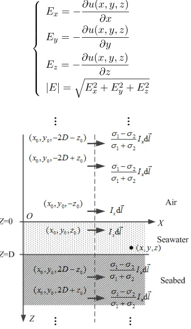
In order to verify the accuracy of BEM model in this paper, the simulation results are compared with the results of electric dipole model. The equivalent electric dipole model for solving the corrosion electric field of ship by mirror image method [7] is shown in Fig. 8. The figure shows the position and corresponding dipole moment of all dipole after the original dipole and mirror dipole are mirrored twice by the air-seawater and seawater-seabed interface. The potential that is generated by horizontal DC dipole Ixdllocated in seawater of (x0, y0, z0) at (x, y, z) is equivalent to the superposition of potential generated by the source and its numerous mirror dipoles formed through two interfaces at the field point. Therefore, the potential at field point (x, y, z) is expressed as:
u(x, y, z) =
∞
k=1
ηkIxdl(x−x0) 4πσ1r13k
+ η
kIxdl(x−x0)
4πσ1r23k
+ ∞ m=0
ηmIxdl(x−x0) 4πσ1r13m
+η
mIxdl(x−x0)
4πσ1r32m
(17) where ⎧ ⎪ ⎪ ⎨ ⎪ ⎪ ⎩
r1k= (x−x0)i+ (y−y0)j+ (z−2kD+z0)k
r2k= (x−x0)i+ (y−y0)j+ (z−2kD−z0)k
r1m= (x−x0)i+ (y−y0)j+ (z+ 2mD−z0)k
r2m= (x−x0)i+ (y−y0)j+ (z+ 2mD+z0)k
Dis the depth of seawater; η= σ1−σ2
σ1+σ2;σ1 andσ2are conductivities of seawater and seabed, respectively;
Ixd−→l is dipole moment of source; (x, y, z) is position of field point; and (x0, y0, z0) is position of source dipole. The electric field distribution in seawater is solved by Formula (18):
⎧ ⎪ ⎪ ⎪ ⎪ ⎪ ⎪ ⎪ ⎪ ⎪ ⎨ ⎪ ⎪ ⎪ ⎪ ⎪ ⎪ ⎪ ⎪ ⎪ ⎩
Ex =−∂u(x, y, z)
∂x Ey =−∂u(x, y, z∂y )
Ez =−∂u(x, y, z∂z )
|E|=
E2
x+Ey2+Ez2
(18)
(b) (a)
(d) (c)
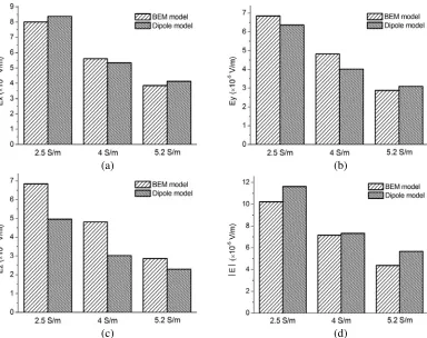
Figure 9. The maximum absolute values of (a) x-component, (b)y-component, (c)z-component and (d) modulus for BEM model and electric dipole model.
Consider that the depth of seawater is 50 m and that the source dipole is located at a depth of 25 m. The seawater conductivity is 2.5 S/m, 4 S/m and 5.2 S/m, respectively, and the seabed conductivity is 0.4 S/m. Fig. 9 shows a comparison of simulation results of the BEM model and the electric dipole model; moreover, Figs. 9(a), (b), (c) and (d) represent the maximum absolute values of x-component,
y-component,z-component and modulus, respectively. In the simulation results of the two models, the electric field values of x-component, y-component and modulus are relatively close, and the error is basically about 10%, which is within the acceptable error range. However, the error of z-component is obvious, and the errors of two methods reach 37.90%, 59.20% and 24.89% when the conductivities are 2.5 S/m, 4 S/m and 5.2 S/m, respectively. The reason for the obvious error of the two models on
z-component may be that the entire infinite space region was set to sea area without considering the influence of seabed on electric field in BEM model, while the three layers medium of air, seawater and seabed was considered in electric dipole model. Since seabed conductivity is much smaller than seawater conductivity, the presence of seabed weakens the z-component [10, 21]. Therefore, the z -component obtained by BEM model is larger than the z-component of electric dipole model, which is consistent with the simulation results.
The results obtained by boundary element method have high similarity in the maximum absolute values of electric field compared with the electric dipole model. Furthermore, the former has two obvious advantages. On the one hand, the simulation results of BEM can better reflect the distribution characteristics of corrosion electric field. Only the positive charge source at damage and the negative charge source at propeller are considered to constitute the electric dipole but not including positive charge source generated by coating hull in electric dipole model. However, the influence of the positive charge source on the distribution of corrosion electric field cannot be neglected, which has been discussed in Subsection 4.1. Moreover, the electric field plane distribution obtained by BEM (Fig. 4, Fig. 5 and Fig. 6) shows the existence of a positive charge source. Fig. 10 shows the distribution of electric field
Figure 10. The distribution of electric field x-component on the observation path obtained by BEM and electric dipole model when seawater conductivity is 4 S/m.
The result obtained by BEM reflects the influence of positive charge source generated by coating hull on electric field distribution. Furthermore, the peak of electric field moves about 9.5 m toward the bow due to the existence of positive charge source. On the other hand, the BEM is more convenient and concise. An important parameter called as electric dipole moment is indispensable when using electric dipole model to simulate the ship’s corrosion electric field distribution. It is mainly obtained through experience and literature; moreover, it will change significantly when the area and position of damage undergo changes (the area affects Ix, and the position affects d−→l ). At this time, it is difficult to accurately obtain the corresponding electric dipole moment that affects the calculation accuracy of corrosion electric field directly. However, it only simply alters the size and position of damage in physical model by BEM.
5. CONCLUSIONS
In this paper, the three-dimensional boundary element method is employed to simulate the corrosion electrostatic field distribution of ship, and the influence of seawater conductivity on corrosion electric field is studied. The electric field distribution is only slightly influenced by conductivity of seawater; however, the electric field intensity decreases as seawater conductivity increases, which can be explained by Equations (15) and (16). The simulation results of BEM model and electric dipole model were compared, and the error of x-component, y-component and modulus were about 10%. Since the influence of seabed was not considered in BEM model, the simulation result of z-component is too large compared to electric dipole model. The BEM modeling was proved to have validity for predicting the corrosion electric field distribution of submarine in marine environments. Moreover, it is a more convenient and concise modeling method that can better reflect the distribution characteristics of ship’s corrosion electric field than the electric dipole model. In future research, we intend to develop a seabed physical model in the BEM to simulate the influence of seabed on corrosion electric field, which is expected to reduce the error of electric field z-component.
ACKNOWLEDGMENT
This work is supported by the National Natural Science Foundation of China (Grant No. 41476153) and the author wishes to appreciate the technical support of COMSOL software company.
REFERENCES
2. Doose, J., “Numerical analysis of propeller-induced low-frequency modulations in underwater electric potential signatures of naval vessels in the context of corrosion protection systems,”Comsol Conference, 1–8, 2009.
3. Song, L. I., M. Shi, J. D. Luan, et al., “The feature extraction and detection for shaft-rate electric field of a ship,”Acta Armamentarii, 2015.
4. Holmes, J. J., “Application of models in the design of underwater electromagnetic signature reduction systems,”Naval Engineers Journal, Vol. 119, No. 4, 19–29, 2007.
5. Kumar, P. A., B. C. Mouli, and S. Ganesh, “Extraction of target parameters using underwater electric field analysis,”IEEE International Conference on Communication and Electronics Systems, 1–5, 2017.
6. Lu, J. J., R. Y. Yue, and F. Yu, “Monitoring and analysis of the marine underwater electric field of the typical shallow sea area,” International Conference on environment and Engineering Geophysics, 2012.
7. Li, K., “Electromagnetic fields in stratified media,” Advanced Topics in Science & Technology in China, Vol. 378, No. 2, 409–415, 2009.
8. Sampaio, E. E. S., “Primary electromagnetic field in the sea induced by a moving line of electric dipoles,” Wave Motion, Vol. 43, No. 2, 123–131, 2005.
9. Schaefer, D., J. Doose, and M. Pichlmaier, “Conversion of UEP signatures between different environmental conditions using shaft currents,” IEEE Journal of Oceanic Engineering, Vol. 41, No. 1, 105–111, 2016.
10. Schaefer, D., J. Doose, and M. Pichlmaier, “Comparability of UEP signatures measured under varying environmental conditions,”International Marine Electromagnetics Conference, 2013. 11. Kim, Y. S., S. K. Lee, and H. J. Chung, “Influence of a simulated deep sea condition on the cathodic
protection and electric field of an underwater vehicle,”Ocean Engineering, Vol. 148, 223–233, 2018. 12. Santos, W. J., J. A. F. Santiago, and J. C. F. Telles, “Optimal positioning of anodes and virtual sources in the design of cathodic protection systems using the method of fundamental solutions,”
Engineering Analysis with Boundary Elements, Vol. 46, 67–74, 2014.
13. Abootalebi, O., A. Kermanpur, and M. R. Shishesaz, “Optimizing the electrode position in sacrificial anode cathodic protection systems using boundary element method,”Corrosion Science, Vol. 52, 678–687, 2010.
14. Santos, W. J., J. A. F. Santiago, and J. C. F. Telles, “Using the Gaussian function to simulate constant potential anodes in multiobjective optimization of cathodic protection systems,”
Engineering Analysis with Boundary Elements, Vol. 73, 35–41, 2016.
15. Xing, S. H., Y. Li, and H. Q. Song, “Optimization the quantity, locations and output currents of anodes to improve cathodic protection effect of semi-submersible crane vessel,”Ocean Engineering, Vol. 113, 144–150, 2016.
16. Kim, Y. S., J. Kim, D. Choi, et al., “Optimizing the sacrificial anode cathodic protection of the rail canal structure in seawater using the boundary element method,” Engineering Analysis with Boundary Elements, Vol. 77, 36–48, 2017.
17. Lan, Z., X. Wang, and B. Hou, “Simulation of sacrificial anode protection for steel platform using boundary element method,”Engineering Analysis with Boundary Elements, Vol. 36, No. 5, 903–906, 2012.
18. Wu, J. H., S. H. Xing, and C. H. Liang, “The influence of electrode position and output current on the corrosion related electro-magnetic field of ship,”Advances in Engineering Software, Vol. 42, No. 10, 902–909, 2011.
19. Kim, Y. S., S. K. Lee, and J. G. Kim, “Influence of anode location and quantity for the reduction of underwater electric fields under cathodic protection,” Ocean Engineering, Vol. 163, 476–482, 2018. 20. Hack, H. P., “Atlas of polarization diagrams for naval materials in seawater,” 1995.
![Fig. 1 [19]. The uniform seawater medium is represented by Ω, and the boundary of the seawater domainis composed of S1, S2, S3a and S3c in the picture](https://thumb-us.123doks.com/thumbv2/123dok_us/1971323.1260182/2.612.189.433.449.619/uniform-seawater-represented-boundary-seawater-domainis-composed-picture.webp)