9 Form Follows Function: Reformulating Population Density Functions

Form Follows Function:

Reformulating Population Density

Functions

A simple isolated bit of evidence, however striking, is always open to doubt.Itis the accumulation of several different lines of evidence that is compelling. (Crick,

1990,p.37.)

9.

1 Cities as Population Density Functions

We could have written this book by beginning with existing theories of city size, shape and distribution and then gradually showing how fractal geometry could be used to reinterpret, generalize and extend the body of theory which geographers, economists and planners have been working with for the last hundred years. But instead we chose a different tack, intro-ducing fractal geometry first and tracing out its implications for how cities might be organized, before we embarked upon the ways in which our the-ory of the fractal city might link to the mainstream of urban studies. With-out our having reviewed the multitude of urban theories in other than cur-sory terms, it is already clear that fractal geometry has appealing properties with respect to cities in ideas concerning space-filling, self-similarity and density. In fact as Crick (1990) implies above, although these lines of evi-dence for a fractal theory of cities are highly suggestive, they become com-pelling when it is realized that much of what has been developed in the mainstream is entirely consistent with fractal geometry.

Social forces between populations in space were described explicitly by Carey in the' mid-19th century using gravitational analogies, while the notion that the density of economic activity declines with increasing dis-tance from its market is implicit in the work of von Thunen, circa 1830 (Hall, 1966). In the study of population densities, it is now just over 100 years since Bleicher (1892) wrote: "The rapid decrease in population density with distance from the center is highly characteristic of an old city such as ours" (Edmonston, 1975; Mogridge, 1984).

However another 50 years were to elapse before these observations were associated with specific mathematical functions. There is some evidence that such functions were being used in the 1940s(Ajo, 1944), but it is Colin Clark (1951, 1967) who is accredited with the first use of the negative exponential function as the basic model for population densities. Since then, many variants of this model have been developed. The negative exponential density function is consistent with the theories of strict utility-maximizing associated with urban economic theory (Beckmann, 1969; Muth, 1969), while the development of operational urban models based on entropy-max-imizing (Wilson, 1970) and discrete choice theory (Anas, 1982) which we introduced, albeit briefly, in Chapter 4, make widespread use of such func-tions. Although early analogies with gravitational models based on the inverse square function of distance formed the foundations of social physics in the 1940s and 1950s (Stewart, 1941, 1950), these power functions were quickly replaced with the negative exponential in the 1960s and 1970s due to the analytical convenience of such functions in problems of economic and statistical optimization, as well as to the elegance of the mathematical forms produced.

These developments, however, appear to have lost sight of the fact that the density and flow of economic activity across space must be fundamen-tally constrained and thus determined by the geometrical properties of their physical systems. It is clear that there is much misunderstanding of these issues, as Stewart (1950) was never slow to point out. Others such as Col-eman (1964) who have considered the foundations of social physics have reinforced the point that power functions in their inverse form are the most obvious ones which embody the physical properties of the correct systems of interest (Batty and March, 1976). But such views have never attracted much attention and have remained apart from the mainstream of urban analysis during the last three decades. What a fractal theory of cities offers is a coherent approach to these earlier traditions.

form of the systems they describe. In short, their parameters can be associ-ated with the extent to which their systems exploit the space in which they exist, the fractal dimension being directly associated with these parameters and with the extent to which the form fills the space available. The form or morphology of the system is no longer a prerequisite to models of its functioning, but a consequence of the way the system works in space. In this sense then, we will be dealing with systems in which 'form follows function'.

This chapter will attempt to weave several diverse themes together. Once again, we will note the work on urban allometry in which the size of the urban system is related to the space it occupies (Stewart and Warntz, 1958; Dutton, 1973), we will show how densities based on power functions arise as a natural consequence of such allometry, and we will cast our argument in terms of the new physics of fractional dimension (Davies, 1989) which uses the empirical ideas of Chapter 7 explicitly and the DLA and DBM models implicitly. We will first examine the properties of the negative exponential and inverse power functions, showing that the inverse power function has certain properties for describing urban population densities which have hitherto been overlooked. These properties can be easily exploited through scaling laws appropriate to urban systems, and accord-ingly, we show how urban form follows quite naturally from such func-tional descriptions. In this sense, we are also able to show that the density parameters associated with these functions are directly related to the frac-tional or fractal dimensions of the space within which these city systems exist.

9.2 Exponential Functions of Urban Density

Clark's (1951) original model assumes that population density p(r) at dis-tance rfrom the center of the city (r=0) declines monotonically according to the following negative exponential

p(r)=K exp(-Ar), (9.1)

whereKis a constant of proportionality which is equal to the central density

p(O) and Ais a rate at which the effect of distance attenuates. Note that in this chapter we will use A for the density parameter of the negative exponential and Q'. for the inverse power function. ~ will be used as pre-viously as a general regression parameter of various scaling relations from which the fractal dimension D can be derived. As previously, we will use the variablerto indicate a variable distance from the CBD, whereas Rwill be used to define the accumulation of distance which is an integral ofr up to the radiusR. r should not be confused with its use as a measure of scale in earlier chapters, but its use should be obvious from the context.

Clark's (1951) paper was wide-ranging, idiosyncratic and brilliant; he not only fitted the log transform of equation (9.1) to over 20 cities using linear regression but also speculated on how the parameter Achanged through time, thus charting from the beginning, the direction for all subsequent empirical work on urban density functions. It is still not clear why Clark chose the negative exponential function for he was unaware of Ajo's (1944) doctoral dissertation in which a negative exponential function was used to model traffic flow in the Finnish city of Tampere.Itis likely, however, that this function was chosen because it was popular in mathematical economics in models of capital depreciation and the like of which Clark was prob-ably aware.

In the parallel development of social physics, inverse power functions of distance were being widely exploited in gravitational models of traffic flow and in rank-size relations. But there were no attempts to collapse such gravitational models to models of population density until the early 1960s when Smeed (1961, 1963) suggested a suitable such model might be based on

p(r)= KrCY., (9.2)

drowned out any further attempts to model population densities by any-thing other than negative exponential functions.

So far, the body of work concerned with population density models is almost exclusively based on the negative exponential function or its gen-eralization. As Zielinski (1979) points out, attempts at demonstrating the precedence of one function over another in this field are quite inconclusive and in the absence of further empirical evidence, theoretical considerations suggest the negative exponential function as being superior. There have been some dissenting voices. Smeed's (1961) work has been noted, and Blu-menfeld (1972) (summarized in Vaughan, 1987) and Saviranta (1973) have both argued for inverse power functions of density. However, there has been more work at seeking a generalized function such as the gamma whose typical form is

per)=KrQ _{exp(-X-r), (9.3)}

where the parametersK, ex andX- fulfill the same roles as in equations (9.1) and (9.2). Tanner (1961), March (1971) and Angel and Hyman (1976) have suggested that functions such as(9.3) are general enough to encompass the various debates about one functional form or the other. Finally, it is worth noting that Parr (1985a, b) amongst others has suggested that the negative exponential function is more appropriate for describing density in the urban area itself, while the inverse power function is more appropriate to the urban fringe and hinterland. In later work, Parr and his colleagues have argued that the most appropriate generalized function of density is the log-normal (Parr, O'Neill and Nairn, 1988: Parr and O'Neill, 1989); this relates to processes which generate such functions, which in turn relate to the use of such functions in fractal geometry.

The most obvious interpretation of the parameter X- in the negative exponential can be made by taking the first derivative of equation (9.1). Then

dp(r)

dr

=-X-Kexp(-X-r)

=-X-p(r),

and thus

(9.4)

(9.5)

dp(r) per) =-X-dr,

which implies thatX- is the percentage change in density for a small change in distance dr. In this sense then, the parameter plays a crucial role in the

calculation of elasticities in the fully-fledged urban economic theory of the housing market which gives rise to this function (Muth, 1969).

r is the line of distance and 8 is the angular variation, both about the center. Note that we will use the terms one-directional and two-directional only in those contexts whereitis necessary to draw distinctions between direc-tion and dimension. In all other contexts, the term dimension will suffice for both (Batty and Sikdar, 1982).

We will first examine the one-directional function. Note that in the sequel, we will normalize the density over its space to sum to unity. Then

J:b

p(r) dr

=

J:b

K exp(-Ar)dr

=

1, (9.6)

where Rb marks the distance to the boundary of the spatial system. Evaluat-ing equation (9.6) gives the constantK as

K

=

1-

e~(-ARb)'

(9.7)

and therefore the density becomes

A exp(-Ar)

p(r)=1 _ exp(-ARbr (9.8)

Clearly when Rb-+ 00, the value ofK = A. The cumulative distribution of

p(r), N(R), is given as

N(R)

=

J:

p(r) dr

1 - exp(-AR)

=1 ( \R )= 1 - exp(-AR). (9.9)

- exp -I\. b

However, it is the mean density in the city which is of most interest, and this is defined as

C(Rb ) =

J:b

p(r) r dr

1 Rb exp(-ARb) (9.10)

=

x: -

_{1 - exp(-ARb)·}

In equation (9.10), ifRb-+ 00, then C(oo)

=

l/A and the interpretation of A

is as an inverse measure of the mean density, thus controlling the spread of the function in the linear direction.

The same type of analysis as presented in equations (9.6) to (9.10) can be developed for the two-directional model which we stated earlier in polar coordinates as p(r, 8). The density function is now given as

p(r,6)

=

K exp(-Ar),

and its normalization as

J:n J:b

p(r, 0)r dOdr

=

21TK

J:b

exp(-Ar)r dr

=

l.

The normalizing constantK can be evaluated as A,z

K =

-27T {I - (1+_{ARb) exp(-ARb)}"}

(9.11)

(9.12)

(9.14)

(9.15)

From equation (9.13) when Rb -.00,thenK= X2/27'1. The cumulative

distri-bution functionN(R) is

N(R) = 1 - (1+XR) exp(-XR)

1 - (1+XRb) exp(-XRb)

= 1 - (1+XR) exp(-XR).

and the mean density

C(Rb )

=

r

f:

b

p(r,0)t"-dOdr

2 XR~exp(-XRb)

=

x: -

1 - (1+_{XRb) exp(-XRb)'}

As Rb -.00, C(oo) = 2/X, thus implying that X is also an inverse measure of

mean density controlling the spread of the function over the two directions of space (Batty,1974).

When the boundary distance Rb- ' 0 0 ,XC=1for the one-directional

func-tion and XC = 2 for the two-directional. In this context, it is possible to associate direction with dimension, the dimension of the spatial system entering the calculation of the parameter X directly. To anticipate an argu-ment of a later section, the spread of developargu-ment is unlikely to be over the entire two-dimensional space, but it is likely to be spread over more area than the one-dimensional line. Therefore it is likely that 1

<

XC

<

2, and thus the value of XC is a measure of the extent to which the density fills two-dimensional space, if and only if Rb defines a good approximation to the spread across space of the density function. We will now develop the same analysis as contained in equations(9.6)to(9.10)and(9.11)to(9.15)

for the inverse power function.

9.3 Power Functions of Urban Density

An immediate interpretation of the parametera in the scaling function in equation (9.2) is provided by its first derivative

dp(r) a

- - = - - p(r)

=

-aK-a-l,

dr r

which can be written as

(9.16)

(9.17)

dP(r)/dr --ex

p(r) r - ,

where ex is clearly an elasticity, the ratio of the percentage change in density dp(r)/p(r) to the percentage change in distancedr/r.Inequations(9.16)and

(9.17), a has a more precise interpretation than the negative exponential parameter X in equations (9.4) and (9.5), but its role is similar.

(9.20) model and then repeat the analysis for two. The normalization of equation (9.2) is given by

J:b

p(r) dr

=

Kr"dr

=

1. (9.18)

The integral in equation (9.18) cannot be evaluated when r = 0, for the function p(O) is infinite at this value. This has been one of the main reasons for researchers preferring the negative exponential. However, the problem can easily be dealt with by translating the origin of system to a value ofr

> 0,r

=

1 being the obvious lower limit. Some have argued that population density is not defined at the center of the city in any case or that population density at a point is meaningless although neither of these assumptions are necessary to the shift of the origin which is arbitrary. Evaluating the integral in equation (9.18) from

r

=

1 to

r

=

Rb gives

I-a

K = (9.19)

R~-a-1

and

(r)= (1 - a)ra•

p R~-a- 1

As Zielinski (1979) points out, the normalization in equations (9.19) and (9.20) is still "analytically awkward", and further indefinite integrals are impossible to evaluate. With a little simplification, however, it is possible to proceed. Firstifthe boundary of the systemr =Rb is much greater than r= 1, then it is possible to ignore the lower limit; second if it is assumed that a lies between 0 and 1, then equation (9.20) will always act as an inverse power function. Moreover, ifa 2::: 1, then the function breaks down, and is no longer meaningful as a model of population density. Thus the use of equation (9.20) implies that there are tight bounds on the value ofa.

With these assumptions, the cumulative density function can be written as

N(R)

=

r

p(r) dr

R(I-a)

=- -

=

R(I-a). RbI-a)

Finally the mean density C(Rb ) is evaluated as

C(Rb ) =

t

p(r) rdr

I-a =-2- Rb.

- a

(9.21)

(9.22)

and this shows that the parameter a depends directly upon the value of the system boundary Rb • From equation (9.22), the parameter a can be

computed as

2C(Rb ) - Rb a = C(R_b) - R

bI

but this is still an approxim~tionwhose relevance cannot be judged in advance of any particular application. However, equation (9.23) does pro-vide some bounds on the value of <x,namely that asRb

>

C(Rb ), then ex:5

1.The analysis for the two-directional model follows directly. The normaliz-ation is given as

f:

W

f~

p(r, e)

r

dr de

=

2-rrK

fb

r "

r

dr

=

1,

from whichK can be evaluated as

2-ex

K -- 27i"(R~-a - 1>"

Assuming that Rb ~ I, then the density p(r, e) becomes

( ) (2 - ex)

,a

pr,e =

-27i"R~-a

and the cumulative density is

f

2'lT fR

N(R)= 0 1 p(r,e)r drde

The mean density C(Rb ) is now evaluated as

(9.24)

(9.25)

(9.26)

(9.27)

(9.28)

(9.29)

C(Rb ) =

rr

p(r, e)

r

dr de

2-ex = - - Rb ,

3-ex

and this has the same structure as equation (9.22) for the one-directional model. Itis possible to compute exfrom equation (9.28) as

3C(R_{b ) -} 2Rb

ex= ,

C(Rb ) - Rb

and from this, it is clear that ex is unlikely to be greater than 2. The real significance of equations (9.23) and (9.29) however is that they show that the parameter exof the inverse power model is critically dependent on the boundary of the system Rb , and in certain empirical contexts, it will be

possible to estimate exfrom these equations.

Although the differences between the two functions elaborated through equations (9.4) to (9.15) and (9.16) to (9.29) are substantial in mathematical terms, in practice both have been shown to fit empirical data equally well (or equally badly). In this section we will seek to demonstrate this. In Figure 9.1, one-dimensional negative exponential and inverse power functions from equations (9.8) and (9.20) respectively are plotted up to a regional boundary Rb = 50 units of distance. The parameters X. and ex have been

0.015

p(r)-r··

-.:.. Q.

0.003

/ p (r)-exp(-"')

t

o-n--:-,--,----,---r-+-I

--r---.---01 :

t

:

4.011 33.722

C (Rb)=20

Figure 9.1. Acomparison of the negative exponential and inverse power functions.

a = 0.349 have been estimated which give simulated mean densities for both functions within 0.01%of the predetermined mean. Before we explore these functions further, it is worth noting for the inverse power function thatifequation (9.23) is used to predicta,which is based on the assumption that the lower limit ofr is 1, then the value of this parameter is 0.333 which is within 5% of the computed value.

No simple solution for the parameter Aexists for the negative exponential model. A first approximation to A based on l/C gives 0.05 while the use

of the two-dimensional equation2/Cgives 0.1. The actual computed value is half the one-dimensional approximation, thus implying that the negative exponential over the given range fromr =0 tor=50 provides only a partial approximation to its overall spread. This can be easily seen in Figure 9.1 where the inverse power function is much steeper in the area of its origin compared to the negative exponential which has a more gradual slope over the same distance to which it is applied.Amore direct comparison of these functions can be made over their intermediate ranges where, from Figure 9.1, it is clear that the functions are similar. These functions will cross at r

=

4.011 andr

=

33.722, which are solutions to the equation of the two model functions {A exp(-Ar)/[l - exp(-ARb )]} = {(I - a)r1-a/Rl,-a}. It is between

these two values that the functions are similar.

variation in density, the inverse power being used to model peripheral vari-ation (Parr, 1985a).

One of the main reasons for the popularity of the negative exponential function in population density models relates to its elegant properties. In

fact, as we have shown above, these properties can only be fully exploited when it is assumed that the regional boundary distance is infinite; in short, this is only the case when the infinite boundary provides a good approxi-mation to the observed density field. In the given hypothetical example as well as in the applications to Seoul which follow, this is clearly not the case and it is the inverse power model which yields more tractable equations which can be exploited in rapid estimation. Furthermore, although the negative exponential emerges 'naturally' from entropy-maximizing, this is due to the constraint on total travel distance adopted. There is in fact con-siderable evidence to suggest that distance perception is logarithmic, this being the basis of the Weber-Fechner law in psychology.Ifthe logarithmic constraint on travel distance is used, then it is easy to show that the inverse power function is the appropriate derivation using entropy-maximizing. On balance, it is our view that both functions are useful in different contexts. Moreover, we should not ignore Zielinski's (1980) comment: "Since both (functions) can give practically identical fits to data, what criteria should be adopted to prefer one to the other? In this case the pragmatist must take the back seat to the theoretician. And theoreticians must endeavor to prove their assumptions". This we will attempt to do in the following sections.

9.4 Urban Allometry, Density and Dimension

Inthe growth and evolution of natural systems, there has been considerable research into the ways various features of such 'systems scale with increas-ing size, the study of relative sizes beincreas-ing allometry (Gould, 1966). We briefly alluded to this line of research iRChapters 2, 6 and 7, but here we provide a more complete summary in preparation for this and the next chapter. Allometric relationships relate the size of an object to a familiar yardstick such as length. For example, taking a measure of size in terms of the dimen-sion of a systemE, in Euclidean geometry we can define points where E

=

0, lines whereE

=

I, planes where E

=

2 and so on.Ifwe take the yardstick as a measure of length in one dimension, that isRsay, then objects which scale as a point vary as RO, as length itselfR1

, as the planeR2 and so on, in general the scaling relation beingRE

•Ifthe size of the object in question

is expected to scale asRE

, we refer to this as isometric scaling.Ifthe object

scales as RD _withD

_<

_{E, then this is called negative allometry and if D}

_>

E, this is positive allometry.

In its most basic form, population density can be considered as the sca-ling between populationN(R) and areaA(R), however defined, whereRis some measure of the linear dimension of the space. Then the key scaling relation betweenN(R) and A(R) can be written as

Froma prioriconsiderations, we can argue that the value of the parameter <I>indicates how population fills the two-dimensional space available to it. If <I>

>

1, then the population fills more than the two dimensions of the

space, while if <I>

<

1, population is filling less than its available space. There have been several studies of this allometric relation over different sizes of cities based on the general assumption that as cities grow into the third dimension, then equation (9.30) should exhibit positive allometry. This is borne out in the work of Stewart (1947) and Stewart and Warntz (1958) where they show that <I> = 4/3 for British and American cities with 1951 data. With Swedish data for 1966, Nordbeck (1971) concludes that <I>

= 1.506 which is a little larger than 3/2 which would be the value if cities filled the three dimensions available to their development. More recently, Jones (1975) following work by Best, Jones and Rogers (1974), has derived

<I>as 1.193 for cities in England and Wales from the 1971 Population Census, and Craig and Haskey (1978) who reworked these data concluded that <I>

has remained approximately stable since 1951 with a value between 1.41 and 1.45. However, Woldenberg (1973) using data for American cities has shown that <I> varies from around 0.8 to 1.2 depending upon the data set

used.

All these studies refer to data sets based on wide ranges of city size. In the intra-urban case, where population densities decline with increasing distance from the center, equation (9.30) will show negative allometry. First we will replace the measure of area in equation (9.30) with the yardstick of length R which enables us to link this analysis to population density functions introduced above. Then equation (9.30) can now be written

N(R)='YA<l>

='Y('Ti'R2)<l> = <pRD, (9.31)

where we have assumed that the distance associated with the area is given as R

=

-VA,

and 'Y and <p are constants of proportionality. From equation

(9.31) it is clear that D = 2<1> and if <I>

<

1, then D

<

2. Takayasu (1989) refers to D as the 'effective dimension', but to anticipate our argument, this of course is the fractal dimension. As in the two previous chapters, the value of D is thus a measure of the extent to which the city fills its two-dimensional area.

Without anticipating the value of D for any particular city, we can now present the equation for population density in terms of the scaling relation based on the yardstick of length R and explicitly containing the parameter D. From equations (9.30) and (9.31), we will write the density as in equa-tions (2.33) and (7.9)

p(R)

=

~~~i ~

A(R)<l>-l, (9.32)

and from this it is clear that if population is isometric with area and <I> = 1, then p(R) is constant. For population density to decline with increasing distance from the center, then the exponent in equation (9.32) must be less than 0, that is<I> - 1

<

1, while it is most unlikely that<I> would be greater

(9.33)

(9.34) and for the density to decline with distance, it is clear that the fractal dimen-sion D should be less than 2, implying that the city will not fill the two-dimensional space available.

The real value of this analysis is in revealing how density should be defined. Casual observation should suggest whether the city is filling two or three dimensions.Ifthe city fills less than the plane, then the appropriate space on which to compute density is the plane; thus the definition of area as A(R) = 'Ti'R2 _{in equation (9.32) is correct and the value of D will be less} than 2. However, if the city is filling three dimensions of space then the appropriate normalization by area would be A(R)= 'Ti'R3, the volume, and then the value of D would probably be greater than 2 but less than 3. In this case, the more general form of density equation in (7.18) would be appropriate. In fact, in all studies of density to date (of which the authors are aware), the implicit assumption is that cities fill the plane, not the vol-ume, thus suggesting that the argument made by Nordbeck (1971) amongst others that cities fill the third dimension is spurious.

The other important conclusion from this analysis is that the measure of area to be used represents the space within which the city grows, its field, not the more restricted area which is associated with its built-up form; in fact most studies of density based on the population and area of Census tracts treat the area of the field, although in some studies which use built-up area, the parameters derived cannot be compared with those here. What is certain, however, is that in most studies of population density to date, researchers have paid very little attention to the definition of area, thus throwing into question the validity of the parameter values estimated, at least in terms of the sorts of theory invoked here. Comparisons between different studies are therefore difficult to make.

9.5 The Basic Scaling Relations Revisited

We are now in a position to relate the density equations stated earlier in terms of the inverse power functions, to those derived from urban allometry. We will use the two-directional function given in equation (9.26). Equating this to the density in equation (9.33), we will integrate over 8. Then

p(R)=

I:w

p(R, 0) dO

=

K'R~

=

~D-2,

and if the equation holds, then D - 2

=-

(Xor(X

=

2 - D. As D is a measure

of the extent to which space is filled, then it is expected to be less than 2, and thus(Xis its complement, a measure of the extent to which the available

(9.36)

N(R)=K"R2-a=(f>RD. (9.35)

Equations (9.34) and (9.35) suggest a coherent and useful coincidence between the fractal dimension D and the parameter of the associated inverse power function of population density; that is, that the two dimen~ sions of the associated space can be divided into a space-filling component D and a non-space-filling componenta which sum to the Euclidean dimen-sion E of the space within which the city exists, in short, that E

=

D +a

=

2. We have already defined three scaling relations, namely the population-area relation in equation (9.30), the population-radius relation in equations (9.31) and (9.35), and the density relation in equations (9.33) and (9.34). We will add to these a fourth relation, based on the first derivative of the cumulative population-radius relation in equation (9.35). This relation, referred to as the incremental population-radius equation, is derived as

n(R)=

d~1R)

=hRD-l=hRTI.

h is a constant of proportionality and TI is the scaling parameter. We now

have four scaling relations; three of these which relate the cumulative popu-lationN(R), the incremental population n(R), and the density p(R) to the radius R and based on equations (9.31), (9.36) and (9.33), are those used in Chapters 7 and 8 to describe the distribution of particles in the DLA and DBM simulations. These will be used here in the empirical analysis of den-sity in Seoul, but note that the alternate denden-sity variable Q(R) which was used in Chapters 7 and 8 and defined previously in equation (7.26) is not used. The fourth relation is the classic allometric equation which relates

N(R) to A(R) as in equation (9.30).

Before we broach the question of estimation, we must make clear the fact that we expect the value of the fractal dimension estimated from the Seoul data to be similar to that of the DLA simulations, that is D= 1.7, as implied in many of the estimates given earlier in Table 7.1. Thus the value of the density parameter would be around -0.3, that is a = D - 2. Earlier we speculated that in the case of the negative exponential density function, the dimension of the system would fall between 1

<

hC

<

2 from arguments relating to the mean density in one- and two-dimensional systems. We can now speculate that X.C = 1.7, a result which has already been borne out in work by one of the authors almost 20 years ago (Batty, 1976). Similar relations are not obvious for the inverse power function, although D and

a are immediate results of their estimation and further insights must await further research. To provide some sense of closure to this theoretical section and to progress the research to applications, methods of estimating equa-tions (9.31), (9.36), (9.33) and (9.30) in that order will now be discussed.

9.6 Methods of Parameter Estimation

and choosing appropriate estimation methods. We will deal with these issues in turn. Researchers fitting population density models have either dealt with the data in their raw form by Census tracts or have aggregated the data into concentric rings. The latter method produces better fits and hence more reliable estimates because local variations in the data are reduced, but the use of one or the other data set ultimately depends upon the purpose for which the analysis is undertaken. Here we will employ both, but we consider that the method of concentric rings is likely to give much 'truer' estimates of the values of the parameters D and a which is of most interest to the analysis performed here. In fact, this was the method which we used to organize the data in Chapters 7 and 8 for comparing the theoretical simulations with Taunton and Cardiff. A related issue involves the way the data are aggregated over distance and whether relationships are fitted in their cumulative or incremental form. Cumulative relations are bound to give better fits and this will be our emphasis although we will also examine some incremental estimates. In this sense then, we will follow the practice of Bussiere(1972) and Bussiere and Stovall (1981),rather than the traditional treatment used by Clark (1951).

The first method of estimation we will use and one that will act as our baseline, involves taking logarithmic transformations of equations (9.31), (9.36), (9.33) and (9.30) and estimating their parameters using linear regression. The four relations can now be summarized in discrete form as

log Ni=al +~l logRi , (9.37)

logni=a2+~2logRi, (9.38)

logPi=a3+~3logRi, (9.39)

log Ni=a4+~410gAi' (9.40)

Note first that the intercepts or constant terms all a2' a3 and a4 are not directly related to the parameter a of the inverse power function but are so defined to make them consistent with their usage in Chapters 7 and 8 through equations (7.49). Throughout the analysis, distances are ordered so that Ri

<

Ri+l

<

Ri+2, the cumulative populations are given as Ni= 'Sjnj'

(j= I, ...,i),the areas for each cumulative ring asAi='TTR~,the actual area of each ring as ai

=

Ai - Ai-I, (i > 0 and Ao

=

0), and the density Pi

=

nJai'

We also need to be clear about the various parameter estimates in these equations and the look-up table reproduced as Table9.1 shows the

conver-Table 9.1. Relationships between the parameters

Equation Intercept Slope Dimension Density

numberl _{parameter parameter D coefficient(X}

9.37 (9.31) (Xl = log'P ~l = D ~l 2 - ~l

9.38 (9.36) (X2= log h ~2 =1) 1+~2 1 - ~2

9.39 (9.33) (X3 = log~ ~3= D - 2 2+~3 ~3

9.40 (9.30) (X4= log 'Y ~4 = <l> 2~4 2(1 - ~4)

1 The first equation number in each row is the number of the log transform of the second

sion between these parameters, the dimension D and the coefficient a.. In the sequel, all estimates are given to three decimal places.

There are several other methods of estimation which we consider less reliable than log-linear regression. Mills (1970), Mills and Tan (1980), and Weiss (1961) all use methods which involve only two values of density or population given at two different points within the city. For example,ifthe density p(R) or the cumulative populationN(R) are known at, say, distances

Rand Rb , then using equations (9.26) or (9.27) in the two-dimensional case,

the constant and scaling parameters can be found from the solution of two equations in two unknowns using the Newton-Raphson method (Batty, 1976). There is little work on how reliable these types of estimates are in comparison with those from regression, but we consider that such methods are really only appropriate when no more than two observations are avail-able.

There are, however, two other methods which we will use, the first of which was introduced in Chapters 7 and 8 and which can only be usedif population data are available on a very fine lattice. Where each occupied lattice point is the location of a single equal-sized household, then a good approximation to the density in equation (9.33) is p(R) - RD-2 where the

constant of proportionality is approximately equal to unity. Then for any distance R from the center, D can be calculated from a log transform of this equation, given earlier in equation (8.13) which is restated as

(8.13)

In earlier chapters we called the graph ofD(R) against R the 'signature' of the density function. In the vicinity of its origin,D(R) can fluctuate wildly, butit soon settles down to a characteristic value (D{R) = 1.7 for the case of a DLA cluster). At the edge of the cluster, the value of the dimension is also umeliable because this is the area where the city is likely to be developing most rapidly. Thus the best value of the dimension will be given at the distance value of the mean density, that is at D{C(Rb )}.We have not

yet said anything about the data in the applications which follow, but two of the four data sets we will use are based on a crude approximation to the shape of the city using lattice point data which reveals the morphology of the city in question. This will become clear in the sequel.

The last method is well-known in that it is based on deriving the density and population model by entropy-maximizing. Formulating the model in terms of the location of populationnjin individual zones i, the model can be stated as

(9041)

or

- 2:

nj

C= -R·

N ' j

- ~ nj

Clog

=

L.J N log Rj • j

(9.42)

(9.43)

Strictly speaking, equation (9.41) is associated with constraint equation (9.43) not (9.42); that is, equation (9.41) is derived by maximizing entropy subject to equation (9.43), thus leading to the derivation of the inverse power function (Wilson, 1970). In fact, we will fit equation (9.41) by separ-ately solving for both equation (9.42) and (9.43), thus giving two estimates of'Yl (and thence of D anda through Table 9.1). We will not concern our-selves any further with entropy-maximizing except to point out that there is a strong relationship between entropy, information and fractal dimension which finds its clearest expression in the derivation of power functions such as thos~treated here (Batty and Sikdar, 1982; Takayasu, 1989).

9.7 Applications to Large Cities: the Seoul

Data Base

Seoul was selected for our empirical work because the negative exponential model has already been fitted to its population density, thus giving us the opportunity of making some casual comparisons to the inverse power den-sity models which we will estimate here (Kim, 1985). We also had access to reasonable population data for the city at three dates 1970, 1977 and 1982 from which we selected the 1982 data for our applications. Moreover, Seoul is a rapidly growing city, its population increasing from around 5.5 million in 1970 to almost nine million in 1982, and we consider that cities such as this one where rapid growth has taken place under few market imperfec-tions to be ideal testing ground for the ideas introduced here. The basic set of zones for the 1982 population data are shown in Figure 9.2(a) which are aggregations of Census tract data. In the analysis, the center of the city was found using centrographic analysis on the 1982 data (Kim, 1985). Distances to all other zones were then defined as crow-fly distances from this center to each individual zone centroid. From this original data set, the zones are ranked according to distance from the center and these are aggregated in the given order for estimating three of the four scaling relations.

(a)

(b)

Zonal System

Full Morphology

(c)

(d)

Zonal Morphology

Reduced Morphology

01-1--'----r-',---3.>,'OKms

o 2'0 Mis

Figure 9.2. Zonal and lattice systems for the four data sets.

detailed morphology of the city. In short, although each lattice point is assumed to have an identical population density, when aggregated for pur-poses of analysis into concentric rings say, then the variable density of population will be detected. This is clearly not the case here where the lattice is far too coarse; for it to pick up the kind of variation needed, the spacing should be as fine as 10 m x 10 m. Our gross approximation here is thus illustrative rather than definitive, and although it does pick up the morphology and variable density at a crude scale, the results of using this data set must be interpreted with caution. The coding is shown in Figure 9.2(b).

which produces the third, noting that the periphery of the city is excluded from the original urban morphology shown in Figure 9.2(b) due to the fact that population data is not available for these outer areas. The fourth and last data set is similar to the second except for the peripheral areas which have been excluded. This is simply formed by overlaying the first data set on the second, excluding the peripheral areas, thus forming a reduced morphology based on lattice spacing. This is shown in Figure 9.2(d).

For the second, third and fourth data sets which are all based in some way on the lattice morphology, concentric rings can be easily defined at increasing units of equal distance around the center.Inthese cases, we have divided the greatest radial distance to the edge of the city into 25 equal units on which we have arranged 25 concentric rings. The populations and related variables for each ring have then been derived by counting the num-ber of lattice units (and their populations in the case of the third data set) which fall into each ring.Insubsequent analysis, we will refer to these four data sets as follows; the first data set based on the zones shown in Figure 9.2(a) is called the Zonal System, the second in Figure 9.2(b) the Full Mor-phology, the third in Figure 9.2(c) the Zonal MorMor-phology, and the fourth in Figure 9.2(d) the Reduced Morphology.

It is also important to be clear about which estimation method is to be applied to which data set at this stage. All four scaling relations in equations (9.31), (9.36), (9.33) and (9.30) will be fitted to all four data sets using the logarithmic transformations given in equations (9.37) to (9.40). This will represent our set of baseline estimates for we consider this type of esti-mation as providing us with the most comprehensive set of estimates. This will generate four estimates of the dimension D and the density parameter a for each of the data sets. The estimates based on solving the entropy-maximizing constraint equations in (9.42) and (9.43) will also be applied to each of the four data sets. This will provide us with two sets of parameters D and a derived fromTJ,one for each solution of the appropriate constraint equation. Finally, the method of calculating D (and hence a) from the signa-ture given in equation (8.13) is only valid for the Full and Reduced Mor-phology data sets, the second and fourth, because this requires that the data be based on equally dense lattice points. This concludes our survey of the data and we will now embark on presenting the baseline estimates.

9.8 The Density Model Estimates

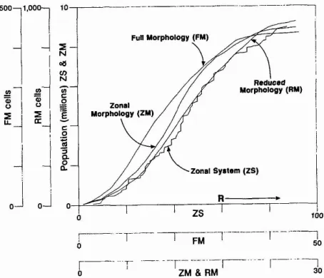
Throughout the process of fitting the baseline equations in (9.37) to (9.40) to the four data sets, the analysis was aided by frequent graphical interpret-ations of the base data, model predictions and residuals. To provide some sense of the similarities between the data sets, we have plotted the cumulat-ive population {Ni } against the radius {Ri } as given in equation (9.37). The

exten---~

\

!

i

I

!

I

I

--¥~--.----,---.----__r--~

100

r--- --

r---

--/"""---l--- -r-- ---l

o ~ w

r - - - T - ---T---r---1---1

o m&~ ~

Figure 9.3. Cumulative population profiles for the four data sets.

sive examples in Bussiere and Stovall, 1981). Using Figure 9.3,ifa detailed analysis is made of the variation in density and population in the vicinity of the origin and at the edge of the city, it is clear that density is volatile and shows no characteristic trend in these areas. Population density is notoriously difficult to model near the center of the city, while at the edge, the city is growing at its fastest rate, and the density is nowhere close to the density which will ultimately prevail.

The models therefore should not be applied in these areas; at the center whatever function is used is likely to be inappropriate, while at the edge, densities are likely to be too low, and thus the function will underpredict these. We will use these characteristics to exclude certain observations from our data set in the results presented below as we did with the simulation results and the empirical data pertaining to Taunton and Cardiff in Chap-ters 7 and 8. This is a particularly important issue in modeling population density, for we must assume that wherever the density function applies, the -city must be in equilibrium. In previous work, this issue has been entirely ignored for most research has not been cast into an appropriate dynamic framework which indicates that densities in the areas of the origin and periphery of a growing city are likely to be subject to rapid change. The theory of the growing city which we have alluded to here based on DLA simulations provides a strong rationale for systematically excluding these areas from our estimation and accordingly, we will proceed by doing so.

Table 9.2.

Dimensions associated with the Zonal System data

Number of Population- Incremental Population

Population-zones radius population density area

(9.37) (9.38) (9.39) (9.40)

80 1.765 1.096 1.633 1.504

97.7 00.9 18.9 87.0

77 1.667 1.088 1.490 1.352

less 1-3 98.0 00.5 25.9 84.2

71 1.850 1.203 1.976 1.976

less 72-80 98.5 04.8 02.3 99.3

68 1.758 1.228 1.932 1.914

less 1-3, 72-80 98.9 04.9 23.7 99.4

Note:The statistics shown below each of the estimates of dimension are coefficients of determi-nation lOOr2 calculated for each set of dependent and independent variables. These are also shown in Tables 9.3, 9.4 and 9.5.

the literature and results from aggregating variables, thus reducing their variance (Muth, 1969). However, our quest is to increase the fit of all four equations by systematically removing those observations which are most suspect. To this end, we have first removed the three central zones, then the nine peripheral zones, and then these central and peripheral zones together. The fit of all the equations is improved by these exclusions, although the estimates of dimension for the incremental population equ-ation (9.38) differ most from the other three whose values are closest to one another. The best fits occur for all four equations when both the central and peripheral zones are excluded with the cumulative population-radius relation giving a dimension value closest to that of the DLA model (1.758 compared to 1.71), with all four of its dimensions for the four variants on this data set, falling between 1.667 and 1.850. What is extremely encourag-ing for this data set is that all the dimensions lie between 1 and 2, the range which suggests that cities do not fill their entire two-dimensional space. As we will see, our confidence that the 'true' dimension of Seoul lies between 1.5 and 1.8 will be progressively increased as we examine each data set.

Table 9.3.

Dimensions associated with the

Full

Morphology data

Number of Population- Incremental Population

Population-concentric radius population density area

rings (9.37) (9.38) (9.39) (9.40)

25 1.333 0.668 1.593 1.513

97.3 06.2 63.2 95.5

24 1.290 0.148 1.449 1.389

less 1 95.5 25.1 73.9 94.3

15 1.498 1.597 1.835 1.793

less 16-25 99.5 71.3 55.6 99.2

14 1.552 1.384 1.753 1.721

less 1, 16-25 99.2 41.7 65.8 98.8

9 1.529 1.918 1.957 1.943

less 10-25 99.3 98.1 60.1 99.9

8 1.682 1.876 1.940 1.930

less 1, 10-25 99.7 94.8 54.6 99.9

detect only the density. In Table 9.3, the best estimates across all four scaling equations are given by the data which excludes the 16 peripheral zones.

Perhaps the most consistent data set for the models developed here is the third - the Zonal Morphology - which combines both density and form and which is shown in Figure 9.2(c). The results of fitting the four equations to this set are shown in Table 9.4 where it is clear that all dimensions esti-mated, with the exception of one, fall between the limits of 1 and 2. As observations are excluded, the performance of the models increases signifi-cantly with the best fitting range of estimates achieved when the 15

periph-Table 9.4.

Dimensions associated with the Zonal Morphology data

Number of Population- Incremental Population

Population-concentric radius population density area

rings (9.37) (9.38) (9.39) (9.40)

25 1.434 1.048 1.694 1.641

98.4 00.2 68.3 98.1

24 1.477 0.725 1.632 1.597

less 1 97.7 . 04.6 68.1 97.3

13 1.486 1.873 1.846 1.817

less 14-25 98.5 93.7 78.1 99.7

12 1.640 1.941 1.856 1.842

less 1, 14-25 98.9 89.5 59.3 99.4

10 1.416 1.831 1.822 1.780

less 11-25 98.6 92.2 82.2 99.6

9 1.566 1.887 1.810 1.788

eral rings are excluded. Here the dimensions vary from 1.416 to 1.822, and if the central ring is excluded as well, the range narrows to 1.566 to 1.810 with an average of 1.763, again close to our theoretical value of 1.71. The last data set - the Reduced Morphology, shown in Figure 9.2(d), is simply the Full Morphology reduced by the exclusion of the periphery. However, the data are still organized into 25 concentric rings, and as such, this rep-resents a scaled-up version of the Full Merphology. The model estimates for the progressive exclusion of rings from this data set are shown in Table 9.5 where all 24 dimensions computed lie between 1.140 and 1.899. The same sorts of interpretation as in the previous three data sets emerge again here: the incremental population and density relations show the poorest fits with the population-area and population-radius the best. The overall best fit occurs when 11 peripheral rings are excluded, and the average dimension when the central ring is excluded as well is 1.798.

The range of dimension values computed from these four data sets is remarkably narrow, with only three values from the 88 estimated falling outside the range of 1

<

D

<

2, these values being less than 1 in each case. This is fairly conclusive evidence that the inverse power density function when fitted to population density data computed with respect to the urban field (and not just the residential built-up area) will yield a fractional dimension between 1 and 2, with the likely value between 1.5 and 1.8. This also implies that the density parameter should lie between 0.2 and 0.5. We would argue thatifestimates of the inverse power function yield values of ex

>

1 or ex

<

0, the data or the estimation procedure is likely to be suspect, or the data in question implies an urban morphology which is unusual. However, before we conclude, we will also present the other two methods of estimation, the first based on the signature equation in (8.13), the second on the entropy estimation method relating to equations (9.41) to (9.43).

We are only able to estimate dimensions for the signature of the density

Table 9.5.

Dimensions associated with the Reduced Morphology data

Number of Population- Incremental Population

Population-concentric radius population density area

rings 19.37) (9.38) 19.39) (9.40)

25 1.472 1.330 1.733 1.689

98.8 16.3 76.5 99.1

24 1.545 1.140 1.699 1.673

less 1 98.7 02.3 72.4 98.6

18 1.504 1.724 1.812 1.781

less 19-25 98.6 86.3 83.0 99.7

17 1.663 1.707 1.817 1.800

less 1, 19-25 99.1 76.0 71.1 99.5

14 1.475 1.835 1.823 1.791

less 15-25 98.3 92.7 78.6 99.6

13 1.630 1.899 1.838 1.824

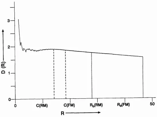
for the Full and Reduced Morphologies, the second and fourth data sets as presented in Figure 9.2(b) and (d). From equation (8.13), we have plotted the signatureD(R)against R and this is shown in Figure 9.4. This signature relates to the Full Morphology, but as the Reduced Morphology is a subset of this, the figure is relevant to both. The regional boundaries differ in that Rb

=

47.424 for the Full, Rb

=

28.071 for the Reduced, and these are also

indicated in Figure 9.4. At these values of R, the dimension for the Full system can be calculated as 1.756 in comparison with 1.704 for the Reduced. However, it is clear from Figure 9.4 that a better value of R to take would be the mean value C(Rb ), and these yield dimensions of D{C(Rb )} of 1.845

for C(18.590), the Full data set, in contrast to 1.856 for C(14.185) for the Reduced set. These estimates are close to and consistent with the regression estimates in Tables 9.2 to 9.5, and some exploration of the signature in Figure 9.4 reveals that in the region of the origin, the estimates of dimension are volatile, although by R=9, these estimates have settled to aroundD(9) = 1.85. Clearly the mean values of C(Rb ) are the most appropriate to use.

Together with the estimates of the simulations using the DLA and DBM methods in the two previous chapters, these signature functions have pro-ved to be the most robust methods of estimation.

The entropy estimation also produces well-fitting models with dimension values which accord to the results so far. These estimations involve solving equations (9.42) or (9.43) for the parameterT]by some non-linear

method-here we use the Newton-Raphson method - then using Table 9.1 to calcu-late the dimensions D (= 1+ T]). Two estimates are made for each of the

four data sets, these estimates being based on solving for the constraint in equation (9.42), then (9.43). All four data sets with their exclusions as given previously in Tables 9.2 to 9.5 are used in the estimation, thus giving 44 estimates of D in total. These results are shown in Table 9.6.In this table, under each dimension vallie, we first give the coefficient of determination

(100r2_{) for the predictions of the incremental population model which is}

3

g

°1

I

50

I

R~FM)

C(RM) o

O-+---r---l---~ I

C(FM)

R---.~

Table 9.6.

Entropy estimates of the dimension

Zonal system Full Morphology Zonal Morphology Reduced Morphology No. of Equations No. of Equations No. of Equations No. of Equations zones (9.42) (9.43) rings (9.42) (9.43) rings (9.42) (9.43) rings (9.42) (9.43) 80 1.132 1.703 25 0.898 0.621 25 1-.085 0.822 25 1.245 1.029

01.8 01.9 00.9 00.1 00.8 00.3 08.1 01.7

99.8 99.8 94.6 96.5 95.1 96.1 97.6 98.0

77 1.134 1.064 24 0.698 0.422 24 0.940 0.689 24 1.151 0.947

01.3 01.4 08.4 04.1 00.2 00." 02.7 04.8

99.8 99.8 95.9 97.1 95.6 96.4 97.7 98.1

71 1.188 1.134 15 1.405 1.252 13 1.942 1.973 18 1.640 1.544

03.5 03.6 39.4 44.2 94.3 94.4 66.5 68.2

99.8 99.8 98.7 99.1 99.9 99.9 99.3 99.4

68 1.199 1.130 14 1.283 1.157 12 1.972 1.990 17 1.614 1.152

02.8 02.9 21.7 24.5 93.1 93.1 59.2 60.8

99.8 99.8 98.9 99.2 99.9 99.9 99.3 99.4

9 1.870 1.829 10 1.882 1.912 14 1.881 1.870

93.3 93.6 94.3 94.4 90.6 90.6

99.8 99.8 99.9 99.9 99.8 99.8

8 1.838 1.803 9 1.910 1.931 13 1.903 1.890

90.3 90.5 92.6 93.0 88.4 88.4

99.8 99.8 99.9 99.9 99.8 99.8

Note:the first line of each cell is the fractal dimension, the second line is100r2_{for the increment of population, and the third line is}

100r2_{for the cumulative population.}

the form in which the model is specified in equation (9.41), and below this, we give the sam~coefficient for the population in cumulative form.

The results are similar to those in Tables 9.2 to 9.5 in that the Zonal System data performs least well. The Full, Zonal and Reduced Morphology data sets give parameter values and fits which are both good and similar to one another, and there is a consistent increase in the performance of all models as zones or rings are progressively excluded from the estimation. Of the 44 estimates, eight fall below D= 1 and none is greater than 2. As in previous estimates using regression, the best fits are those obtained when the most zones or rings are excluded. These results again strengthen our confidence in various hypotheses that suggest that cities never fill their two-dimensional space in which they grow, regardless of any vertical growth into the third dimension which has occurred within the last century, and that their fractional dimension lies between 1.5 and 1.8. Moreover, if the models and data sets to which they are applied are correctly specified, it is easy to give order of magnitude estimates for the density and dimension parameter values before the analysis begins.

9.9 Fractals and City Size

func-tional forms which have dominated social physics, the negative exponential which has become the conventional wisdom for representing density and interaction, and the inverse power which was associated with much early research. Notwithstanding our view that the inverse power function has less direct but important properties which have hitherto hardly been exploited or even recognized, the parameters of both functions reflect the properties of the space within which such functions are defined. However, it is clear that the parameters of the inverse power function are direct ures of the extent to which the phenomena whose density is being meas-ured, fills the space available, and using arguments from urban allometry, the link between such functions and fractal geometry can be made. Thus the function used determines the form of the system being modeled, and it is in this sense that we say 'form follows function'.

The empirical work in this chapter in which the inverse power function has been fitted to population density profiles in the city of Seoul has pro-duced quite startling results. Although all the theory we have developed in the last three chapters suggests that cities have a fractional dimension between 1 and 2, we did not expect our results to be quite so conclusive, over such a large range of scaling relations and estimation methods. Using the four data sets and variants of these based on excluding certain obser-vations, we have provided 136 estimates of the dimension D and density parameter <x. Of these, only 11 fall outside the postulated range 1

<

D

<

2, and these are all less than1.Ifwe look at the results based on excluding the most problematic observations, of the 24 values of the dimension pro-duced, 21 fall within the range 1.566 to 1.940, thus suggesting that the 'true' value of the dimension must be nearer 2 than 1.

However, perhaps the most important value of this analysis is not in demonstrating the consistency of results produced by both theoretical and empirical analysis, but in the need to be extremely careful in the way data are collected and density defined. Strictly, we need data bases in which every household and household size is recorded in terms of its location before we can develop any definitive analysis of density which exploits the fractal model most appropriately. This represents an immense task, but with better data and data systems becoming available, it is now within the bounds of feasibility. On both the theoretical and empirical sides of this argument, we also need to explore the link between entropy, information and dimension (Takayasu, 1989); for in doing so, we are likely to generate a clearer picture of the role of the conventional model of population density based on the negative exponential, as well as exploring further the proper-ties of the inverse power function. This will also enable us to link our approach to the mainstream where entropy and utility maximizing are widely used in the derivation and estimation of spatial economic, urban and transportation models.