APPLICATIONS OF STOCHASTIC MODELS IN ANALYSIS OF REAL DATA FOR FIRST BIRTH INTERVAL

(1)

-197-

Aryabhatta Journal of Mathematics & Informatics Vol. 6, No. 1, Jan-July, 2014 ISSN : 0975-7139 Journal Impact Factor (2013) : 0.489

APPLICATIONS OF STOCHASTIC MODELS IN ANALYSIS

OF REAL DATA FOR FIRST BIRTH INTERVAL

Shilpi Tanti

Assistant Professor, School of Business Sciences, University of Science and Technology, Meghalaya E-mail: shilpi.tanti@gmail.com.

ABSTRACT:

The levels and trends of human fertility can be obtained from the descriptive study of the real data. But some inherent characteristics of this phenomenon namely fecundability, sterility, etc. can be estimated only by applying appropriate models to the real data. Here, an attempt has been made to explore the uses and importance of the stochastic models relating to human fertility through real data. In this study, different probabilistic models have been considered to estimate the parameters by applying them to the data of the First Birth Interval in different major states of India obtained from National Family Health Survey - III.

Key Words: Stochastic process, Moment estimator, Truncated distributions etc.

1. INTRODUCTION:

A model is a mathematical abstract form of a real phenomenon, which includes the variables that may account for the explanation of the aspects taken into account. Modeling is one of the possible forms of scientific approach, often used in social sciences and particularly in demography to understand fertility, mortality, migration, nuptiality and other demographic measures. Broadly, a mathematical model is classified into two categories namely, Deterministic model and Stochastic model.

A model for a physical phenomenon is formulated keeping in mind that it embodies the essential features of the process. For this, a model builder generally makes certain assumptions about the process based on his/her experience and intuition and tries to describe the behavior of the process in terms of mathematical equations. The three important uses of the models are:

i) It can be used for prediction purposes. In fact, the phenomenon may have different components which may be inter-related and the model incorporates all these relationships in terms of a set of mathematical equations. Thus, a model provides a method for investigating the possible consequences in the process due to various alterations in the determinants of the process.

ii) It can be used for estimation of the parameters of the process by applying it to observed data relating to the process. These parameters will provide information about some unobserved characteristics of the process. iii) It can be used for explaining certain apparent inconsistencies in the observed data relating to the phenomenon

under consideration.

(2)

Shilpi Tanti

-198-

FBI has some unique features to investigate since usually females don’t like to use contraception to postpone the first birth and there is lower chance of recall lapse in reporting the time of first birth as it is the most important event in the life of the female. The nature of FBI is again somewhat different from other birth intervals as it is not influenced by the post-partum amenorrhea (PPA) period and thus it is generally studied separately from birth intervals of higher order.

The length of FBI depends on the conception rate or fecundability of the females. The terms fecundability and conception rate are dependent on time, whether it is taken as discrete or continuous. If unit of time is taken as one month then the conception rate may be interpreted as fecundability. If the unit of time is taken as one year then it is known as yearly conception rate. Conception rate is analogous to hazard rate used in life testing problem. Conception rate is the risk of conception in time (t, t +Δt) under the condition that conception has not occurred in time(0, t). The probability that an event will occur during a time interval is proportional to the length of that time interval.

Keeping the primacy of the models, the present paper focuses on the uses and importance as well as comparison of various stochastic models of first conceptive delay followed by the distribution of first birth interval (FBI), in particular, to the females of different ages at marriage of specific marital duration.

2. MODELS & THE ASSUMPTIONS:

Conception rate is estimated many times from the data ontime for first conception through the technique of probability modeling where the event of occurrence of conception is assumed as random. Generally, data on first conception time are not available and these are obtained from the data on FBI on the assumption that there is one to one correspondence between conception and live birth. Hence, subtracting gestation period (9 months or 0.75

years) from the duration of FBI, one may have data of first conception. In literature, there are many crucial assumptions for the indirect estimation of conception rate. These assumptions are broadly classified into three categories: (Pratap, 2011)

I. Conception rate of each female is constant till the time of first conception and population is homogeneous with respect to conception rate.

II. Conception rate of each female is constant till the time of first conception but population is heterogeneous with respect to conception rate.

III. Conception rate is time dependent (time being measured from the time of marriage).

It is expected that assumptions (I) and (II) may be more appropriate for females of higher ages at marriage depending on homogeneity and heterogeneity in the population while the assumption (III) may be more appropriate for females of lower ages at marriage, say less than 15-16 years, as it indirectly incorporates the adolescent sterility and other social norms and taboos associated with it (Pathak, 1978; Pathak, 1981; Nair, 1983; Nair, 1983a; Bhattacharya, 1988). The fertility behavior of a female who married in her adolescent ages becomes quite different than that of a female who married at later ages on account of biological phenomena. Under this situation, conception rate may be assumed to have an increasing trend over time or increasing up to some level and then remaining constant.

(3)

Applications of Stochastic models inanalysis of real data for first birth interval

Model I:

Model I is derived on the assumption that conception rate is constant for each female from marriage to first conception. Let 𝑋 denote the time between marriage and the first conception. If the time is treated as continuous then the assumption (𝐼) implies that the chance of conception between time 𝑡 and (𝑡 + 𝛥𝑡) is 𝜆. 𝛥𝑡 + 𝑂(𝛥𝑡) with p.d.f of 𝑋 as

𝑓1 𝑥 = 𝜆𝑒

−𝜆𝑥

0 ; 𝑜𝑡𝑕𝑒𝑟𝑤𝑖𝑠𝑒 ; 𝑥 > 0, 𝜆 > 0, …. (2.1)

Here λ represents the conception rate per unit of time.

Model II:

The females under study are usually coming from various socio-economic, demographic and biological backgrounds. Hence, the assumption of constant conception rate may not be reasonable. In a study, the conception rate showed a declining trend with increasing time for females of higher ages at marriage (Pratap, 2011). This feature cannot be completely removed by disaggregation and is usually viewed as a selection effect in which the more fecund females tend to conceive first. To capture this selection effect, it may be assumed that for a female 𝑋

(duration from marriage to first conception) follows the density given in Equation (2.1), where λ varies in the population from female to female and 𝜆 follows a probability distribution with p.d.f. 𝑓(𝜆). Hence, if a female under study is randomly selected from the population, then the unconditional distribution of 𝑋 is given as

𝑓2 𝑥 = 𝜆𝑒−𝜆𝑥𝑓 𝜆 𝑑𝜆 ;

∞

0 …. (2.2)

This mixture can take a parametric form or be left arbitrary. The most widely published model for incorporating heterogeneity in conception rateis Pearson type III distribution. The choice of this distribution is due to its flexibility, mathematical applicability and interpretation.

𝑓 𝜆 = 𝛽𝛼

𝛤 𝛼 𝜆

𝛼−1 _𝑒−𝜆𝛽_{; 𝛼 > 0, 𝛽 > 0} _{…. (2.3)}

where𝛼 and 𝛽 are positive constants and 𝛤 (. ) is the gamma function. Under this situation,𝑓2 𝑥 becomes

𝑓2 𝑥 =

𝛼 𝛽𝛼

(𝛽 +𝑥 )(𝛼 +1) ; 𝛼 > 0, 𝛽 > 0, 𝑥 > 0 …. (2.4)

It should be noted that 𝜆 differs from female to female and it is constant over time for a fixed female.

Model III:

Model III is derived on the basis of the assumption that conception rate is𝜆 𝑡 , which is a function of time t. Under this situation;

𝑓3 𝑥 = 𝜆(𝑡)𝑒

− 𝜆) 𝑡 𝑑𝑡₀𝑥

0 ; 𝑜𝑡𝑕𝑒𝑟𝑤𝑖𝑠𝑒 ; 𝑥 > 0 …. (2.5)

If 𝜆 𝑡 is assumed as a linear function of time, i.e., 𝜆 𝑡 = 𝑎 + 𝑏𝑡, then the probability density function of Xis given by

𝑓3 𝑥 = (𝑎 + 𝑏𝑥)𝑒

−(𝑎𝑥 +𝑏𝑥2

2)

0 ; 𝑜𝑡𝑕𝑒𝑟𝑤𝑖𝑠𝑒 ; 𝑥 > 0

…. (2.6)

Model IV:

(4)

Shilpi Tanti

-200-

i) The cohort of females is a mixture of two groups - (a) the adolescent sterile group (those who are not biologically mature at the time of marriage but are exposed to the risk of Ovulation) and (b) the ovulation group (those who are biologically mature at the time of marriage and are exposed to the risk of conception). Let 𝜃 and 1 − 𝜃 be the proportions of two types of females respectively.

ii) For group (a) females, the interval between marriage and the time of ovulatory menstruation follows a negative exponential distribution with parameter µand the duration of waiting time to conception from ovulatory menstruating state, follows a negative exponential distribution with parameter 𝜆.

iii) Group (b) female moves to the state of conception according to a negative exponential distribution with parameter 𝜆.

The probability density function of 𝑋 is given by;

𝑓4 𝑥 = 𝜃𝑓 𝑥1+ 𝑥2 + 1 − 𝜃 𝑓 𝑥2 ; 0 ≤ 𝜃 ≤ 1 …. (2.7)

where𝑋1 is the waiting time required for a female to move to the state of ovulation from the adolescent sterile state

and 𝑋2 is the waiting time for a female to move to the state of first conception from the start of ovulation state. By

solving the above equation, we get;

𝑓4 𝑥 = 𝜃𝜇𝜆 𝜆 −µ 𝑒

−𝜇𝑥 _{− 𝑒}−𝜆𝑥_{+ 1 − 𝜃 𝜆𝑒}−𝜆𝑥_{; 0 ≤ 𝜃 ≤ 1,} _{𝜇 > 0,} _{𝜆 > 0}

= 𝛼𝜇𝑒−𝜇𝑥 + 𝛽𝜆𝑒−𝜆𝑥 …. (2.8) Where 𝛼 = 𝜃𝜆

𝜆−𝜇 and 𝛽 = 1 − 𝛼.

The procedures of the estimation of the parameters involved in all the four models are briefly described in the following section.

3. ESTIMATION OF THE PARAMETERS OF THE MODELS:

In Model I, the maximum likelihood estimator as well as moment estimator of λ is 1

𝑋 , where 𝑋 is sample mean. In

this paper, the method of maximum likelihood (M.L.) is being proposed for estimation of parameters involved in Models II, III and IV. The moment estimators of the parameters involved in Model II have disadvantage as the moment estimator does not exist for 𝛼 ≤ 2. Hence, maximum likelihood(M.L.) estimator for the parameters of this continuous time model for first conception is preferable. It may be noted that Nath etal. (1995) proposed the method of moments to estimate the parameters of the model but here the method of M. L. is being proposed. The procedure can be briefly described as below:

Let 𝑥1 , 𝑥2, … , 𝑥𝑛 be a random sample of size 𝑛 from the population with density function𝑓𝑖 𝑥 ; 𝑖 = 2, 3, 4. The

logarithm of the likelihood functions for Model II, III and IV are given in Expressions 3.1-3.3.

log2𝐿 = 𝑛𝑙𝑜𝑔𝛼 + 𝑛𝛼𝑙𝑜𝑔𝛽 − 𝛼 + 1 𝑙𝑜𝑔(𝑥𝑖 + 𝛽) 𝑛

𝑖=1

, ⋯ (3.1)

𝑙𝑜𝑔3𝐿 = log⁡(𝑎 + 𝑏𝑥𝑖 𝑛

𝑖=1

) − 𝑎 𝑥𝑖 𝑛

𝑖=1

− 𝑏 𝑥𝑖 2

2 𝑛

𝑖=1

, … (3.2)

𝑙𝑜𝑔4𝐿 = log 𝛼𝜇𝑒−𝜇 𝑥𝑖+ 𝛽𝜆𝑒−𝜆𝑥𝑖 , … (3.3) 2

(5)

The above likelihoods are used to estimate the parameters of the models when marital duration is infinite. But in this study specific finite marital duration say, T, is considered, hence the M.L. estimates of the parameters are obtained by fitting the truncated form of the distributions and the form of the truncated distributions are as follows:

𝑓2∗ 𝑥 = 𝑓2(𝑥) 𝐹2(𝑇)

; 0 ≤ 𝑥 ≤ 𝑇, … (3.4)

𝑓3∗ 𝑥 = 𝑓3(𝑥) 𝐹3(𝑇)

; 0 ≤ 𝑥 ≤ 𝑇, … (3.5)

𝑓₄∗ 𝑥 =𝑓4(𝑥) 𝐹4(𝑇)

; 0 ≤ 𝑥 ≤ 𝑇, … (3.6)

Now, the log likelihood functions of the truncated distributions having respective densities 𝑓_𝑖∗ 𝑥 ; 𝑖 = 2, 3, 4 are as follows:

𝑙𝑜𝑔2∗𝐿 = 𝑛𝑙𝑜𝑔𝛼 + 𝑛𝛼𝑙𝑜𝑔𝛽 − 𝛼 + 1 log⁡(𝑥𝑖 + 𝛽) − 𝑛𝑙𝑜𝑔(1 − 𝛽𝛼 (𝑇 + 𝛽)𝛼) 𝑛

𝑖=1

, ⋯ (3.7)

𝑙𝑜𝑔3∗𝐿 = log⁡(𝑎 + 𝑏𝑥𝑖 𝑛 𝑖=1 ) − 𝑎 𝑥𝑖 𝑛 𝑖=1 − 𝑏 𝑥𝑖 2 2 𝑛 𝑖=1

− 𝑛𝑙𝑜𝑔(1 − 𝑒− 𝑎𝑇 +𝑏

𝑇2

2 _{) , … (3.8)}

𝑙𝑜𝑔4∗𝐿 = log 𝛼𝜇𝑒−𝜇 𝑥𝑖+ 𝛽𝜆𝑒−𝜆𝑥𝑖 − 𝑛𝑙𝑜𝑔(1 − 𝛼𝑒−𝜇𝑇 − 𝛽𝑒−𝜆𝑇) , … (3.9) 𝑛

𝑖=1

The M. L. estimates of the parameters𝛼 and 𝛽 involved in Model II are obtained from the Equations 3.10-3.11 given below

𝑆21 = 𝜕𝑙𝑜𝑔𝐿

𝜕𝛼 = 0 ; ⋯ (3.10) 𝑆22 =

𝜕𝑙𝑜𝑔𝐿

𝜕𝛽 = 0 ; ⋯ (3.11)

Solving the above equations, we obtain

𝑛

𝛼+ 𝑛𝑙𝑜𝑔𝛽 − log⁡(𝑥𝑖 𝑛

𝑖=1

+ 𝛽) = 𝑛 𝜕

𝜕𝛼𝑙𝑜𝑔 1 − 𝛽𝛼

𝑇 + 𝛽 𝛼 ; ⋯ (3.12)

𝑛𝛼

𝛽 − 𝛼 + 1 1 𝑥𝑖+ 𝛽 𝑛

𝑖=1

= 𝑛 𝜕

𝜕𝛼𝑙𝑜𝑔 1 − 𝛽𝛼

𝑇 + 𝛽 𝛼 ; ⋯ (3.13)

The M. L. estimates of the parameters 𝑎 and 𝑏of Model III are obtained from the following equations:

𝜕𝑎 = 0 , … (3.14) 𝑆32 =

𝜕𝑙𝑜𝑔𝐿

𝜕𝑏 = 0 , … (3.15)

i.e.; 1 (𝑎 + 𝑏𝑥𝑖) 𝑛 𝑖=1 = 𝑥𝑖 𝑛 𝑖=1 + 𝑛𝑇𝑒 −𝑎𝑇

1 − 𝑒− 𝑎𝑇 +𝑏

𝑇2

2

; … (3.16)

𝑥𝑖 (𝑎 + 𝑏𝑥𝑖) 𝑛 𝑖=1 = 𝑥𝑖 2 2 𝑛 𝑖=1 + 𝑛𝑇

2_𝑒−𝑏𝑇₂2

2(1 − 𝑒− 𝑎𝑇 +𝑏

𝑇2

2 ₎

; … (3.17)

Again, the estimates of the parameters 𝜃, µ and 𝜆 involved in Model IV are obtained by solving the following equations:

(6)

Shilpi Tanti

-202-

𝜕µ = 0 , … (3.19)

𝜕𝜆 = 0 , … (3.20)

i.e.;

𝜇𝑒

−𝜇 𝑥𝑖_{− 𝜆𝑒}−𝜆𝑥𝑖

𝛼𝜇𝑒−𝜇 𝑥𝑖+ 𝛽𝜆𝑒−𝜆𝑥𝑖

𝑛

𝑖=1

= 𝑛(𝑒

−𝜆𝑇 _{− 𝑒}−µ𝑇₎

1 − 𝛼𝑒−𝜇𝑇 _{− 𝛽𝑒}−𝜆𝑇; … (3.21)

𝜃𝜆 𝜇 − 𝜆 𝑥𝑖𝑒

−𝜇 𝑥𝑖

𝛼𝜇𝑒−𝜇 𝑥𝑖 + 𝛽𝜆𝑒−𝜆𝑥𝑖

𝑛

𝑖=1

=𝑛{ 𝜆 −µ 𝜃𝜆𝑇𝑒

−µ𝑇_{+ 𝜃𝜆 𝑒}−𝜆𝑇_{− 𝑒}−µ𝑇_}

1 − 𝛼𝑒−𝜇𝑇 _{− 𝛽𝑒}−𝜆𝑇 ; … (3.22)

𝜇

2_{− 𝜃𝜆}2_{− 2𝜆}_µ_{+ 2𝜃𝜆}_µ_{− 𝜆}3_{1 − 𝜃 + 𝜇}2_{𝜆 + 𝜃}_µ_𝜆2_𝑥

𝑖 𝑒−𝜆𝑥𝑖 − 𝜃𝜇2𝑒−𝜇 𝑥𝑖

𝛼𝜇𝑒−𝜇 𝑥𝑖+ 𝛽𝜆𝑒−𝜆𝑥𝑖

𝑛

𝑖=1

=𝑛{ 𝜆 −µ− 𝜃𝜆 𝑇(𝜆 −µ)𝑒

−𝜆𝑇 _{+ 𝜃}_µ_𝑒−µ𝑇_{− 𝑒}−𝜆𝑇_}

1 − 𝛼𝑒−𝜇𝑇 _{− 𝛽𝑒}−𝜆𝑇 ; … (3.23)

These sets of expressions (Expressions 3.12-3.13, 3.16-3.17 and 3.21-3.23) are quite complicated and no explicit solution exists. However, M.L. estimates of the parameters are computed by Newton Raphson method taking certain guess values of the parameters through the expression of log likelihood function using R-software.

4. APPLICATION:

The data utilized for the present study have been taken from National Family Health Survey III (NFHS-III). NFHS provides the data on marriage to FBI (in months), age at marriage (in years), date of marriage (in CMC) and date of the survey (in CMC), etc. The data on waiting time to first conception are obtained by subtracting nine months from the interval from marriage to first birth assuming one to one correspondence between conception and live birth. Here, only those females are considered whose marriage took place at least seven years prior to the reference date of the survey. This is done to take account the truncation effect, as discussed in Shepset. al (1970). It is well known that conception outside wedlock is generally not accepted in Indian society; hence the negative FBI durations are excluded from the study. Again, the FBI durations of less than nine months are also excluded from the study since in this study the gestation period is taken as nine months. Females are divided into two groups according to their age at marriage (lower ages at marriage (<16 years) & higher ages at marriage (>=16 years)). Models are then applied to the data of first conception for different major states viz., Bihar, Uttar Pradesh, Madhya Pradesh, Rajasthan, Assam, Orissa, Maharashtra, West Bengal, Andhra Pradesh, Karnataka, Kerala and Tamil Nadu situated in different regions of the country. Models I and II are applied to the data of first conception for the females whose age at marriage >=16 years, whereas, Model III and IV are applied to the data of first conception for the females whose age at marriage is <16 years.

5. DISCUSSION & CONCLUSIONS:

(7)

themselves. Thus, the assumption of heterogeneity with respect to conception rate seems to be more appropriate for describing the phenomenon of time of first conception for females of higher ages at marriage.

However, one natural question arises;“Why is Model I fitting well to some of the states?”The answer of this question may be thatfemales of those states may have same social status and each of them may have gone through the similar socio-cultural norms and taboos after marriage i.e., population is more or less homogeneous.

Model II explains the variation in conception rate among the females in different states of the country. It has been observed that females of the states viz., Assam, Maharashtra, Andhra Pradesh, Karnataka, Kerala, and Tamil Nadu are more heterogeneous than the rest considered parts (see Fig 1). It may be due to the socio-cultural variations between the states. Thus, with the help of Model II, it has become possible to observe the heterogeneity in the population.

Tables 7-11 present the observed and expected frequencies of waiting time to first conception, the estimated parameters and the respective value of chi-square as well as Akaike Information Criterion (AIC and AIC corrected) values under Model III and Model IV for females of lower ages at marriage. These tables show that there is no significant difference between the chi-square values of Model III and Model IV, both are fitting quite well.Model III is derived on the assumption that conception rate is a linear function of time𝑡. As it is mentioned earlier that FBI signifies couple's fertility at early stages of married life and in traditional society like India, the early part of married life is governed by large number of socio-cultural norms and taboos. These social norms and taboos decrease with the passage of time of marriage. Along with these social norms and taboos, when the age at marriage is low, there is one most important biological factor that influences this duration variable, is referred to as adolescent sterility. Model III indirectly incorporates all these factors together by considering conception rate as time dependent.

Model IV is based on the assumption that the females of lower ages at marriage are a mixture of two groups: the adolescent sterile group and the ovulation group. In case of lower ages at marriage, the most important chance mechanism which influences the fertility behavior of female is adolescent sterility. It is worthwhile to mention that the extent of all social norms and taboos can be reduced by one's effort but the extent of adolescent sterility cannot be reduced by one’s effort. Model IV ascertains the extent of adolescent sterility. May be due to this possible reason, Model IV performs well than Model III when both of them are applied to the real data. But the beauty of Model III is that in addition to its mathematical simplicity; it explains the phenomena very well.

(8)

Shilpi Tanti

-204-

Here, all the four models have been applied on various data sets of waiting time to first conception and on the basis of the values of chi-square, it can be concluded that whether a model is appropriate or not. Appropriateness of a model depends upon the assumptions under consideration. If a model is appropriate for a process, then on an average it will fit the data of that process. Sometimes, there may be many models for the same phenomenon and they fit the data well. But, it does not mean that all the models are correct. Therefore, one must have logical interpretation of the parameters involved in the probability models. Consequently these parameters are used as alternative measures of various aspects of the process under consideration. These estimates can be easily compared so that valid and informative conclusions can be drawn.

Thus, it may be said that probability models are very useful and play an important role for explaining the real phenomenon. The variability, uncertainty and complexity of the phenomenon under study can be deeply understood with the help of the models and on the basis of these probability models, decision makings are validated. Some unobserved characteristics can be estimated with the applications of the models to the real data. For example; the extent of heterogeneity as well as homogeneity in the population, how conception rate varies over time and the proportion of adolescent sterility can be estimated. These findings may be helpful for policy makers to frame appropriate policies and their implementation.

6. TABLES & FIGURE:

Table 1: Observed and expected frequencies of waiting time to conception for Bihar and Uttar Pradesh under Model I and Model II for females of higher ages at marriage (>=16 years)

C. I.* (in years)

States

Bihar Uttar Pradesh

Observed Model I Model II Observed Model I Model II

0-1 334 332.9 335.7 1446 1426.5 1436.3

1-2 207 195.5 193.7 824 801.7 795.1

2-3 106 114.8 113.0 399 450.6 444.5

3-4 70 67.4 66.6 271 253.2 250.8

4-5 32 39.6 39.7 147 142.3 142.8

5-6 25 23.2 23.8 73 89.9 82.1

6-7 13 13.6 14.5 39 44.9 47.5

Total 787 787.0 787.0 3199 3199.0 3199.0

𝜒_{(𝑐𝑎𝑙 )}2 _χ

5

2_{= 3.068} _χ

4

2_{= 3.210} _χ

5

2_{= 9.583} _χ

4

2_{= 10.049}

Estimated parameters

𝜆 = 0.532 𝛼 = 26.182

𝛽 = 48.472 𝐸 𝜆 = 0.540

𝑉 𝜆 = 0.011

𝜆 = 0.576 𝛼 = 34.363

𝛽 = 58.854 𝐸 𝜆 = 0.584

𝑉 𝜆 = 0.010

AIC 2385.066 2386.900 9346.945 9348.513

AICc 2385.063 2386.884 9346.940 9348.509

(9)

Table 2: Observed and expected frequencies of waiting time toconception for Madhya Pradesh and Rajasthan under Model I and Model II for females of higher ages at marriage (>=16 years)

C. I. (in years)

States

Madhya Pradesh Rajasthan

0-1 864 908.2 918.5 386 426.0 430.9

1-2 591 509.2 508.6 312 264.0 264.3

2-3 284 285.4 282.4 191 163.6 162.4

3-4 148 160.0 157.2 87 101.4 100.0

4-5 89 89.7 87.7 51 62.9 61.7

5-6 33 50.3 49.1 28 39.0 38.1

6-7 22 28.2 27.5 26 24.1 23.6

Total 2031 2031.0 2031.0 1081 1081.0 1081.0

𝜒_{(𝑐𝑎𝑙 )}2 _χ

5

2_{= 23.529} _χ

4

2_{= 23.530} _χ

5

2_{= 24.559} _χ

4

2_{= 24.779}

𝜆 = 0.579 𝛼 = 130.649

𝛽 = 221.773 𝐸 𝜆 = 0.589 𝑉 𝜆 = 0.003

𝜆 = 0.478 𝛼 = 126.965

𝛽 = 260.841 𝐸 𝜆 = 0.487 𝑉 𝜆 = 0.002

AIC 5922.795 5926.361 3417.122 3419.769

AICc 5922.794 5926.355 3417.120 3419.758

Table 3 Observed and expected frequencies of waiting time to conception for Assam and Orissa under Model I and Model II for females of higher ages at marriage (>=16 years)

C. I. (in years)

States

Assam Orissa

0-1 569 562.3 335.7 672 648.9 665.1

1-2 246 243.9 193.7 328 329.8 316.9

2-3 98 105.8 113.0 149 167.6 158.5

3-4 34 45.9 66.6 75 85.2 82.8

4-5 21 19.9 39.7 49 43.3 44.9

5-6 16 8.6 23.8 19 22.0 25.2

6-7 6 3.7 14.5 16 11.2 14.6

Total 990 990.0 787.0 1308 1308.0 1308.0

𝜒_{(𝑐𝑎𝑙 )}2 _χ

5

2_{= 11.464} _χ

4

2_{= 7.526} _χ

5

2_{= 7.353} _χ

4

2_{= 3.810}

𝜆 = 0.835 𝛼 = 5.300

𝛽 = 5.562

𝐸 𝜆 = 0.877

𝑉 𝜆 = 0.985

𝜆 = 0.677 𝛼 = 9.532

𝛽 = 13.278

𝐸 𝜆 = 0.718

𝑉 𝜆 = 0.054

(10)

Shilpi Tanti

-206-

AICc 2298.849 2289.495 3506.631 3505.102

Table 4: Observed and expected frequencies of waiting time to conception for Maharashtra and West Bengal under Model I and Model II for females of higher ages at marriage (>=16 years)

C. I. (in years)

States

Maharashtra West Bengal

0-1 1751 1617.0 1732.5 976 955.0 978.4

1-2 606 713.0 595.5 455 453.0 432.6

2-3 230 314.4 263.0 205 214.9 202.6

3-4 152 138.6 135.5 84 101.9 99.7

4-5 84 61.1 77.5 43 48.4 51.2

5-6 33 27.0 47.8 26 22.9 27.4

6-7 27 11.9 31.3 18 10.9 15.1

Total 2883 2883.0 2883.0 1807 1807.0 1807.0

𝜒_{(𝑐𝑎𝑙 )}2 _χ

5

2_{= 80.240} _χ

4

2_{= 12.260} _χ

5

2_{= 9.744} _χ

4

2_{= 5.595}

𝜆 = 0.835 𝛼 = 2.587

𝛽 = 2.494

𝐸 𝜆 = 1.037

𝑉 𝜆 = 0.416

𝜆 = 0.746 𝛼 = 9.884

𝛽 = 12.418

𝐸 𝜆 = 0.796

𝑉 𝜆 = 0.064

AIC 6794.443 6704.183 4554.119 4550.142

AICc 6794.442 6704.179 4554.117 4550.135

Table 5: Observed and expected frequencies of waiting time to conception for Andhra Pradesh and Tamil Nadu under Model I and Model II for females of higher ages at marriage (>=16 years)

C. I. (in years)

States

Andhra Pradesh Tamil Nadu

0-1 964 926.7 974.1 1547 1406.4 1529.1

1-2 449 454.7 413.2 364 525.1 377.1

2-3 167 223.1 198.4 159 196.0 155.2

3-4 111 109.5 104.5 77 73.2 80.5

4-5 71 53.7 59.1 47 27.3 47.8

5-6 22 26.4 35.4 26 10.2 30.9

6-7 23 12.9 22.2 22 3.8 21.4

Total 1807 1807.0 1807.0 2242 2242.0 2242.0

𝜒_{(𝑐𝑎𝑙 )}2 _χ

5

2_{= 29.822} _χ

4

2_{= 16.078} _χ

5

2_{= 196.189} _χ

4

2_{= 1.740}

(11)

parameters _{𝛽 = 5.096}

𝐸 𝜆 = 0.904 𝑉 𝜆 = 1.208

𝛽 = 1.054

𝐸 𝜆 = 1.515 𝑉 𝜆 = 1.437

AIC 4694.871 4675.915 4516.769 4296.179

AICc 4694.869 4675.908 4516.768 4296.174

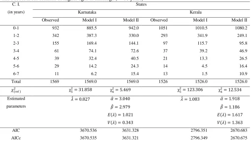
Table 6: Observed and expected frequencies of waiting time to conception for Karnataka and Kerala under Model I and Model II for females of higher ages at marriage (>=16 years)

C. I. (in years)

States

Karnataka Kerala

0-1 932 885.5 942.0 1051 1010.5 1080.2

1-2 342 387.3 330.0 293 341.9 249.1

2-3 155 169.4 144.1 97 115.7 95.8

3-4 61 74.1 72.6 37 39.2 46.9

4-5 39 32.4 40.5 21 13.3 26.5

5-6 29 14.2 24.3 14 4.5 16.4

6-7 11 6.2 15.4 13 1.5 10.9

Total 1569 1569.0 1569.0 1526 1526.0 1526.0

𝜒_{(𝑐𝑎𝑙 )}2 _χ

5

2_{= 31.858} _χ

4

2_{= 5.469} _χ

5

2_{= 123.306} _χ

4

2_{= 12.534}

𝜆 = 0.827 𝛼 = 3.040

𝛽 = 2.979 𝐸 𝜆 = 1.021

𝑉 𝜆 = 0.343

𝜆 = 1.083 𝛼 = 1.918

𝛽 = 1.186 𝐸 𝜆 = 1.617

𝑉 𝜆 = 1.363

AIC 3670.536 3631.328 2796.351 2670.683

AICc 3670.535 3631.321 2796.349 2670.675

Table 7: Observed and expected frequencies of waiting time to conception for Bihar and Uttar Pradesh under Model III and Model IV for females of lower ages at marriage (<16 years)

C. I. (in years)

States

Bihar Uttar Pradesh

Observed Model III Model IV Observed Model III Model IV

0-1 199 206.0 213.5 474 492.2 504.3

1-2 196 195.1 188.1 432 424.1 407.5

2-3 133 154.3 140.7 308 316.3 291.9

3-4 101 104.8 97.1 184 207.5 195.9

4-5 85 61.9 63.8 127 120.8 126.1

5-6 35 32.1 40.6 82 62.8 78.9

6-7 20 14.7 25.2 46 29.3 48.4

Total 769 769.0 769.0 1653 1653.0 1653.0

𝜒(𝑐𝑎𝑙 )2 χ42= 14.071 χ23= 10.783 χ42= 19.402 χ32= 5.151

(12)

Shilpi Tanti

-208- parameters _{𝑏 = 0.109} _{𝜆 = 0.617}

𝜃 = 0.589

𝑏 = 0.097 𝜆 = 0.624

𝜃 = 0.513

AIC 2703.188 2683.777 5698.941 5647.489

AICc 2703.172 2683.745 5698.948 5647.504

Table 8: Observed and expected frequencies of waiting time to conception for Madhya Pradesh and Rajasthan under Model III and Model IV for females of lower ages at marriage (<16 years)

C. I. (in years)

States

Madhya Pradesh Rajasthan

0-1 357 394.3 396.6 207 222.0 226.7

1-2 388 353.7 358.7 238 226.1 223.8

2-3 273 263.0 248.3 176 186.5 172.5

3-4 141 166.4 154.4 119 129.5 119.5

4-5 80 90.8 90.7 84 77.2 77.9

5-6 58 43.0 51.6 39 39.8 48.8

6-7 32 17.8 28.7 36 17.9 29.8

Total 1329 1329.0 787.0 899 899.0 899.0

𝜒_{(𝑐𝑎𝑙 )}2 _χ

4

2_{= 28.942} _χ

3

2_{= 12.415} _χ

4

2_{= 21.862} _χ

3

2_{= 6.423}

𝑎 = 0.289

𝑏 = 0.120

µ

= 0.635

𝜆 = 0.938

𝜃 = 0.617

𝑎 = 0.220

𝑏 = 0.119

µ

= 0.644

𝜆 = 0.645

𝜃 = 0.693

AIC 4457.000 4426.812 3191.852 3163.038

AICc 4457.009 4426.830 3191.838 3163.012

Table 9: Observed and expected frequencies of waiting time to conception for Maharashtra and West Bengal under Model III and Model IV for females of lower ages at marriage (<16 years)

C. I. (in years)

States

Maharashtra West Bengal

0-1 418 430.1 435.7 379 381.5 389.7

1-2 295 283.7 273.6 236 249.8 236.4

2-3 138 171.9 163.2 141 152.0 141.8

3-4 118 95.9 94.2 91 86.1 84.3

4-5 57 49.4 53.0 60 45.6 49.7

5-6 23 23.6 29.3 22 22.5 29.1

6-7 16 10.4 16.0 19 10.4 17.0

Total 1065 1065.0 1065.0 948 948.0 948.0

𝜒_{(𝑐𝑎𝑙 )}2 _χ

4

2_{= 16.745} _χ

3

2_{= 14.003} _χ

4

2_{= 13.507} _χ

3

(13)

Applications of Stochastic models inanalysis of real data for first birth interval Estimated

parameters

𝑎 = 0.502

𝑏 = 0.031

µ

= 0.717

𝜆 = 0.718

𝜃 = 0.314

𝑎 = 0.479

𝑏 = 0.062

µ

= 0.612

𝜆 = 0.612

𝜃 = 0.170

AIC 3255.406 3238.886 3053.203 2914.378

AICc 3255.394 3238.863 3053.191 2914.352

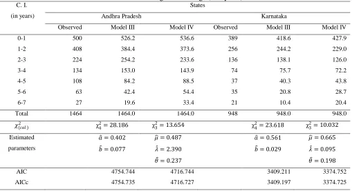
Table 10: Observed and expected frequencies of waiting time to conception for Andhra Pradesh and Karnataka under Model III and Model IV for females of lower ages at marriage (<16 years)

C. I. (in years)

States

Andhra Pradesh Karnataka

0-1 500 526.2 536.6 389 418.6 427.9

1-2 408 384.4 373.6 256 244.2 229.0

2-3 224 254.2 233.6 136 138.1 126.0

3-4 134 153.0 143.9 74 75.7 72.2

4-5 108 84.2 88.5 37 40.3 43.8

5-6 63 42.4 54.4 35 20.8 28.7

6-7 27 19.6 33.4 21 10.4 20.4

Total 1464 1464.0 1464.0 948 948.0 948.0

𝜒(𝑐𝑎𝑙 )2 χ42= 28.186 χ23= 13.654 χ42= 23.618 χ32= 10.032

𝑎 = 0.402

𝑏 = 0.077

µ

= 0.487

𝜆 = 2.390

𝜃 = 0.237

𝑎 = 0.561

𝑏 = 0.029

µ

= 0.665

𝜆 = 0.095

𝜃 = 0.198

AIC 4754.744 4716.744 3409.211 3374.752

AICc 4754.735 4716.727 3409.197 3374.725

Table 11: Observed and expected frequencies of waiting time to conception for Kerala and Tamil Nadu under Model III and Model IV for females of lower ages at marriage (<16 years)

C. I. (in years)

States

Kerala Tamil Nadu

0-1 82 90.4 92.8 350 357.1 365.0

1-2 60 52.5 48.6 151 149.4 137.8

2-3 28 29.6 26.7 60 64.8 57.6

3-4 15 16.2 15.6 25 29.2 28.1

4-5

19

15.3 20.3 15 13.6 16.4

5-6 15 6.6 11.0

6-7 8 3.3 8.1

Total 204 787.0 204.0 624 624.0 624.0

𝜒(𝑐𝑎𝑙 )2 χ2

2_{= 2.906} _χ

3

2_{= 4.062} _χ

4

2_{= 18.798} _χ

3

2_{= 3.902}

(14)

Shilpi Tanti

-210- parameters _{𝑏 = 0.027} _{𝜆 = 0.259}

𝜃 = 0.221

𝑏 = −0.039 𝜆 = 0.225

𝜃 = 0.175

AIC 615.401 610.186 1513.673 1497.314

AICc 615.341 610.066 1513.654 1497.276

𝝌_𝒕𝒂𝒃𝟐 = 𝟑. 𝟖𝟒𝟏 𝟏 𝒅. 𝒇. , 𝟓. 𝟗𝟗𝟏 𝟐 𝒅. 𝒇. , 𝟕. 𝟖𝟏𝟓 𝟑 𝒅. 𝒇. , 𝟗. 𝟒𝟖𝟖 𝟒 𝒅. 𝒇. , 𝟏𝟏. 𝟎𝟕𝟎 (𝟓 𝒅. 𝒇. )

Figure 1:Graph showing the heterogeneity in conception rate of female in some states of India:

ACKNOLWEDGMENT: The author would like to acknowledge Prof. R.C. Yadav & Prof. K.K. Singh for their valuable comments and also pay thank to DST centre for Inter-disciplinary Mathematical Sciences for financial assistance to carry out the research work.

REFERENCES:

[1] Gini, C.; Premieres recherchessur la fecondabilite de la femme.Proceedings ofthe International Mathematics

Congress,Toronto (1924).

[2] Henry, L.;Fondementstheoretiques des measures da la feconditenaturelle.Perue de 1 InstutInternational de

Statistique, 21: 135 (1953).

[3] Sheps, M.C., Menken, J.A., Ridley, J.C., Lingler, J.W.; Truncation effectin closed and open birth interval data.Journal of the American Statistical Association, 65(330), 678-693 (1970)

[4] Pathak, K.B.; An extension of the waiting time distribution of first conception. Journal of Biosciences, 10, 231{234 (1978)

[5] Pathak, K.B., Pandey, A.; Analytical model of human fertility with provision for adolescent sterility. Health

and Population-Perspectives and Issues, 7, 171{180 (1981)

[6] Gondotra, M.M., Das, N.; Age at menarche in an Indian population. Health and Population-Perspectives and

Issues, 5(3), 168-181 (1982)

[7] Nair, N.U.;On a distribution of first conception delays in the presence of adolescent sterility. Demography

India, 12, 209 (1983)

(15)

[9] Bhattacharya, B.N., Pandey, C.M., Singh, K.K.; Model for first birth interval and some social factors.Journal

of Mathematical Biosciences, 92,17-28 (1988)

[10] Nath, D.C., Land, K.C., Singh, K.K.; A waiting time distribution for the first conception and its application to a non-contracepting traditional society. Genus 51(1/2), 95{103 (1995)