Dyonic and magnetic black holes with rational nonlinear electrodynamics
S. I. Kruglov 1
Department of Physics, University of Toronto, 60 St. Georges St., Toronto, ON M5S 1A7, Canada
Department of Chemical and Physical Sciences, University of Toronto, 3359 Mississauga Road North, Mississauga, ON L5L 1C6, Canada
Abstract
The principles of causality and unitarity are studied within rational nonlinear electrodynamics proposed earlier. We investigate dyonic and magnetized black holes and show that in the self-dual case, when the electric charge equals the magnetic charge, corrections to Coulomb’s law and Reissner−Nordstr¨om solutions are absent. In the case of the magnetic black hole, the Hawking temperature, the heat capacity and the Helmholtz free energy are calculated. It is shown that there are second-order phase transitions and it was demonstrated that at some range of parameters the black holes are stable.
1
Introduction
The black holes (BHs) are real objects in the centers of many galactic and its physics is of great interest. Dyonic solutions in the string [1]-[4] and in the supergravity [5]-[8] theories for BHs with magnetic and electric charges were obtained. Such solutions are used in the theory of superconductivity and thermodynamics [9], [10], [11]. In this paper we obtain dyonic and mag-netic BH solutions in the framework of rational nonlinear electrodynamics proposed in [12]. The attractive feature of this nonlinear electrodynamics (NED) is the absence of singularities in the center of charges and their finite self-energy. Similar properties of NED were firstly observed by Born and Infeld in another NED [13]. Quantum electrodynamics with loop corrections also leads to NED [14]. The singularity problems are absent also in other NED models [15]-[19]. The general relativity (GR) and the thermodynamics
1E-mail: [email protected]
of BH with NED was considered in [20]-[35]. The phase transitions in electri-cally and magnetielectri-cally charged BHs were investigated in [36]-[40]. It worth noting that the universe acceleration also can be explained by NED coupled with GR [41]-[49].
The paper is organised as follows. In Sec. 2 we study the causality and unitarity principles. We obtain the dyonic solution in Sec. 3. In Sec. 4 we consider the magnetic BH. The metric function and their asymptotic as r→ ∞are found. It was shown that the magnetic mass of BHs is finite and there are not singularities of the Ricci scalar as r → ∞. The BH thermodynamics and the thermal stability of charged black holes are investigated in Sec. 5. We obtain the Hawking temperature, the heat capacity, the Helmholtz free energy and demonstrate that the phase transitions in BHs occur. Sec. 8 is devoted to a conclusion.
We use units withc= 1 and the metric signature diag(−1,1,1,1).
2
The model and principles of causality and
unitarity
Here, we consider rational NED, proposed in [12], with the Lagrangian den-sity
L=− F
2βF+ 1, (1)
where the parameter β ≥ 0 possesses the dimension of (length)4, F =
(1/4)FµνFµν = (B2 −E2)/2, Fµν = ∂µAν −∂νAµ is the field tensor. The
symmetrical energy-momentum tensor is given by [34]
Tµν =−
FµαFνα
(1 + 2βF)2 −gµνL. (2)
From Eq. (2) we obtain the energy density
ρ=T00 = F
1 + 2βF +
E2
(1 + 2βF)2. (3)
are absent in the theory. The absence of ghosts is guaranteed by the unitarity principle. Both principles are satisfied if the following inequalities hold [50]:
LF ≤0, LF F ≥0,
LF + 2F LF F ≤0, (4)
where LF ≡∂L/∂F. Making use of Eq. (1) we obtain
LF =− 1
(1 + 2βF)2,
LF + 2F LF F =− 6βF
(1 + 2βF)3, LF F =
4β
(1 + 2βF)3. (5)
With the help of Eqs. (4) and (5), the principles of causality and unitarity take place if βF ≥0. For the case E = 0 Eqs. (4) and (5) are satisfied for any values of the magnetic field. When E6= 0, B 6= 0 (the dyonic case), the restriction |B| ≥ |E| is needed.
3
The dyonic solution
The action of NED coupled with GR is given by
I =
Z
d4x√−g
1
16πGR+L
, (6)
whereGis Newton’s constant, 16πG ≡MP l−2, andMP l is the reduced Planck mass. The Einstein equation is
Rµν −
1
2gµνR=−8πGTµν. (7)
Varying action (6) on electromagnetic potentials we obtain the fields equation for electromagnet fields
∂µ
√
−gFµνLF
= 0. (8)
We consider the static and spherically symmetric metric with the line element
ds2 =−A(r)dt2+ 1
A(r)dr
where the metric function is given by
A(r) = 1−2M(r)G
r , (10)
and the mass function is
M(r) =m0+
Z r
0
ρ(r)r2dr =m0+mel−
Z ∞
r
ρ(r)r2dr. (11)
The total mass of the BHm =m0+mel, wherem0 is the Schwarzschild mass
and mel =
R∞
0 ρ(r)r2dr is the electromagnetic mass. The general solutions of
field equations, found in [37], [38], are given by
B2 = q
2
m
r4, E
2 = qe2 L2
Fr4
, (12)
where qm and qe are the magnetic and electric charges, respectively. With
the help of Eqs. (1) and (12) one finds
E2 = q
2
e(1 + 2βF)4
r4 , (13)
βF =a−b(1 + 2βF)4, a= βq
2
m
2r4 , b =
βq2
e
2r4, (14)
and we introduced the unitless variablesa and b. Defining the unitless value
x≡βF, we obtain from Eq. (14) the equation as follows:
b(2x+ 1)4+x−a= 0. (15)
Using unitless variablest=r/q4 βq2
m andn =qm2/qe2, one finds from Eq. (15)
the equation for y= 2x+ 1:
y4+t4y−n−t4 = 0. (16)
The real dyonic solution to Eq. (16) is
y= v u u u t 4 √
3t4
4√4
n+t4qsinh(ϕ/3)−
√
n+t4sinh(ϕ/3)
√
3 −
q
sinh(ϕ/3)√4 n+t4
4 √
3 ,
sinh(ϕ) = 3
3/2t8
Putting n = 0 in Eq. (17) we come to the solution corresponding to the electrically charged BH [34]. We find the self-dual solution atqe =qm(a=b)
from Eq. (15). Then x = 0 (F = 0, E = B), E = q/r2 (q ≡ qe = qm) and with the help of Eqs. (3) and (11) we obtain the mass function
M(r) =m−
Z ∞
r
ρ(r)r2dr =m− q
2
r . (18)
Making use of Eq. (10) one finds the metric function
A(r) = 1−2mG
r +
2q2G
r2 . (19)
The metric function (19) corresponds to the Reissner−Nordst¨om (RN) solu-tion with 2q2 =q2
e +qm2.
4
The magnetic black hole
Let us consider the static magnetic BH 2. Taking into account that q
e = 0,
F =qm2/(2r4), we obtain from Eq. (3) the magnetic energy density
ρM =
B2
2(βB2+ 1) =
q2
m
2(r4+βq2
m)
. (20)
With the help of Eqs. (11) and (20) one finds the mass function
M(x) = m0+
q3m/2
8√2β1/4
lnx
2−√2x+ 1
x2+√2x+ 1
+2 arctan(√2x+ 1)−2 arctan(1−√2x)
, (21)
where x=r/q4βq2
m. The BH magnetic mass is given by
mM =
Z ∞
0
ρM(r)r2dr =
πq3m/2
4√2β1/4 ≈0.56
qm3/2
β1/4. (22)
The Schwarzschild mass m0 is a free parameter and at qm = 0 one has mM = 0, and we arrive at the Schwarzschild BH. Making use of Eq. (10) we
obtain the metric function
A(x) = 1− 2m0G 4 q
βq2
mx
− qmG
4√2βx
lnx
2−√2x+ 1
x2 +√2x+ 1
+2 arctan(√2x+ 1)−2 arctan(1−√2x)
, (23)
As r → ∞the metric function (23) becomes
A(r) = 1− 2mG
r +
qm2G
r2 +O(r
−5) r→ ∞, (24)
where m = m0 +mM. The correction to the RN solution, according to Eq.
(24), is in the order of O(r−5). At m
0 = 0 and r → 0, from Eq. (23) one
finds the asymptotic with a de Sitter core
A(r) = 1− Gr
2
β +
Gr6
7β2q2
m
− Gr
10
11β3q4
m
+O(r12) r→0. (25)
The solution (25) is regular because as r → 0 we have A(r) → 1. When
m0 6= 0 the solution is singular and A(r) → ∞. Let us introduce unitless
constants C=m0G/(β1/4
√
qm), B =qmG/
√
β. Then the horizon radii, that are the roots of the equation A(r) = 0 (x+/− = r+/−/(
√
qmβ1/4)), are given
in Tables 1 and 2. The plots of the metric function (23) are depicted in
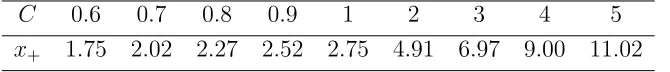
Table 1: B = 1
C 0.6 0.7 0.8 0.9 1 2 3 4 5
x+ 1.75 2.02 2.27 2.52 2.75 4.91 6.97 9.00 11.02
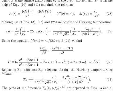
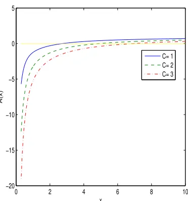
Figs. 1 and 2. According to Fig. 1 at m0 6= 0 (B = 1) there is only one
horizon. For the bigger mass (the parameterC is greater) the horizon radius increases. Figure 2 shows that there are no horizons at m0 = 0, B <3.17),
an extreme horizon occurs at m0 = 0, B ≈ 3.173, and two horizons hold at
m0 = 0 andB >3.173.
Making use of Eqs. (2) and (7) atE = 0, we obtain the Ricci scalar
R= 8πGTµµ= 16πGβq
4
m
(r4+βq2
m)2
. (26)
Table 2: m0 = 0
B 3.173 3.2 3.5 4 4.5 5 6 7 8
x− 1.68 1.52 1.21 1.03 0.92 0.85 0.75 0.68 0.63
x+ 1.68 1.87 2.49 3.19 3.82 4.42 5.59 6.74 7.87
5
The black hole thermodynamics
To study the black holes thermodynamics and the thermal stability of mag-netic BHs, we consider the Hawking temperature
TH =
κ
2π =
A0(r+)
4π , (27)
where κ is the surface gravity and r+ is the event horizon radius. With the
help of Eqs. (10) and (11) one finds the relations
A0(r) = 2GM(r)
r2 −
2GM0(r)
r , M
0
(r) =r2ρ, M(r+) =
r+
2G. (28)
Making use of Eqs. (3), (27) and (28) we obtain the Hawking temperature
TH = 1
4π
1
r+
−2Gr+ρ(r+)
!
= 1
4πβ1/4√q
m
1
x+
−√Gqmx+
β(1 +x4 +)
!
. (29)
Using the equation M(r+) =r+/(2G) and (21) we find
Gq√m
β =
4√2(x+−2C)
D ,
D≡lnx
2−√2x+ 1
x2+√2x+ 1 −2 arctan(1−
√
2x) + 2 arctan(1 +√2x). (30)
Replacing Eq. (30) into Eq. (29) one obtains the Hawking temperature as follows:
TH ==
1 4πβ1/4√q
m
1
x+
−4
√
2(x+−2C)x+
(1 +x4 +)D
. (31)
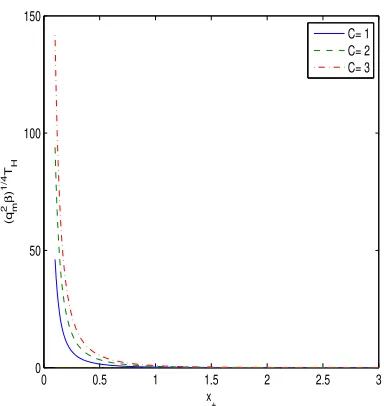
The plots of the functions TH(x+)
√
qmβ1/4 are depicted in Figs. 3 and 4.
0 2 4 6 8 10 −20
−15 −10 −5 0 5
x
A(x)
C= 1 C= 2 C= 3
Figure 1: The plot of the function A(x) for B = 1. The solid curve is for
C = 1, the dashed curve corresponds to C = 2, and the dashed-doted curve corresponds to C = 3.
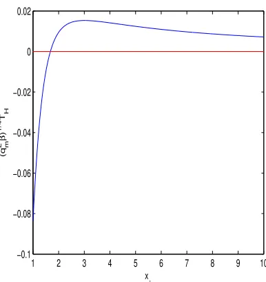
C 6= 0 (m0 6= 0). Figure 4 shows that the Hawking temperature for C = 0
(m0 = 0) is positive for x+ >1.679 and is zero at x+ ≈ 1.679 . The BH is
unstable when the temperature is negative. From Eq. (30) we obtain the value of Gqm/√β = 3.173 corresponding to x+ = 1.679. By studying the
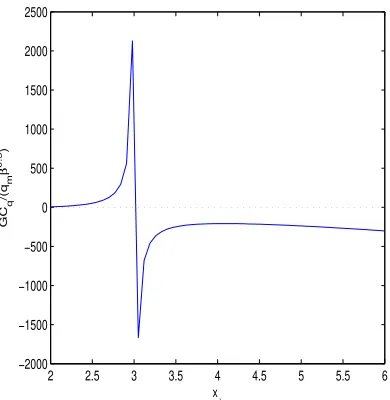
signs of the heat capacity and the Helmholtz free energy, we can observe the different stability phases of the BH [51]. Making use of the Hawking entropy of the BH S = Area/(4G) = πr+2/G = πx2+qm√β/G we find the heat capacity
Cq =TH
∂S
∂TH
!
q
= TH∂S/∂x+
∂TH/∂x+
= 2πqm
√
βx+TH
G∂TH/∂x+
. (32)
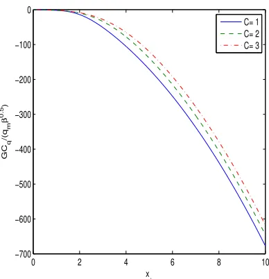
According to Eq. (32) the heat capacity possesses a singularity when the Hawking temperature has an extremum (∂TH/∂x+ = 0). The plots of the
heat capacity versus the variable x+ for different parameters C are depicted
in Figs. 5. 6, and 7. Figure 5 shows the Schwarzschild behaviour of the heat capacity for C 6= 0 (m0 6= 0), i.e. it is negative at ∂TH/∂x+ <0. As a
0 1 2 3 4 5 6 7 8 −0.6
−0.4 −0.2 0 0.2 0.4 0.6 0.8 1
x
A(x)
B= 2 B= 3.175 B= 5
Figure 2: The plot of the function A(x) for m0 = 0. The solid curve is for
B = 2, the dashed curve corresponds to B = 3.175, and the dashed-doted curve corresponds to B = 5.
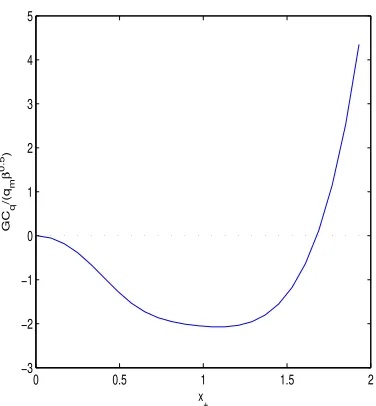
the BH is unstable at 1.679 > x > 0 because the heat capacity is negative. Figure 7 shows a singularity in the heat capacity at the point x ≈ 3 where the second-order phase transition occurs. When m0 = 0 the heat capacity is
positive at the range 3 > x >1.679 and the BH is stable.
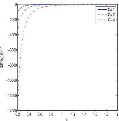
To complete the analysis of phase transitions we consider the Helmholtz free energy which is given by
F =m−THS. (33)
The mass of the BHm plays the role of the internal energy, and the Hawking entropy is S =πr2+/G. Making use of Eqs. (22). (31) and (33) we obtain
GF √
qmβ1/4
=B C+ π
4√2 !
−x+
4 +
√
2x2+(x+−2C)
(x4
++ 1)D
. (34)
Substituting B =qmG/ √
β from Eq. (30) into (34) we find
GF √
qmβ1/4
= C+ π
4√2 !
4√2(x+−2C)
D −
x+
4 +
√
2x2
+(x+−2C)
(x4
++ 1)D
0 0.5 1 1.5 2 2.5 3 0
50 100 150
x +
(q
m
2β
)
1/4
TH
C= 1 C= 2 C= 3
Figure 3: The plot of the function TH √
qmβ1/4 vs x+. The solid curve is for
C = 1, the dashed curve corresponds to C = 2, and the dashed-doted curve corresponds to C = 4.
The plots of the unitless reduced free energy GF/(√qmβ1/4) vs. x+ are
depicted in Figs. 8 and 9. The BHs with F > 0, Cq <0 are unstable and
the BHs with F <0, Cq >0 are stable. In accordance with Figs. 5-9, there
are other phases with F >0,Cq >0 and F <0, Cq <0. In the case F <0,
Cq < 0 the BHs are less energetic than the pure radiation and, as a result,
BHs do not decay through tunneling. For large masses of BHs (C >1) this phase holds. Because the heat capacities are negative, the BH temperature decreases when the mass of BH increases. Such phases are also realised in another model [52].
6
Conclusion
1 2 3 4 5 6 7 8 9 10 −0.1
−0.08 −0.06 −0.04 −0.02 0 0.02
x+
(q
m
2
β
)
1/4
TH
Figure 4: The plot of the function TH √
qmβ1/4 vs x+ for C= 0 (m0 = 0).
magnetic BHs in GR were studied. It was shown that in the self-dual case (qe =qm) the corrections to Coulomb’s law and RN solutions are absent. The
Ricci scalar does not have the singularity and asr → ∞space-time becomes flat.
The thermodynamics and the thermal stability of magnetized BHs were investigated. The Hawking temperature, the heat capacity and the Helmholtz free energy of BHs were calculated. It was demonstrated that the heat capac-ity diverges at some event radiir+ (x+) for the case when the total BH mass
is the magnetic mass and the phase transitions of the second-order occurs. We shown that there is a new stability region of BH solutions when the heat capacity and the free energy are negative. In this case BHs are less energetic than the pure radiation and BHs do not decay via tunneling.
References
[1] A. D. Shapere, S. Trivedi, and F. Wilczek, Mod. Phys. Lett. A 6, 2677 (1991).
0 2 4 6 8 10 −700
−600 −500 −400 −300 −200 −100 0
x +
GC
q
/(q
m
β
0.5
)
C= 1 C= 2 C= 3
Figure 5: The plot of the function GCq/(q2mβ)1/2 vs x+. The solid curve is
for C = 1, the dashed curve corresponds to C = 2, and the dashed-doted curve corresponds to C = 3.
[3] M. Cvetic and A. A. Tseytlin, Phys. Rev. D 53, 5619 (1996); Erratum: Phys. Rev. D 55, 3907 (1997).
[4] D. P. Jatkar, S. Mukherji, and S. Panda, Nucl. Phys. B484, 223 (1997). [5] A. H. Chamseddine and W. A. Sabra, Phys. Lett. B 485, 301 (2000). [6] D. D. K. Chow and G. Compere, Phys. Rev. D 89, 065003 (2014). [7] P. Meessen, T. Ortn, and P. F. Ramrez, JHEP 1710, 066 (2017). [8] H. Lu, Y. Pang, and C.N. Pope, JHEP 1311, 033 (2013).
[9] S. A. Hartnoll and P. Kovtun, Phys. Rev. D 76, 066001 (2007).
[10] S. A. Hartnoll, P. K. Kovtun , M. Muller, and S. Sachdev, Phys. Rev. B 76, 144502 (2007).
0 0.5 1 1.5 2 −3
−2 −1 0 1 2 3 4 5
x +
GC
q
/(q
m
β
0.5
)
Figure 6: The plot of the function GCq/(qm2β)1/2 vs x+ for C = 0.
[13] M. Born and L. Infeld, Proc. R. Soc. Lond. 144, 425 (1934). [14] W. Heisenberg and H. Euler, Z. Phys. 98, 714 (1936).
[15] H. H. Soleng, Phys. Rev. D 52, 6178 (1995).
[16] D. M. Gitman and A. E. Shabad, Eur. Phys. J. C 74, 3186 (2014). [17] C. V. Costa, D. M. Gitman, and A. E. Shabad, Phys. Scripta90, 074012
(2015).
[18] S. I. Kruglov, Commun. Theor. Phys. 66, 59 (2016). [19] S. I. Kruglov, Mod. Phys. Lett. A 32, 1750201 (2017).
[20] R. Pellicer and R. J. Torrence, J. Math. Phys. 10, 1718 (1969). [21] H. P. de Oliveira, Class. Quant. Grav. 11, 1469 (1994).
[22] E. Ay´on-Beato and A. Gar´cia, Phys. Rev. Lett. 80, 5056 (1998). [23] K. A. Bronnikov, V. N. Melnikov, G. N. Shikin, and K. P. Staniukovich,
2 2.5 3 3.5 4 4.5 5 5.5 6 −2000
−1500 −1000 −500 0 500 1000 1500 2000 2500
x
+
GC
q
/(q
m
β
0.5
)
Figure 7: The plot of the function GCq/(qm2β)1/2 vs x+ for C = 0.
[24] K. A. Bronnikov, Phys. Rev. D 63, 044005 (2001). [25] K. A. Bronnikov, Phys. Rev. Lett. 85, 4641 (2000).
[26] K. A. Bronnikov, G. N. Shikin, and E. N. Sibileva, Grav. Cosmol.9, 169 (2003).
[27] A. Burinskii and S. R. Hildebrandt, Phys. Rev. D 65, 104017 (2002). [28] J. Diaz-Alonso and D. Rubiera-Garcia, Phys. Rev. D81, 064021 (2010). [29] N. Breton, Gen. Rel. Grav. 37, 643 (2005).
[30] M. Novello, S. E. Perez Bergliaffa, and J. M. Salim, Class. Quant. Grav.
17, 3821 (2000).
[31] R. Garcia-Salcedo, T. Gonzalez, and I. Quiros, Phys. Rev. D89, 084047 (2014).
0.2 0.4 0.6 0.8 1 1.2 1.4 1.6 1.8 2 −14000
−12000 −10000 −8000 −6000 −4000 −2000 0
x +
GF/(q
m
2β
)
1/4
C= 1 C= 2 C= 4
Figure 8: The plot of the function GF/(√qmβ1/4) vs. x+. The dashed curve
corresponds to C = 2, the solid curve is for C = 1, and the dashed-doted curve corresponds to C = 4.
[34] S. I. Kruglov, Phys. Rev. D 94, 044026 (2016). [35] S. I. Kruglov, Ann. Phys. (Berlin) 528, 588 (2016).
[36] H. Yajima and T. Tamaki, Phys. Rev. D 63, 064007 (2001). [37] K. A. Bronnikov, Grav. Cosmol. 23, 343 (2017).
[38] K. A. Bronnikov, Int. J. Mod. Phys. D 27, 1841005 (2018). [39] S. I. Kruglov, Int. J. Mod. Phys. A 33, 1850023 (2018). [40] S. I. Kruglov, Ann. Phys. 383, 550 (2017).
[41] R. Garc´ıa-Salcedo and N. Breton, Int. J. Mod. Phys. A15, 4341 (2000). [42] C. S. Camara, M. R. de Garcia Maia, J. C. Carvalho, and J. A. S. Lima,
Phys. Rev. D 69, 123504 (2004).
[43] E. Elizalde, J. E. Lidsey, S. Nojiri, and S. D. Odintsov, Phys. Lett. B
0 0.5 1 1.5 2 −100
−80 −60 −40 −20 0 20 40 60
x +
GF/(q
m
2β
)
1/4
C= 0 C= 0.1 C= 0.2
Figure 9: The plot of the function GF/(√qmβ1/4 vs. x+). The dashed curve
corresponds to C = 0.1, the solid curve is for C = 0, and the dashed-doted curve corresponds to C = 0.2.
[44] M. Novello, S. E. Perez Bergliaffa, and J. M. Salim, Phys. Rev. D 69, 127301 (2004).
[45] M. Novello, E. Goulart, J. M. Salim, and S. E. Perez Bergliaffa, Class. Quant. Grav. 24, 3021 (2007).
[46] D. N. Vollick, Phys. Rev. D 78, 063524 (2008). [47] S. I. Kruglov, Phys. Rev. D 92, 123523 (2015).
[48] S. I. Kruglov, Int. J. Mod. Phys. A 32, 1750071 (2017). [49] S. I. Kruglov, Int. J. Mod. Phys. D 25, 1640002 (2016).
[50] A. E. Shabad and V. V. Usov, Phys. Rev. D 83, 105006 (2011).5). [51] S. W. Hawking and D. N. Page, Commun. Math. Phys. 87, 577 (1983). [52] J. A. R. Cembranos, A. Cruz-Dombriz, and J. Jarillo, Universe, 1, 412