Study of constitutive behavior of ferroelectrics via self-consistent modeling and neutron diffraction

Study of Constitutive Behavior of Ferroelectrics via

Self-Consistent Modeling and Neutron Diffraction

Thesis by

Seyed-Maziar Motahari

In Partial Fulfillment of the Requirements

For the Degree of

Doctor of Philosophy

California Institute of Technology

Pasadena, California

© 2007

Acknowledgments

Thanks first to my advisor and primary collaborator in this work, Professor Ersan Ustundag, for his support throughout my graduate studies. I’m grateful to Professor Kaushik Bhattacharya for acting as my Caltech advisor while I lived in Ames, Iowa. I am also very thankful to Professor Guruswami Ravichandran, Professor Chiara Daraio, and Professor Bill Johnson for participating in my defense as members of my committee.

I want to gratefully acknowledge the contributions of my research group mates: Dr. Seung-Yub Lee, Goknur Tutuncu, Mesut Varlioglu, Dr. Rob Rogan, Dr. Can

Aydiner, Dr. Jacob Jones, and Sarah Shiley. They have not only been instrumental in collecting data necessary to this thesis, they have also offered support and assistance in numerous other ways, not the least of which has been their friendship. Two former fellow Caltech students, Dr. Arash Yavari and Dr. Amir Sadjadpour, have provided counsel, insight, enthusiasm, and inspiration, for which I will be forever indebted.

Abstract

The central goal of this study is to develop a reliable self-consistent model to describe the constitutive behavior of polycrystalline ferroelectrics and to predict their lattice strain and texture evolution. Starting with the model developed by Huber et al. formulations and refinements were added to increase both the functionality and the accuracy of the model’s results. These refinements include methods for calculating lattice strain, tracking the number of domains contributing to diffraction patterns, locking the domain switching at a specified level, inputting initial grain orientation distribution, and a correction for a major flaw in the previous model: the phenomenon of reverse domain switching.

The comparison of model predictions and diffraction data from BaTiO3 yielded the following observations: (i) domain switching starts at very low stresses (< 10 MPa) and proceeds gradually; (ii) domains with c-axes closer to the loading axis start switching earlier and experience more switching; (iii) lattice-plane-specific (hkl) strains, with the exception of (111), exhibit apparent hardening after switching starts. The level of agreement between the model and the experimental data was

List of Illustrations

Figure 1-1: The perovskite crystal structure common to many ferroelectric ceramics. For BTO the white ions at the corners are Ba+2_{, the black ions on the faces are O}-2_, and the central ion is Ti+4. The top set of figures illustrates the phase change through the Curie temperature, the spontaneous polarization, and the linear response of the crystal. The bottom set of figures illustrates the spontaneous shape change of the crystal, and 180° and 90° switching due to applied electric field or stress. The magnitudes of the ion displacements have been exaggerated for clarity. (Courtesy of C. Landis [8])... 4

Figure 1-2: Plane view of a crystal aggregate with domains as subregions of equal spontaneous polarization after cooling below the Curie temperature... 6

Figure 1-3: At the paraelectric-ferroelectric phase transition of a material with tetragonal unit cell, there are six different directions for the central titanium ion to be displaced, resulting in six different spontaneous polarization vectors. ... 7

Figure 2-1: An ellipsoidal inclusion, I, is cut out of the matrix, M. ... 18

Figure 2-2: The inclusion has undergone a stress-free transformation, eigenstrain T, and has been placed back in the matrix. The matrix applies constraining traction forcing the inclusion to assume a final strain C, which can be related to T using the Eshelby tensor, S... 18

Figure 2-3: (a) The material properties of the inclusion are different from those of the matrix. The eigenstrain is real, due to a change in temperature, a phase

Figure 2-4: In the case of external loading, the total stress in the inclusion is the sum of the stress due to the mismatch of thermal coefficients or a phase transformation and the applied stress at infinity. Again, (a) depicts the real problem and (b) is the imaginary one... 21

Figure 2-5: Euler angles , , and can be used to define the orientation of any object in three-dimensional space by applying three consecutive rotations to an object lying along the x-axis in a Cartesian system of coordinates. (Illustration from

MathWorld.com)... 25

Figure 2-6: Calculated (lines) and measured (symbols) stress-strain response parallel to the tensile axis for stainless steel. The experimental and modeling results have a good match in the elastic region. The results are less agreeable in the plastic regime. (Courtesy of B. Clausen)... 31

Figure 3-1: The progressive nature of ferroelectric transformation within a crystal due to domain wall motion. This simplified example has only 2 domains, and the loading space is one-dimensional. (Courtesy of C. Landis) ... 35

Figure 3-2: Self-consistent model estimates of the electrical displacement (top) and the strain (bottom) responses of a ferroelectric polycrystal to cyclic electric field loading [8]... 38

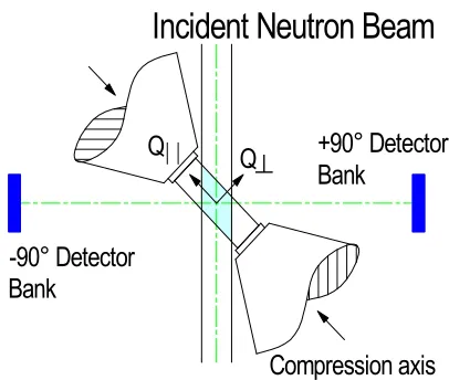
Figure 3-3: Schematic of the experimental setup at ENGIN X. The diffracted neutrons are collected by two 2θ = ±90º detectors with scattering vectors

corresponding to the longitudinal and transverse directions of the specimen. ... 40

Figure 3-4: The domain selection mechanism incorporated into the new model. The [002] direction in domain 1, the [200] direction in domain 2, the [103] direction in domain 5, and the [301] direction in domain 6 are perfectly aligned with the

contribute to the diffraction pattern. If these were the only grains in the material lattice strain [002] would be the average of the strains in domains 1 and 3, the strain along [200] would be the average of domains 2 and 4, the strain along [103] would be equal to the strain of domain number 5, and the strain along [301] would be equal to that of domain number 6... 41

Figure 3-5: Schematic of two domains in a grain. Domain A is along direction 1, and domain B is along direction 2. Transformation is defined as switching of A to B. Transformation ‘-’ would be switching of B to A... 43

Figure 3-6: Plot of Equation (3.21) - the driving force for transformation ‘ ’ versus. applied stress, 11. Whether 11 increases in tensile or in compressive directions, the transformation ‘ ’ will not take place. Instead the transformation ‘- ’ will occur, no matter what the sign of 11 is. Referring to Figure 3-5, it is clear that the

transformation ‘- ’ will be physically meaningless under this applied compressive stress... 45

Figure 3-7: Same as in Figure 3-6, except the relative value of Gc is smaller. As compressive stress along direction 1 is increased transformation ‘ ’ occurs as

expected. Increasing compressive 11 even further causes a transformation in the ‘- ’ direction, which is an unrealistic case... 45

Figure 4-1: A closer schematic of the sampling volume in Figure 3-3. Lattice planes and their d-spacings sampled by the longitudinal and transverse detectors are

highlighted. ... 50

Figure 4-2: Diffraction spectra from a time-of-flight neutron diffraction experiment at ENGIN X using an unloaded BaTiO3 polycrystal. The x-axis is either in terms of time-of-flight (a) or d-spacing (b), while the y-axis is the intensity of the diffracted neutrons in terms of counts per microsecond. ... 52

Figure 4-3: Single-peak fitting to reflections (200) and (002) of BaTiO3. ( a) Raw data and the fitted peak with peak position and intensity refined. (b) Peak width is added to the fitted parameters and a better fit is achieved (Rp = 3.5% , 2 = 1.2, where Rp is the minimum achievable pattern residual, and 2 is the chi-square goodness-of-fit)... 55

Figure 4-4: (a) A full-pattern Rietveld fit to the diffraction data from a BaTiO3

polycrystalline sample.(b) The (002) / (200) doublet shows a fit as good as that of the single-peak fitting method. This would not be the case when loading increases. ... 61

Figure 4-5: Different grains have different plane-specific elastic moduli, hence will exhibit different lattice strains. ... 64

Figure 4-6: Schematic definition of angles φ and ρ in hexagonal (left) and tetragonal (right) unit cells... 66

Figure 4-7: Crystallographic-direction-specific Young’s modulus (Ehkl) of beryllium (left) and magnesium (right) compared to approximations by Equations (4.20) and (4.22). The γi parameters in these equations were refined to obtain the best fit to the Ehkl curve... 68

Figure 5-1: (002)/(200) peaks of BaTiO3: (a) is the unloaded sample, and (b) is under –100 MPa compressive stress. The dots are raw data while the green lines are the Rietveld fits. The Rietveld method fails to capture the texture evolution as loading has increased. ... 72

Figure 5-2: At zero loading the March-Dollase (M-D) coefficient value is 1.0, which indicates a random grain distribution. As loading increases, the M-D value increases, indicating domain switching. The change starts at very small loads... 73

Figure 5-3: (002)/(200) doublet and single-peak fits to the data using two type 3 peak profiles in GSAS. Both samples are BaTiO3: (a) is a stress- free sample, and (b) is under a compressive stress of –100 MPa. Comparison to Figure 5-1 shows the

superiority of the single-peak method in texture analysis. ... 74

Figure 5-4: Peak Intensity Ratio diagrams for peak doublets (left to right) (200) / (002), (311) / (113), and (220) / (202). The independent axis is the y-axis which is the applied compressive stress in MPa. ... 76

Figure 5-5: Definition of angle α between the loading axis (no. 1) and the c-axis of the red domain as it transforms into the blue domain. The unit vectors n and s are defined as the inside and outside bisectors, respectively, between the domains’ c-axes. ... 77

Figure 5-6: Rietveld analyses of polycrystalline a BaTiO3 sample with different crystal structures. (a) Tetragonal under -5 MPa stress, (b) tetragonal and

orthorhombic under -5 MPa stress, (c) tetragonal under -220 MPa stress, and (d) tetragonal and orthorhombic under -220 MPa stress. ... 80

Figure 5-8: The evolution of (002) / (200) peak doublets under loading analyzed with the single-peak fitting method. As loading increases (0 MPa, 50 MPa, and 150 MPa), the (002) peak vanishes, making a single peak fit impossible or extremely erroneous. ... 83

Figure 5-9: Rietveld anisotropy parameter (γ in Equation (4.16)), a measure of the degree of anisotropy. Anisotropy increases as the sample is loaded. ... 84

Figure 5-10: Longitudinal lattice strains from neutron diffraction versus applied uniaxial compression of BaTiO3. The strain data were obtained from single-peak fitting. Linear trendlines were fitted to each data set to guide the eye. Note the extreme scatter in the (002) data due to diminished peak intensity at high applied stresses. ... 84

Figure 5-11: Sample BaTiO3 macrostrain (elastic plus permanent) along the loading direction measured by an extensometer versus applied compressive stress ... 85

Figure 5-12: Longitudinal lattice strains predicted by an elastic calculation of the SCM versus applied uniaxial compression of BaTiO3. The calculations employed the elastic constants listed in Table 5-1 and considered no domain switching. Note the relative slopes of the hkl-dependent lattice strains in comparison to the data on Figure 5-10. ... 86

Figure 5-14: Lattice strain evolution under applied stress predicted by the SCM for (a) the (200) / (002) doublet, and (b) the (311) / (113) doublet ... 90

Figure 5-15: (111), (200), and (002) lattice strains obtained from the new model are compared with diffraction data. (111) does not demonstrate nonlinearity, the other two crystal directions exhibit apparent hardening during switching in both

List of Tables

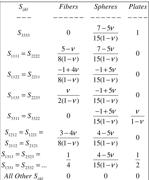
Table 2-1: Components of the Eshelby tensor. is the Poisson’s ratio of the infinite matrix. ... 19

Table 4-1: Initial values used as a starting point for Rietveld refinements in BaTiO3 experiments... 60

Table 5-1: Input data for the self-consistent program to model the BaTiO3 experiment. SE are the components of the elastic compliance tensor, d is the

Table of Contents

Acknowledgments...iii

Abstract... iv

List of Illustrations ... vi

List of Tables...xiii

Table of Contents ... xiv

1.

Introduction ...1

1.1 Ferroelectric Materials: Definition and Application... 1

1.2 Piezoelectricity: Governing Equations... 9

1.3 Ferroelectrics: Constitutive Modeling... 12

1.4 Goal and Outline of Thesis... 14

2.

The Self-Consistent Model...17

2.1 The Eshelby Tensor... 17

2.2 Inhomogeneous Inclusion ... 19

2.3 Multiple Inclusions... 22

2.4 Polycrystals and the Self-Consistent Model ... 23

3.1 The Huber Model ... 32

3.2 The New Self-Consistent Model... 39

3.2.1 Grain Selection and Average Lattice (hkl) Strain ... 39

3.2.2 The Problem of Reverse Switching... 42

4.

Neutron Diffraction Experiments ...49

4.1 Introduction ... 49

4.2 Experimental Setup and Sample Properties ... 50

4.3 Calculating Lattice Strains: the Single-Peak Method ... 53

4.4 Calculating Lattice Strains: the Rietveld Method ... 56

4.5 Calculating Lattice Strains: the Improved Rietveld Method .. 63

5.

Conclusions and Future Work ...71

5.1 Experimental Conclusions: Texture Evolution... 71

5.2 Experimental Conclusions: Lattice Strains ... 81

5.3 Modeling Conclusions... 87

5.4 Summary and Conclusions... 93

5.5 Future Work ... 95

1.

Introduction

1.1 Ferroelectric Materials: Definition and Application

Nowadays, many engineering problems necessitate the implementation of “smart”, i.e., adaptive or controlled, systems. Since these systems usually possess both sensing and actuation capabilities, a variety of physical phenomena are often coupled for their technical implementation. Thermal expansion, shape memory effect,

magnetostriction, electrostriction, and piezoelectricity are some important examples of such coupling phenomena. It is now a matter of technical needs and costs that determine which coupling mechanism and which material will be the best choice.

Piezoceramics are outstanding candidates for mass applications calling for short response times, high-precision positioning and considerable actuation forces in systems of possibly complex shape. In this thesis, the term piezoceramic denotes polycrystalline ferroelectric materials (in general, they are ferroelastic as well) used for the exploitation of piezoelectricity in engineering. Barium titatnate (BaTiO3) and lead zirconate titanate (PZT) are the most prominent materials in this class. While the former is the favored model material in fundamental material science investigations, the latter is preferred in technical applications due to its optimum electromechanical coupling properties [1].

ferroelectrics originates from their large electromechanical coupling and their ability to be easily manufactured into complex geometries via powder processing and other advanced fabrication techniques. The phenomena of ferroelectricity, ferroelasticity, and piezoelectricity are here presented with reference to the commonly found perovskite crystal structure [3]. What will become clear in this discussion is that the unusual electromechanical macroscopic properties found in these materials can only be understood through an appreciation of the physical mechanisms operating in a multiaxial fashion at a range of microstructure-dependent length scales. The

interaction of anisotropic mechanisms at multiple length scales leads to complicated behavior dependent on the specific application of external forces and the

microstructure of the specimen under investigation.

A ferroelectric material is a piezoelectric material with the ability to switch its polarization direction under an applied electric or mechanical field. The microscopic structure of piezoelectric materials is crystalline in nature. In a crystalline material, the crystal lattice is a periodical repetition of a unit cell. A ceramic material is divided into grains with differing orientations of the crystal lattice. The unit cell consists of a buildup of positively and negatively charged ions typical of a specific material. According to this buildup, the centers of the positive and negative charges of the unit cell possess specific locations within the cell.

to be polarizable if the centers can be shifted with respect to one another by the application of an external load, leading to a load-induced dipole in the unit cell. In the case of electric loading, the load is the applied electric field.

If the centers of positive and negative charge are at different positions from one another within the unit cell, even in the absence of any load, then the cell is considered to possess spontaneous polarization. In other words, the unit cell has a permanent dipole. In such a case, the material is called a polar material.

Mathematically, any relative displacement of the centers of positive and negative charge in a unit cell is described by the polarization vector. The magnitude of this vector is proportional to the distance between the centers and the respective sum of the positive and negative ionic charges. Polarization is usually denoted by P.

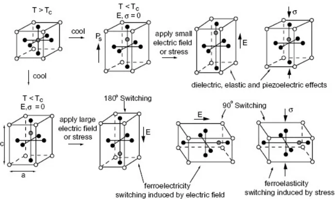
Figure 1-1 illustrates the perovskite structure for many ferroelectrics including BaTiO₃ (BTO) and Pb(Zr_xTi_1-x)O₃ (PZT). Here, only the tetragonal structure is discussed, however orthorhombic, rhombohedral, and monoclinic crystal structures are also known to exist in these materials [3-7]. Above the Curie temperature T

c, the

material is paraelectric with a cubic, centro-symmetric structure. As it is cooled below

T

c it undergoes a phase transformation from the cubic to tetragonal phase. Notice that

the previously centered Ti ion has been displaced towards one face of the tetragonal cell. The direction of this ion displacement is also the direction of the spontaneous polarization of the material, P

s, and is aligned with the c-axis of the tetragonal cell

ferroelectric, and the piezoelectric properties of the crystal are aligned with the spontaneous polarization direction. Rhombohedral phase ferroelectrics possess ion displacements and polarizations along the <111> cubic direction, and orthorhombic ones along the <110>.

Figure 1-1: The perovskite crystal structure common to many ferroelectric ceramics. For BTO the white ions at the corners are Ba+2_{, the black ions on the faces are O}-2_{, and the}

central ion is Ti+4_{. The top set of figures illustrates the phase change through the Curie}

temperature, the spontaneous polarization, and the linear response of the crystal. The bottom set of figures illustrates the spontaneous shape change of the crystal, and 180° and 90° switching due to applied electric field or stress. The magnitudes of the ion displacements

have been exaggerated for clarity. (Courtesy of C. Landis [8])

strain will decrease (elastic effect) and the polarization will decrease (piezoelectric effect).

The ferroelectric response of the material is illustrated on the second row of Figure 1-1 where ferroelastic switching has been differentiated from ferroelectric switching [3]. Note that a change in spontaneous strain, i.e., the orientation of the c-axis, accompanies the polarization change during 90° switching but not during 180°

switching. For the tetragonal structure shown in Figure 1-1 there are four possible 90° switches that can be driven by combinations of stress and electric field, and one 180° switch that can be driven only by electric field. The middle two schematics on the second row of Figure 1-1 illustrate 180° and 90° switching induced by applied

electric field alone. The last schematic illustrates 90° switching due to the application of a compressive stress parallel to the polarization direction. Note that for this

compressive stress a switch to any one of the four energetically equivalent 90° domain variants can be activated.

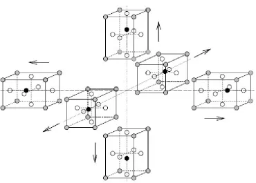
Across a domain wall the spontaneous polarization is discontinuous. Switching of a domain is not a homogenous process as the single unit cell depiction would suggest, but rather proceeds as a result of domain wall motion which converts one domain variant to another [3, 5, 6, 9]. Even within a single crystal different concentrations of the six possible domain variants can coexist such that the irreversible (or remanent) polarization, and hence the piezoelectric properties, of the crystal can be oriented in any of these six directions through application of a large electric field to induce domain switching; this process is called “poling.” The ability of ferroelectric single crystals to be poled in certain directions is of significant technological importance, as it allows for the piezoelectric response to be oriented for use in applications.

Successful poling of a single crystal depends on the relative concentrations of the initial domain variants, crystal purity (any impurities can impede domain wall motion), and the direction and strength of the applied electric field.

.

Figure 1-3: At the paraelectric-ferroelectric phase transition of a material with tetragonal unit cell, there are six different directions for the central titanium ion to be displaced,

resulting in six different spontaneous polarization vectors.

initially homogenous orientation distribution of the ceramic implies that the specimen may be poled in an arbitrary direction.

As the electric field is applied, domain walls move such that domains aligned with the field grow at the expense of domains opposing the field. However, the randomized grain and domain configuration established during preparation limits the possible orientations of any domain variant relative to the externally applied field. Thus, during poling, domains will attempt to switch their polarizations into orientations aligned with the macroscopic field, but the fixed grain structure may severely limit switching ability [2]. The poling process, then, occurs gradually and over a range of applied electric fields due to the variation in local electromechanical boundary conditions (intergranular constraints). In certain grain orientations, domains may switch temporarily to minimize the total energy during the application of an electric field. After the field is removed, some domain walls will move back towards their original positions, due to residual stresses and local electric fields in the material. However, this reverse switching is incomplete and there exists a net polarization, strain and piezoelectric effect aligned in the direction of the original applied electric field. The material is now “poled” and suitable for use as an actuator or sensor.

Many of the most industrially successful ferroelectric compositions possess grains of multiple crystal structures, such as the rhombohedral-tetragonal phase combination found in the morphotropic region of the PZT phase diagram [5]. As such,

mechanical loads which produce large internal stresses that eventually lead to failure. Efforts to model and predict the behavior of ferroelectrics have often been hindered by the lack of suitable constitutive relations that accurately describe the

electromechanical response of these materials. While many measurements have been conducted on the macroscopic response of large single crystals or polycrystals, there is lack of multiaxial (and multiscale) data about the in-situ internal strain and texture response of these materials; this information is critical to the development of accurate models, and it can only be provided by diffraction techniques which directly measure internal lattice strains and crystallographic orientations. This thesis will present a comparison of a mechanics model with diffraction data.

1.2 Piezoelectricity: Governing Equations

In a ferroelectric, domain wall motion within each crystal leads to a change in the remanent strain and polarization. This non-linear switching closely resembles plastic deformation by slip in a metallic polycrystal: domain wall motion can be treated in an analogous manner as dislocation slip in elastic-plastic crystals.

Consider an anisotropic ferroelectric solid subjected to an electric field Ei and to a

mechanical stress ij. By assigning the notation superscript ‘L’ for the recoverable

(assumed linear) part and the superscript ‘R’ for the remanent part (equivalent to the plastic part in crystalline plasticity), one can decompose the total strain ij and the

j i ij

t

=

n

σ

and the surface-free charge density Q is in equilibrium with the jump in electric displacement <Di> across S, such that

(

)

i i i i i

Q n

= <

D

>=

n D

−

D

Here, the symbol “<>” to denotes the jump in a quantity at the boundary and o i D is the electrical displacement exterior to the body [8].

1.3 Ferroelectrics: Constitutive Modeling

1.3.1 Background

A successful design for a component in many engineering applications often

necessitates a complex interactive process that utilizes modeling and experimentation. This is especially crucial in predicting device/component performance and lifetime. To achieve this, it is essential that the model employs a realistic constitutive law that accurately describes material response to external loading.

One of the commonly used models is the Finite Element Method (FEM). In order to have an informative and detailed FEM model, one often needs to know the spatial distribution of the grains being modeled. This information is not readily available most of the time.

interact with an imaginary media (matrix) with properties derived from the average properties of all other grains. The self-consistent method has been used successfully in crystal elastoplasticity. It has also been used to predict the macroscopic behavior of ferroelectrics. The present study will show how it can be used for the investigation of lattice strains and texture evolution in ferroelectrics and how the results compare with neutron diffraction experiments.

The fundamentals of the self-consistent method are based on Eshelby’s inclusion method. In his papers published in 1957 and 1961, Eshelby [10, 11] solved the problem in closed form of an ellipsoidal inclusion in an infinite matrix with a misfit due to change in temperature. His approach can readily be expanded to solve the general problems of multiple inclusions, a finite matrix, and applied mechanical loading. Eshelby’s method and the aforementioned extensions are explained in Chapter 2. The Eshelby method has been further developed into a self-consistent method to solve polycrystalline plasticity problems. Studies have been conducted to simulate the development of lattice strain and texture during loading. These, too, will be briefly reviewed in Chapter 2.

1.3.2 Self-Consistent Modeling of Ferroelectrics

In their 1999 paper, Huber et al. developed an SCM to study macroscopic behavior of ferroelectrics [8]. Their model is based on the switching of differently oriented

macroscopic features of ferroelectric switching, but it lacks the capacity to compute lattice strains. The improvement of the model to obtain this capability is the subject of Chapter 4.

The work of Hall et al., 2005-2007 [12-15], seems, at first glance, to be similar to the present study. They have also studied lattice strains in ferroelectrics via physical experimentation and a micromechanical model. However, there are two major differences. They have conducted X-ray experiments to calculate lattice strains in PZT, but the experiments were not in situ. Instead, they measured residual lattice strains after the application and removal of an electric field. Then they rotated the sample around an axis perpendicular to the polarization axis and diffraction vector. The purpose of the experiments discussed in this thesis is to study the evolution of lattice strains while the loading is being applied. The second key difference is in the modeling. Due to the different nature of their experiments, they have been able to use a simple model which helps them explain why the lattice strain can be fitted linearly with moderate success using the cosine square of the rotation angle as the

independent variable. In comparison, the model presented here aims to predict the lattice strains given the single crystal properties of the ferroelectric and known domain switching criteria.

1.4 Goal and Outline of Thesis

neutron diffraction data. Along the way, it will be shown that improvements were needed in both the analysis of diffraction data and the self-consistent modeling.

The introduction to ferroelectrics, previous studies, and equations governing

ferroelectrics were explained in this chapter. Chapter 2 will discuss the self-consistent model and its basis, the Eshelby method, as they existed before the SCM was

extended into ferroelectrics. Cases of mechanical versus thermal loading, and single versus multiple inclusions are also discussed. Next, the formulation of SCM as a means to simulate grain-to-grain interactions is presented. Chapter 3 will explain the SCM for ferroelectric domain switching and the improvements made to a previous model to be able to compare its predictions with diffraction data.

Chapter 4 will elaborate on the experimental methods used and the experimental challenges faced. The single peak fitting and the multi-peak Rietveld method and their advantages and disadvantages will be discussed. Also, an improved version of the Rietveld method which should be used with anisotropic materials will be

discussed. This method is currently implemented in the common Rietveld code GSAS (General Structure Analysis System)[16] for some crystal structures. Guidelines on how to implement it for other structures are also provided in this chapter.

2.

The Self-Consistent Model

2.1 The Eshelby Tensor

The fundamentals of the self-consistent model are based on Eshelby’s inclusion method. In his papers published in 1957 and 1961, Eshelby [10, 11] solved the

problem of an ellipsoidal inclusion in an infinite matrix with a misfit due to change in temperature in closed form. His approach can readily be expanded to solve the

general problems of multiple inclusions, a finite matrix, and applied mechanical loading.

Assume an infinite media, referred to as ‘the Matrix.’ A part of the matrix is cut out, referred to as ‘the Inclusion,’ and undergoes a stress free transformation, or

‘eigenstrain.’ This eigenstrain can be due to a mismatch in thermal expansion coefficients, or it can be a result of a martensitic phase transformation, etc.

If the inclusion is to be put back in the matrix (Figures 2-1 and 2-2), due to the

known, which in this case is the same as the stiffness tensor for the inclusion, the residual strain and stress can be readily calculated:

C = S T (2.1)

I = CM ( C- T) = CM (S-U) T. (2.2)

The subscript Idenotes the inclusion and U in the equation is the identity matrix. Superscript C denotes a constrained value. T is the eigenstrain, and S is the Eshelby tensor.

++

Cut

M M _I

Figure 2-1: An ellipsoidal inclusion, I, is cut out of the matrix, M.

T _{Put back in}

C

I I

Figure 2-2: The inclusion has undergone a stress-free transformation, eigenstrain T_{, and has}

be applied to it. It can be shown that one can choose a size for the ghost inclusion and assume an eigenstrain for it such that the final constrained strain and the traction on the ghost inclusion are equal to the constrained strain and traction on the inclusion in the real problem. The conclusion is that the matrix is practically dealing with the same inclusion in cases (a) and (b), so the results can be used interchangeably.

T*

-->

M

(a)

(b)

T

-->

M

M

I

Figure 2-3: (a) The material properties of the inclusion are different from those of the matrix. The eigenstrain is real, due to a change in temperature, a phase transformation, etc. (b) The equivalent imaginary problem, constructed with an inclusion and a matrix that have the same

material properties so that the Eshelby formula can be applied

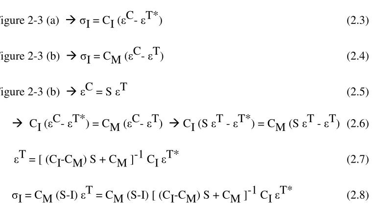
Figure 2-3 (a) I = CI ( C- T*) (2.3)

Figure 2-3 (b) I = CM ( C- T) (2.4)

Figure 2-3 (b) C = S T (2.5)

CI ( C- T*) = CM ( C- T) CI (S T - T*) = CM (S T - T) (2.6)

T = [ (CI-CM) S + CM ]-1 CI T* (2.7)

I = CM (S-I) T = CM (S-I) [ (CI-CM) S + CM ]-1 CI T* (2.8)

transformations, and T is the eigenstrain in the ghost inclusion which is just an imaginary construct.

Exactly the same concepts hold in the case of an applied external load (Figures 2-4a and 2-4b), only more care should be taken in writing the inclusion stress-elastic strain relationships. It is then possible to calculate the stress and constrained strain for such a case as well.

0 --> C₊ A

M

(a) (b)

T _--> C₊ A M

M

I

A

A A

Figure 2-4: In the case of external loading, the total stress in the inclusion is the sum of the stress due to the mismatch of thermal coefficients or a phase transformation and the applied

stress at infinity. Again, (a) depicts the real problem and (b) is the imaginary one.

(a) I + A = CI ( C + A) (2.9)

(b) I + A = CM ( C + A - T) (2.10)

(b) C = S T (2.11)

T = -[ (CI-CM) S + CM ]-1 (CI-CM) A (2.12)

I + A = -CM (S-I) [ (CI-CM) S + CM ]-1 (CI-CM) A + CM A (2.13)

In the above equations, A = CM A. Note that in this case Iis not the total inclusion

2.3 Multiple Inclusions

A single inclusion in an infinite matrix is not a very realistic situation, but instead multiple inclusions are usually present. One way to relate such a case to the calculations presented up to now is to assume that an inclusion does not have the whole matrix constraining it, but only a portion of the matrix around itself. As a result there would be less constraint and the inclusion will be more relaxed. One way to model this is to assume a background stress already present in the matrix denoted by < >M. The equations would now be very similar to what was presented before, for both external stress and eigenstrain. In case of eigenstrain:

I + < >M = CI ( C + < >M - T*) (2.14)

I + < >M = CM ( C + < >M - T) (2.15)

C = S T (2.16)

where , < >M = CM < >M is the background stress, and < >I I + < >M is the inclusion stress.

The value of the background stress should be such that the inclusion and matrix are in equilibrium. Thus:

f < >I + (1-f)< >M = 0 (2.17)

T = {(CM – CI)[S – f (S–I)] – CM}-1 CI T*. (2.18) From which stress in ‘M’ and ‘I’ can be calculated:

< >M = -f CM (S–I) T (2.19)

< >I = (1-f) CM (S–I) T. (2.20)

In the case of external loading the only difference would be T:

T = {(CM – CI)[S – f (S–I)] – CM}-1 (CM-CI) A (2.21)

and, of course, A should be added to obtain the total stress.

2.4 Polycrystals and the Self-Consistent Model

Almost all structural materials are polycrystals made up of multiple grains. In order to design and optimize engineering components constructed out of these materials, it is necessary to know the internal stress/strain state in the polycrystal.

Micromechanical polycrystal deformation models that are based on the deformation of the individual grains can be used to determine the overall stress state of a

e.g., Taylor 1938 [19], where all the grains are subjected to the same strain. These models do not account for anisotropy; hence, they do not serve our purposes.

A self-consistent model is one way of modeling grain-to-grain interactions. Similar to the Sachs and Hill methods, the topological aspects of the microstructure are

neglected in this method; instead, each grain interacts with other grains through the matrix, also called the homogeneous equivalent medium (HEM). The material properties of this matrix are an average of the properties of the grains that make up the conglomerate.

In the self-consistent model, the effects of elastic anisotropy can be considered. Most of the ferroelectric materials of interest are extremely anisotropic; thus, the self-consistent model provides a far superior method of analysis to the Sachs and Taylor models. In the rest of this section, details regarding the formulation of a

self-consistent method for solving problems of elastoplastic polycrystalline deformations are presented. These will serve as a useful guidance and background for the SCM of ferroelectrics presented in Chapter 3.

orientation of an object lying along the x-axis in a Cartesian coordinate system x-y-z by using these angles that represent three consecutive rotations. The first rotation is in the positive direction around the z-axis, the second is a rotation of around the new x-axis, and the third is a rotation of around the new z-axis.

Figure 2-5: Euler angles , , and can be used to define the orientation of any object in three-dimensional space by applying three consecutive rotations to an object lying along the

x-axis in a Cartesian system of coordinates. (Illustration from MathWorld.com)

The self-consistent model to be discussed here [20] is restricted to low strains, as the strain definition does not include second-order terms, and the model does not include localization, which can lead to instabilities such as necking. As a rule, a small strain model is valid as long as the tangent modulus is much larger than any of the stress components.

In their 1998 study [21], Clausen et al. examined the lattice strain development of three fcc materials (copper, aluminum, and steel) under uniaxial tension. They used Hutchinson’s self-consistent model [22] for elastic-plastic materials, as described in detail in this chapter. The model is a 1-site rate-insensitive SCM. Since all the materials studied are fcc, the slip systems contributing to plasticity are {111} <110>. The critical resolved shear stress (CRSS) obeys the hardening rule outlined earlier in this chapter in which three hardening parameters and the initial CRSS ( 0) are used as

fitting parameters to fit the macroscopic strain data.

Lattice strains were also calculated by the model are plotted versus applied stress. In the elastic regime, the lattice strains indicated more anisotropy in stainless steel than in copper, while the least elastic anisotropy was observed in aluminum. This is the expected result since the elastic anisotropy factor 2C44/(C11-C22) is highest in stainless

steel and lowest in aluminum.

The levels of anisotropy observed in the plastic regime were much larger than those in the elastic regime for all three materials. The 200 reflection showed the most unstable behavior, which also conforms to the ferroelectric data presented in Chapters 4 and 5.

elastic regime match very well. In the plastic regime, matching is good for some hkl and not particularly satisfactory for others. However, the model was judged capable of providing good qualitative predictions. Considering the complex nature of plastic-deformation and the non-topological micromechanical nature of the model, this can be considered a successful result.

Although Clausen et al. did not explore the phenomenon at that time, predictions of texture development can also be made using this model by plotting the number of active slip systems on each subset of grains. They focused instead on the number of grains that contain a specific number of active slip systems. Most of the activity occurs during the first stages of plastic deformation, after which the numbers remain more or less constant.

Clausen’s group also compared different lattice strains versus applied stress curves, and concluded that reflection 331 is a suitable one for stress-strain characterization, since it exhibits the most nearly linear response.

Figure 2-6: Calculated (lines) and measured (symbols) stress-strain response parallel to the tensile axis for stainless steel. The experimental and modeling results have a good match in

3.

Self-Consistent Modeling of

Ferroelectrics

3.1 The Huber Model

The starting point of the modeling effort in this study is the model developed by Huber et al. [8] which uses domain wall motion as the basis of a

microelectromechanical model. Domains are regions in which the spontaneous polarization and strain are homogenous and are separated from each other within a single crystal by mobile walls.

The basic equations governing the physical behavior of ferroelectrics were presented in Chapter 1. This section presents the assumptions in the model and how it can predict macroscopic behavior of ferroelectrics.

Grains (crystals) in this model interact via the self-consistent scheme, i.e., each grain only interacts with the homogenous matrix it is surrounded by. The matrix obtains its properties as a self-consistent average of properties of different grains.

angles also define their direction with respect to the global axes, or the laboratory coordinate system.

Currently the model considers a perovskite-type, tetragonal, single-phase material. The material has a cubic unit cell above the Curie temperature, but below that temperature (e.g., at room temperature) it has a tetragonal unit cell with the center of positive and negative ionic charges not coinciding, hence resulting in an electrical dipole in the unit cell.

Each grain has six energetically equivalent variants (domains) in three perpendicular directions (I=1 to 6). Each of the six variants can transform (switch) to any other five variants. Consequently thirty transformation systems are present ( =1 to 30).

The model also assumes that stress ( ) and electric field (E) in each variant are constant (i.e., the same) within a given grain. Strain ( ) and electric displacement (D) of the grain are taken to be the volume average of L and DL over the variants, plus the remnant strain and polarization due to switching.

Linear response ( L and DL) in each variant can be related to the action ( and E) on the variant (which is the same as the action on the grain) by the following equation:

=

E

d

d

S

D

I I L

L

σ

κ

ε

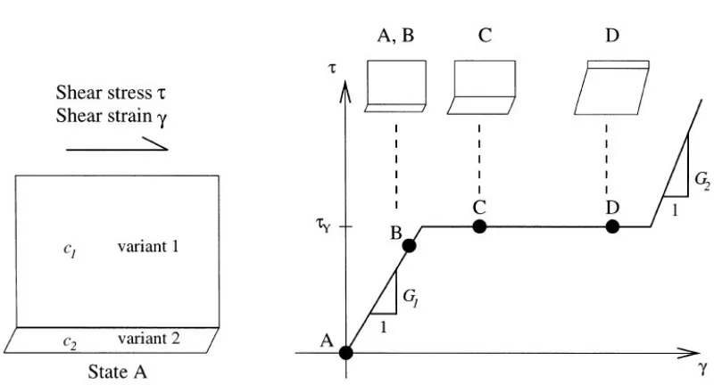
to one another, or switching occurs. A schematic of domain switching is illustrated in Figure 3-1. Here, the grain is assumed to have only two domains (variants), and the loading space has only one component: the shear stress.

Figure 3-1: The progressive nature of ferroelectric transformation within a crystal due to domain wall motion. This simplified example has only 2 domains, and the loading space is

one-dimensional. (Courtesy of C. Landis)

The challenge for ferroelectrics is to find the shape of the driving force function. If the loading were in the form of stress only, classical theories, such as von Mises could be used to combine different components of the stress tensor. But in

ferroelectrics there exist not only six stress components, but also three components of the electric field vector. Domain walls move when the driving force on the

corresponding transformation, G , reaches a critical value, Gc . The driving force is

defined as the work conjugate of the rate of transformation,fα, which are kinematic

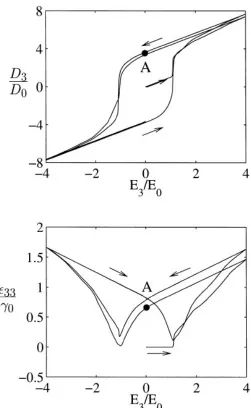
Figure 3-2: Self-consistent model estimates of the electrical displacement (top) and the strain (bottom) responses of a ferroelectric polycrystal to cyclic electric field loading [8]

3.2 The New Self-Consistent Model

3.2.1 Grain Selection and Average Lattice (hkl) Strain

The diffraction data include lattice plane spacings (d-spacings) yielding

hkl-dependent lattice strain evolution under loading. To study hkl-hkl-dependent properties of the material, the domains (or grains in general) which satisfy the Bragg’s law – the diffraction condition (i.e., those that will contribute to the diffraction pattern) should be selected and averaged over. This capability was incorporated into the new model.

To select the domains contributing to a specific reflection, the hkl vector (i.e., the lattice plane normal) of the domain should lie within a certain solid angle cone of the scattering vector of a given detector. The reason is that a detector in a diffraction experiment usually collects the diffracted beam through a solid angle cone called the acceptance angle. The value of the acceptance angle changes from detector to

⊥



Figure 3-3: Schematic of the experimental setup at ENGIN X. The diffracted neutrons are collected by two 2θ = ±90º detectors with scattering vectors corresponding to the

longitudinal and transverse directions of the specimen.

Figure 3-4 shows the mechanism of selecting domains that contribute to a given reflection. The new model identifies domains that have their hkl plane normal within the acceptance angle of a detector. The number of domains identified this way is counted such that each unit of 1/6th _{of a grain volume is counted as a single domain. It}

new model. This mechanism assures that even if the driving force on a specific transformation is more than the critical value resulting in all the domains to move out of a specific hkl direction, the transformation will not be activated. This way, there will always be domains that satisfy the diffraction condition and contribute to a reflection. While this “domain-locking” mechanism is somewhat artificial, it assures the presence of diffraction peaks throughout a loading experiment, a consistent fact in all diffraction data. The percentage of the domains which cannot be switched can be specified as a variable parameter in the program. The present study usually assumed 10% of the initially present domains will be locked (unless it is stated otherwise).

Another capability added to the new model is the ability to define texture. The original Huber model had the grains oriented along uniformly distributed directions. In the new model, one can define any texture at the beginning of the analysis.

3.2.2 The Problem of Reverse Switching

It was noticed that under certain conditions, i.e., low Gc values (Equation (3.17)),

domains that switched earlier under mechanical loading would tend to switch back using the original Huber model. The following describes the origin of this problem and the solution offered in the new model. The applied force space has nine

components: six stress components ( 11, 22, 33, 12, 13, and 23), and three electric

field components (E1, E2, and E3). To find out the shape of the driving force function

Defining transformation “

α

1

0 0

2

1

0 0

2

0 0 0

ij

µ

=

Note that I ijkl kl ij

s

σ σ

1

B A

A α _{= −}A α _{= . Hence one obtains:}

(

)

11 11

2 2

A B

s s

Gα = −γ σα − − σ . (3.21)

For an isotropic material Gαwill reduce to Gα = −γ σα 11/ 2, which is a linear

function of applied stress, while for an anisotropic material, Equation (3.21) is

quadratic. Based on the value of the critical driving force, Gc two different cases are

Gcr

-Gcr

Figure 3-6: Plot of Equation (3.21) - the driving force for transformation ‘ ’ versus. applied stress, 11. Whether 11 increases in tensile or in compressive directions, the transformation

‘ ’ will not take place. Instead the transformation ‘- ’ will occur, no matter what the sign of

11 is. Referring to Figure 3-5, it is clear that the transformation ‘- ’ will be physically

meaningless under this applied compressive stress.

Gcr

-Gcr

Figure 3-7: Same as in Figure 3-6, except the relative value of Gc is smaller. As

compressive stress along direction 1 is increased transformation ‘ ’ occurs as expected. Increasing compressive 11 even further causes a transformation in the ‘- ’ direction, which

is an unrealistic case.

In the first case (Figure 3-6), regardless of the sign of the applied stress

σ

4.

Neutron Diffraction Experiments

4.1 Introduction

Neutron diffraction is an ideal probe of bulk crystallographic structure, but so far in the realm of ferroelectrics, studies have mostly concentrated on probing the

temperature-composition-structure relationship to obtain a clear understanding of the nature of the various phase transitions [25]. Recently, some studies have begun to use neutrons for monitoring texture development in ferroelectrics using specimens

manipulated ex situ [12-15, 26]. Rogan et al. [25] have reported on the first in-situ bulk crystallographic study of the ferroelastic behavior of a multiphase,

polycrystalline PZT under compressive loading. The present thesis, however, investigates the behavior of single phase tetragonal BaTiO3. This material was largely chosen as a model system (its single crystal stiffness tensor is known in contrast to that of PZT), but it also exhibits useful piezoelectric properties.

Cylindrical bars of polycrystalline BaTiO3 were placed under uniaxial compression up to –300 MPa. Samples were oriented at a Bragg angle of

θ

θ

transverse sample response. In this thesis, all results and references are related to the longitudinal direction unless stated otherwise. In this case the scattering vector and the loading axis will always be parallel, so they will sometimes be referred to

interchangeably. Hot-pressed BaTiO3 was obtained from Alpha Ceramics Inc., (5121 Winnetka Avenue North, Minneapolis, MN 55428, USA). The BaTiO3 of grade EC-31 was obtained in bulk form in the unpoled state and diced using a diamond wafering saw to produce specimen of 6 x 6 x 14 mm. The samples were separated from the loading fixture using 7 x 7 x 4 mm stainless steel spacers.

Lattice (d-) spacings are related to the neutron wavelength, , and hence the time-of– flight (TOF), through the Bragg’ s law:

2 sin

n

λ

=

d

θ

Since the spallation (or TOF) neutron diffraction employed here generates a polychromatic beam, this equation means that multiple d-spacings are measured simultaneously while the Bragg angle (

θ

GSAS analysis software [16]. Additional details on data analysis of TOF neutron

200

002

200

002

Figure 4-3: Single-peak fitting to reflections (200) and (002) of BaTiO3. ( a) Raw data and

the fitted peak with peak position and intensity refined. (b) Peak width is added to the fitted parameters and a better fit is achieved (Rp = 3.5% , 2 = 1.2, where Rp is the minimum

4.4 Calculating Lattice Strains: the Rietveld Method

The Rietveld method uses a least-squares approach to refine a theoretical crystallographic model until it matches the measured diffraction pattern. The

introduction of this technique was a significant step forward in the diffraction analysis of powder samples as, unlike other techniques at that time, it was able to deal reliably with strongly overlapping reflections. The method was first reported [32] for the diffraction of monochromatic neutrons. The technique is equally applicable to alternative diffraction techniques such as x-rays or spallation (TOF) neutrons.

In the Rietveld method, least-squares refinements are carried out until the best fit is obtained between the entire observed powder diffraction pattern and the entire calculated pattern based on simultaneously refined models for crystal structure(s), instrumental factors, and other specimen characteristics such as lattice parameters. Some advantages of a full-pattern analysis (as compared to single-peak analysis) include [29]:

1. All reflections in the pattern are included without considering overlap. 2. The background is better defined, since a continuous function is fitted to the

whole pattern.

3. The effects of preferred orientation and extinction are reduced since all reflection types are considered. Appropriate parameters can be refined as part of the analysis.

coefficients, relevant constraints, and preferential orientations. The parameters found to have the most pronounced influence in this study are: number of phases, lattice symmetry for each phase, lattice parameters for each phase, atoms in unit cells, atom positions in unit cells, atom occupancies, and preferential orientations. Table 4-1 lists some of the initial values used as a starting point for the refinements of BaTiO3 data [25].

Space Group: P 4 m m

Laue Class: 4 / mmm

Lattice Parameters:

a = b = 3.98 Å c = 4.02 Å = = = 90°

Fractal (Atomic)

Coordinates: _{Ba: 0 0 0}

Ti: 0.5 0.5 0.5 O1: 0.5 0.5 0 O2: 0.5 0 0.5

Table 4-1: Initial values used as a starting point for Rietveld refinements in BaTiO3

experiments.

appears as good as the single peak fit in Section 4.3, but this will cease when load increases and the intensity ratio starts to change dramatically (see Chapter 5).

200 002

111

222 311

113 220

202

200

002

Figure 4-4: (a) A full-pattern Rietveld fit to the diffraction data from a BaTiO3

Preferred orientation (or texture) is one of the common problems affecting material properties and diffraction data analysis. It can be simply defined as greater volume fraction of certain crystal orientations. In this work, the March-Dollase formulation in

GSAS was used. For rod-shaped crystals, the total intensity diffracted by an atomic

plane can be written as the following proportionality:

2

( )

hkl hkl hkl

I P α F (4.9)

where Phkl(α) is proportional to the density of poles of this plane. For a cylindrically

symmetric specimen produced by a volume-conserving compression or extension along the cylindrical axis, the pole figure profile is given by this equation:

2 2 1 2 3/ 2

( ) [ cos sin ]

hkl

P r

r

α ₌ α ₊ α − _(4.10)

where α is the angle between hkl plane normal and the preferred orientation vector, and r is the refinable March coefficient. It characterizes the strength of the preferred orientation and is often related to the amount of sample deformation. The texture results and their interpretation will be presented in Chapter 5.

is quite unrealistic. Figure 4-5 is a simplistic model of this problem. The three different grains depicted in the picture have different stiffness so they will undergo different lattice strains, hence hkl should be a function of h, k, and l. Equation (4.12)

needs to be modified in a way to include this hkl-dependent anisotropy. The rest of this chapter introduces the improved Rietveld method to solve this problem. This method is already implemented in GSAS [16] for cubic structures [23, 24]. Additional recommendations are provided on how to expand it to other crystal structures.

111

100

110 s

s 111

100

110 s

s

Figure 4-5: Different grains have different plane-specific elastic moduli, hence will exhibit different lattice strains.

In a cubic material, the crystallographic-direction-dependent Young modulus is given by:

11 11 12 44

1

2(

/ 2)

hkl

hkl _{Isotropic Anisotropic}

S

S

S

S

A

E

=

−

−

−

(4.14)

5.

Conclusions and Future Work

5.1 Experimental Conclusions: Texture Evolution

The experimental setup and different methods of analysis to extract lattice strain from neutron diffraction experiments were described in Chapter 4. There it was also

explained why the regular Rietveld method is insufficient for analyzing data from a mechanically anisotropic material. In this section, only results using the improved Rietveld method and the single-peak fitting are shown.

Figure 5-1a exhibits the (200) / (002) diffraction peaks of BaTiO3 without the

200

002

200

002

Figure 5-1: (002)/(200) peaks of BaTiO3: (a) is the unloaded sample, and (b) is under –100

MPa compressive stress. The dots are raw data while the green lines are the Rietveld fits. The Rietveld method fails to capture the texture evolution as loading has increased.

However, this does not mean that a Rietveld analysis can not provide any information on the texture evolution of the sample. The March-Dollase (M-D) coefficient

200

002

200

002

Figure 5-3: (002)/(200) doublet and single-peak fits to the data using two type 3 peak profiles in GSAS. Both samples are BaTiO3: (a) is a stress- free sample, and (b) is under a

compressive stress of –100 MPa. Comparison to Figure 5-1 shows the superiority of the single-peak method in texture analysis.

chosen for this purpose. In these diagrams, the y-axis is applied stress (which is the independent variable), while the x-axis is the ratio of the areas of the integrated peak intensities in the doublet. Let us consider the (200) / (002) peak doublet, for example. The (002) peak corresponds to domains which have their c-axis, the long axis in the tetragonal unit cell, aligned with (or within the acceptance angle of) the scattering vector, where the scattering vector and the loading direction are parallel in the experimental setup. As the loading increases these (002) domains tend to switch to the perpendicular (200) domains, so the intensity of the (002) peaks will decrease and the intensity of the (200) peaks will increase. As a result, the (002) (200) Peak Intensity Ratio (PIR) will be an increasing function of applied compressive stress, whereas the reverse (200) (002) PIR will be a decreasing function of applied stress.

A similar explanation applies to other doublets, too. The only difference is that domains having a c-axis closer to the loading direction will switch to the

perpendicular domains with their c-axis farther away from the loading axis. Figure 5-4 displays the PIR diagrams with respects to some chosen reflections. The parameter

in each figure is the angle between the loading axis and the c-axis of the doublet (see Figure 5.5).

c-This means the maximum value of the resolved shear stress will be at α = 0 and will

decrease as α increases, matching the observations exactly.

Figure 5-5: Definition of angle α between the loading axis (no. 1) and the c-axis of the red domain as it transforms into the blue domain. The unit vectors n and s are defined as the

inside and outside bisectors, respectively, between the domains’ c-axes.

It is appropriate here to compare the observations presented so far to relevant previous work in literature. Rogan et al. [25] and Li et al. [33] did not observe significant domain switching in single-phase tetragonal PZT. They attributed this in the latter study to lack of sufficient degrees of freedom in tetragonal polycrystals (analogous to the need for five independent slip systems in crystal plasticity to satisfy the compatibility condition). It is therefore somewhat surprising that the tetragonal BaTiO3 studied here could undergo significant domain switching. One possible explanation can be found in a recent quantum mechanics model of BaTiO3 by Zhang et al. [34] In their study of the various phases of BaTiO3, Zhang et al. developed a new model of the polarization in this material where they suggest the displacement of

Axis 1 c-axis

Axis 2 n

s 45°

Axis 1 c-axis

Axis 2 n

the Ti ion is actually along the <111> directions. They combine this with a

ferroelectric (FE)-antiferroelectric (AFE) coupling along different crystal directions, e.g., the tetragonal phase is obtained by combining an FE-AFE coupling along [100] and [010] to yield a net polarization along [001] as is traditionally known. The implication of this model is that it may be possible to induce significant domain switching in tetragonal BaTiO3 by forcing polarization changes (or domain switching) along different combinations of the FE-AFE structure. This model needs to be

confirmed experimentally. However, if it were correct, the diffraction data would be expected to show these structural changes. So far, the neutron diffraction data did not yield any evidence to support the Zhang et al. model. It is possible that the expected changes in the diffraction peak profiles are too subtle to be captured by neutrons. Therefore, one of the future studies will attempt to collect high resolution synchrotron x-ray data to observe structural evolution in BaTiO3 under loading.

evidence of a stress-induced tetragonal-to-orthorhombic phase transformation in the BaTiO3 samples investigated in the present study.

(a) Tetragonal only Stress = −5 MPa; χ2 _{= 1.60; R}

wp = 13%; Rp = 8.4%

(b) Tetragonal (90%), orthorhombic (10%) Stress = −5 MPa;

χ2 _{= 2.43; R}

(c) Tetragonal only Stress = −220 MPa;

χ2 _{= 3.95; R}

wp = 20%; Rp = 16%

(d) Tetragonal (90%), orthorhombic (10%) Stress = −220 MPa;

χ2 _{= 11.8; R}

wp = 34%; Rp = 28%

Figure 5-6: Rietveld analyses of polycrystalline a BaTiO3 sample with different crystal

structures. (a) Tetragonal under -5 MPa stress, (b) tetragonal and orthorhombic under -5 MPa stress, (c) tetragonal under -220 MPa stress, and (d) tetragonal and orthorhombic

Figure 5-8 shows that the (002) peaks becomes smaller as the value of the applied stress increases. The reason is that the domains having their c-axis aligned with the loading axis are the ones contributing to the (002) peak, and these domains switch to the perpendicular (200) domains as the loading increases. Figure 5-8-c clearly shows that the (002) is almost indistinguishable from the background, so any attempt to fit a peak to it would result in large fitting errors.

The improved Rietveld method, on the other hand, offers a compromise between the two other fitting techniques. It does include some strain anisotropy to solve that problem in regular Rietveld and deals with drastic peak intensity changes by taking contributions from all reflections to avoid that problem in single-peak fitting.

Figure 5-8: The evolution of (002) / (200) peak doublets under loading analyzed with the single-peak fitting method. As loading increases (0 MPa, 50 MPa, and 150 MPa), the (002)

-30

-0.0025 -0.002 -0.0015 -0.001 -0.0005 0

Figure 5-11 is the macroscopic strain of the same sample obtained from an

-0.025 -0.02 -0.015 -0.01 -0.005 0

Lattice Strain

-0.005 -0.004 -0.003 -0.002 -0.001 0

show the evolution of domain stress as a function of applied stress. In other words, because of the linear relationship between the grain stress (domain stress) and lattice strain (ela