Basu, Kaustuv (2004): CMB observations and the metal enrichment history of the universe. Dissertation, LMU München: Fakultät für Physik

(1)

CMB Observations and the

Metal Enrichment History

of the Universe

Kaustuv moni Basu

Max-Planck-Institut f¨

ur Astrophysik

Garching

Dissertation der Fakult¨

at f¨

ur Physik

der

Ludwig-Maximilians-Universit¨

at

M¨

unchen

(2)

Thesis supervisor (1st referee): Prof. Dr. Rashid Sunyaev 2nd referee:

Prof. Dr. Andreas Burkert Advisory committee:

Dr. Carlos Hern´andez–Monteagudo Dr. Anthony J. Banday

Date of examination: 9 December 2004

(3)

“We are all in the gutter, but some of us are looking at the stars.”

(4)

Acknowledgements

(5)

Abstract

(6)

(7)

List of Figures

1.1 Frequency dependent scattering probing particular redshift range . . . 4

1.2 Effect of resonant scattering on CMB anisotropies . . . 5

2.1 Diagram illustrating change in intensity from scattering . . . 9

2.2 Intensity profile and line broadening frm scattering . . . 11

2.3 Comparison between scattering spectrum and absorption spectrum . . . 12

2.4 Effectiveness of different lines for detecting objects in scattering . . . 17

2.5 Detection of individual objects from fine-structure line scattering . . . 18

3.1 Schematic diagram for correcting Sun’s motion in CMB rest frame . . . 25

3.2 Density limits in the M 99 for observing the scattering signal . . . 28

4.1 Change in level population for two-level systems due to collision . . . 34

4.2 Relative change in the CO rotational level populations . . . 35

4.3 Critical density causing 30% change in population for CO . . . 36

4.4 Densities at whichTem b becomes equal toTbsc for CO . . . 38

4.5 Two types of critical densities for neutral and ionized carbon . . . 40

4.6 The three critical densities and change in excitation temperature . . . 41

4.7 Critical densities and excitation temperature for C+ _{two-level system . . . .} ₄₂

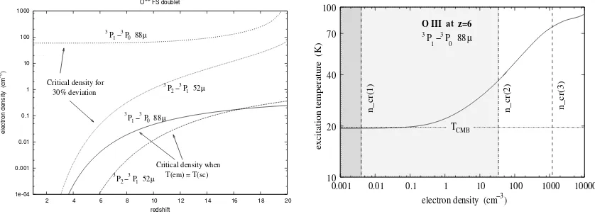
4.8 Three types of critical densities for the O++ _{ion . . . .} ₄₃

5.1 Temperature anisotropy generated from resonant scattering . . . 53

5.2 Constancy ofδCl-s at small angular scales . . . 54

5.3 Minimum detectable abundance of oxygen from Planck and WMAP . . . 57

5.4 Best angular scale for inferring minimal abundances . . . 59

5.5 Improvement of sensitivity limit by averaging over discrete bands . . . 60

5.6 Effect of different foregrounds on temperature anisotropies . . . 66

5.7 Deterioration of minimum abundance limits due to foregrounds . . . 68

(10)

LIST OF FIGURES

6.2 Optical depths in different fine-structure lines for various histories . . . 72

6.3 Temperature anisotropy from OIII line in two different histories . . . 73

6.4 δCl-s generated by scattering in CII line at different redshifts . . . 74

6.5 Temperature anisotropies resulting from all fine-structure lines . . . 75

6.6 δCl-s at large and small angles for different histories . . . 76

6.7 δCl-s atl= 810, or at ten arc-minute scales . . . 77

6.8 Late reionization and corresponding temperature anisotropies . . . 78

6.9 δCl-s at small angular scales for late reionization . . . 79

7.1 Brightness temperature and number density of star-forming halos . . . 90

7.2 Contribution of line emission without correlation with the CMB . . . 92

7.3 Effect of correlation on the emission power spectrum . . . 95

A.1 Linear dependence on optical depth for the observedδCl-s . . . 103

A.2 Different components of the observedδCl-s . . . 104

B.1 Relative change in population for CO rotational levels . . . 109

(11)

List of Tables

2.1 Far-IR and sub-millimeter instrument sensitivities . . . 19

3.1 Change in brightness temperature in Local Group galaxies . . . 24

3.2 Change in brightness temperature for Virgo cluster galaxies . . . 27

5.1 Minimum detectable abundance of oxygen from CMB experiments . . . 56

(12)

Chapter 1

Introduction

The analysis of the Cosmic Microwave Background (CMB) provides a crucial test bed for cosmo-logical models and theories of interaction of matter and radiation during the course of evolution of the universe. The CMB photons received today were released at the redshiftz '1100, when the universe was only 300,000 years old, therefore studying the changes in the thermal spectrum as well as angular intensity distribution of the CMB can yield information about many subsequent events in the cosmic history, like growth of structure formation, reionization of the universe by the first stars, or evolution of the chemical abundances leading to present day values. High precision CMB observations are already giving us unique information about the angular distribution of the temperature fluctuations, as well as their spectral dependence in a wide frequency range. After an year of operation, the WMAP satellite has obtained the first peaks of the CMB power spectrum with an accuracy of a few percent (Hinshaw et al. 2003), and is on its way to provide measure-ments of the temperature anisotropies in the whole sky with an average sensitivity of 35 µK per 0.3◦_×₀_.₃◦_{at the end of the mission (Bennett et al. 2002, Page et al. 2002). HFI and LFI detectors}

of PLANCK spacecraft will provide unprecedented sensitivity in 9 broad band (∆ν/ν∼20−30%) channels, uniformly distributed in the spectral region of the CMB where contribution of different foregrounds are expected to be at a minimum. The ground-based and balloon-borne experiments like Boomerang, APEX, SPT & ACT, will provide complimentary information about the temper-ature fluctuations at small scales (θ.1◦_{), and will also provide very high precision measurements}

of the changes in the background intensity of the CMB inside particular objects in the sky. In this work we have tried to find some additional use for the sensitivities of these forthcoming CMB experiments, by means of the process of resonant scattering of the CMB photons in atomic, ionic or molecular lines. In presence of the peculiar velocity of the scatterer, the change in the brightness temperature of the background CMB photons takes a particularly simple form

∆T(ν) TCMB

= −τν

³v_k c

´

(13)

1. INTRODUCTION

where ∆T(ν) is the change in brightness temperature observed at the line frequency ν, TCMB is the mean temperature of background CMB photons, τν is the optical depth for scattering at

resonance, andvk is the radial component of peculiar motion of the object in the CMB rest frame.

The negative sign arises from the convention of taking velocities positive for motion away from the observer, which results in a decrement of temperature. We found that such decrement is the unique feature of the scattering signal, which might help to distinguish it from the emission in the same line. In fact, the same effect of scattering had been discussed by several authors in the past, but a formal derivation of the effect had been absent. It was first analyzed by Dubrovich (1977, 1993), who followed Sunyaev & Zel’dovich papers (1970, 1980) on influence of electron scattering on CMB angular fluctuations, and coined the term “spatial-spectral fluctuations” to describe the effect of resonant scattering. This effect was analyzed later in detail by Maoli et al. (1994, 1996). These authors were interested in the detection of primordial molecules, like HD, LiH, H2D, HD+ etc., and there were also attempts to observe them experimentally (de Bernardis et al. 1993). We have extended their analysis to the fine-structure transitions of the various atoms and ions of metals like carbon, oxygen, nitrogen etc., which were produced at the end of the dark ages by the first stars. These fine-structure transitions arise from the spin-orbit coupling of the energy levels, and have wavelengths in the far-infrared region which make them suitable for scattering the CMB photons at high redshifts (2.z.30). These lines had been used by Varshalovich, Khersonskii & Sunyaev (1978) as a means to couple matter and radiation at redshifts around 150−300, where the their different adiabatic indices can lead to absorption of CMB in these lines. There are also the hyper-fine transitions arising from spin-spin interaction, but their extremely low cross-sections make these transitions unsuitable for any application with scattering of CMB photons. The other important application we have made is to consider the effect of scattering in the CO rotational lines, which are similar to the molecular lines mentioned above, but have wavelength extending into the sub-millimeter region owing to the larger mass of CO molecule. This feature, together with the fact that CO is the second most abundant molecule in the local universe, makes analysis of scattering in the CO lines very attractive in the low redshift universe (z.2). We shall see that for galaxies in the local universe, the first three rotational lines of CO which are located near the CMB spectrum and therefore have a large number of photons available for scattering, can give us unique information about the motion of these galaxies in the CMB rest frame.

(14)

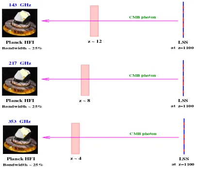
Therefore the higher frequency channels will be sampling the lower redshifts, and provided the fu-ture CMB experiments like ACT measure the CMB sky in many closely packed frequency channels, one would have the possibility to follow the enrichment and ionization history of the universe from such observations. The transverse dimension of the slice will be determined by the beam-width of the experiment, or in case of the integrated signal the angular size of the observing multipole l, corresponding roughly asθ≈π/l. When we shall be speaking of the integrated signal of scattering, our interest will be in all unresolved objects inside this volume, which contribute to the coherent distortion in the angular fluctuation of the CMB. On the other hand, future sub-millimeter interfer-ometers like ALMA shall be able to resolve individual parts of galaxies upto very large distances, and the high sensitivities of these instruments might allow us to detect the signal of scattering from individual gas clouds. The precise frequency dependent nature of the signal will allow us to distinguish it from other emissions which might be coming from the same sources.

We now try to give a rough idea of the effect of scattering on the angular distribution of the temperature fluctuations in the CMB sky. As depicted in Fig.(1.2), the CMB photons arrive to us from the inside of a sphere termed as the last scattering surface (LSS), traveling almost freely except from very occasional effect of scattering (we neglect the scattering by electrons here). The angular distribution of temperature fluctuations inside this sphere is very accurately predicted by cosmological models, which gives us the value of temperature fluctuations in average between two points separated by an angleθ, which we call ∆T(θ), for any value ofθ. Introducing the effect of scattering in this angular distribution, we get

∆T T0

(θ, ν) = e-τν ∆T T0

(θ) ¯ ¯ ¯ ¯

orig.

+ ∆T

T0 (θ, ν)

¯ ¯ ¯ ¯

new

(1.2)

(15)

1. INTRODUCTION

CMB photon

Planck HFI

Bandwidth ~ 25%

LSS

at z=1100

z ~ 12

143 GHz

CMB photon

Planck HFI

Bandwidth ~ 25%

LSS

at z=1100 217 GHz

z ~ 8

CMB photon

z ~ 4 Planck HFI

Bandwidth ~ 25%

LSS

at z=1100 353 GHz

Figure 1.1: Schematic diagram illustrating the advantage of frequency dependent scattering to probe definite redshift intervals. The CMB photons are produced at the epoch of recombination at z ' 1100, which we term as the Last Scattering Surface, and are received by an observing probe like the PLANCK satellite. The signal of resonant scattering is embedded into the observed temperature fluctuations of the CMB, but unlike scattering by electrons, which is equally effec-tive at all redshifts due to the frequency independent Thomson scattering cross-section, resonant scattering by atomic, ionic or molecular lines work only at definite redshift intervals. This redshift interval is defined by the frequency resolution of the experiment, ∆z/z= ∆ν/ν. In fact, for the integrated scattering signal from many unresolved point sources, the effect correspond to a definite volume along the line-of-sight, whose transverse extent depends on the angular scale of observation. For a particular resonant transition, the higher observing frequencies probe the lower redshifts, in accordance with νobs = ν/(1 +z). The illustration above shows the case for scattering by C+

(16)

Observer

L

S

urface cattering ast

CMB photon

Scatterer with peculiar vel.

Observer

CMB photon

L

S

urface cattering ast

Figure 1.2: Schematic diagram illustrating the process of resonant scattering of the CMB photons. One can imagine the primordial temperature fluctuations in the CMB as patterns inside a sphere at redshiftz '1100, which is the Last Scattering Surface. We are at the center of this sphere, and the CMB photons travel almost freely towards us from this surface. However if a photons is scattered by atomic, ionic or molecular lines, it will cause no change in its energy, but will redistribute its direction, as shown in the diagram at left. This will result in a smoothing or blurring of the primordial temperature anisotropies. Moreover, these scatterers will induce their own temperature anisotropy, because of their motion in the CMB rest frame, as shown inright. This motion chiefly corresponds to the large-scale infall velocities of matter into dark matter potential wells, and depends on the redshift of scattering. The observed angular fluctuations are therefore a combination of the smoothed primordial anisotropies and a newly generated motion-induced term.

Having obtained the expression of temperature anisotropies due to scattering, we try to formu-late the corresponding distortion in the power spectrum,Cl-s, which are defined as

∆T T0

(θ, φ) =

∞

X

l=0

l

X

m=−l

almYlm(θ, φ)

Cl =

1 2l+ 1

l

X

m=−l |alm|2

This is the conventional expansion of the temperature fluctuations in spherical harmonics, the second relation defining the sky correlation functionCl-s in terms of the multipole momentsalm.

As a result of resonant scattering, these observedCl-s now are now function of frequency, and we

can write the modification in the CMB power spectrum as

δCl(ν) ≡ Clobs.(ν)−C

prim.

l = τν·C1(ν) +τν2·C2(ν) +O(τν3) (1.3)

δCl(ν) is the expected distortion in the CMB power spectrum at frequency ν, which one obtains

after subtracting the original primordial Cl-s from the observed Cl-s with the scattering signal

(17)

1. INTRODUCTION

with large enough separation, where one observation can be taken to be free of the scattering effect. This is one direct advantage of the frequency dependent nature of resonant scattering, which allows us to pick up extremely small signals by means of comparison at two different frequencies. We see that the resultingδCl-s can be expressed as a power series in the line optical depth, with the

coefficientsC₁₍_ν_),C₂₍_ν_{) etc. as function of frequencies (hence redshifts). Since the optical depths}

in scattering are very small, we are only interested in the first order term, and in fact for small angular scales (l&100) we obtain a particularly simple form for power spectrum distortion

δCl ' −2 τν Clprim. (1.4)

We see that such linear dependence on optical depths provide a massive boost in the amplitude of our effect, since the multipoleCl-s are squares of the temperature fluctuations, so a priory we

should expect theδCl-s to be proportional to τν2. This huge enhancement is the main difference

of our approach from that of Dubrovich and Maoli et al. Such linear dependence arises from a non-zero correlation between the density fluctuations existing between the epoch of recombination and the epoch of scattering (Hern´andez-Monteagudo & Sunyaev 2004), and we see that it can en-hance the scattering signal in the CMB power spectrum by a factor upto a million, if we remember thatτν ∼10−6 for typical cosmic abundances. This forms the basis for our effort to constrain the

enrichment and ionization history of the universe.

The organization of this thesis is as follows. In Ch.2 we present the formulation for the scatter-ing effect, and discuss the nature of the spectrum along random line of sight in comparison with pure absorption spectrum. We also estimate the contribution arising from blurring of primordial anisotropies inside a single scattering cloud. We derive the necessary expressions for brightness temperature and intensities of the scattering signal, and as an application apply them in deter-mining the column densities of CO and molecular gas mass from scattering. Our main example for scattering by individual objects is the detection of peculiar motions of galaxies, which is discussed in Ch.3. In that chapter we try to make use of simultaneous observation of scattering and emission to estimate the optical depths, and also consider the density limits for the effectiveness of scatter-ing. These formalisms are then applied to the Local Group and the Virgo cluster galaxies, where the high velocities of the later make them promising candidates for observing the scattering signal. We demonstrate the method of obtaining the peculiar motions of the galaxies taking into account our own motion in the CMB rest frame. We also tabulate the expected change in the brightness temperatures in the CO lines in these galaxies for some representative column densities.

(18)

at much lower densities. This density limit corresponds to the point upto which we can see an individual object in scattering, and is very low for diffuse electron plasma, and also low for neutral gas containing CO. But when one considers the integrated scattering effect coming from many unresolved point sources in the sky, the coherent distortion in the CMB power spectrum can be caused by objects with densities several times higher, because the contribution of emission from small dense objects is smaller at large angles. This makes it necessary to compute the distortion in the CMB power spectrum as a result of scattering, which we have done in Ch.5.

We have computed the changes in the CMB power spectrum under the limit of very low optical depths, using the CMBFAST code of Seljak & Zaldarriaga (1996) with appropriate modifications. This approach had been used previously by Zaldarriaga & Loeb (2002) to compute the change in the power spectrum arising from scattering in the neutral Li 6708˚Aline. Although this fine-structure transition of Li can give τν greater than unity, it has too short wavelength to be observable by

planned CMB experiments, and is outside the high intensity CMB spectrum even for redshifts 800 < z <1100. The method to overcome the very small optical depth of far-IR fine-structure lines is one of the main focus of this work, which can be achieved by comparing the power spectrum of the same part of the sky from two different frequency channels, which gets rid of the limitation due to the cosmic variance. In Ch.5 we have discussed in detail this approach and the method to set minimum detectable abundances from any given sensitivity of CMB experiments. We also esti-mated the limits when removal of foreground signals in the sky is not complete, thereby worsening the minimum detectable abundances by a factor of 50−200.

(19)

Chapter 2

Resonant Scattering of the CMB

Photons

2.1 Characteristics of the scattering signal

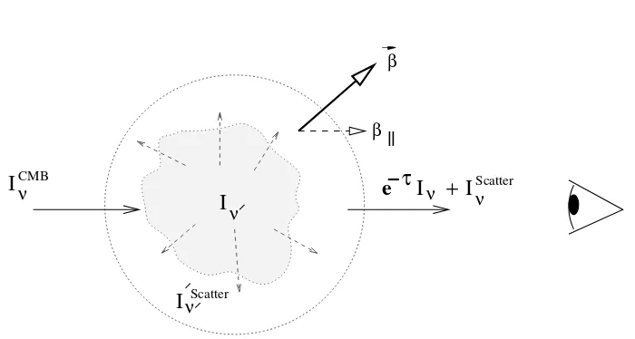
First we discuss the basic underlying effect of resonant scattering and the corresponding change in the background intensity of CMB photons in the direction of the enriched gas. The effect we discuss here had been used by various authors to estimate primarily the distortion in the CMB thermal spectrum due to presence of primordial molecules, but a formal derivation of the effect had been absent. It was first analyzed by Dubrovich (1977, 1993) and later followed-up by various Italian and French groups (Maoli et al. 1994, de Bernardis et al. 1993), who sought to find signals from primordial molecules like HD, LiH etc. in the CMB spectrum. Here we have analyzed the basic underlying principle of this effect and tried to find some other applications. The effect under consideration is equivalent to the well-known kinematic-SZ type distortion (Sunyaev & Zeldovich 1970,1980), as was stated by Dubrovich (1977), but now it is a function of frequency due to the nature of resonant scattering. Scattering of CMB photons in an atomic or molecular line has the combined effect of both loss of CMB photons from the line of sight, and also a gain due to the photons that are scattered into the line of sight. If the scatterer is at rest with respect to the isotropic radiation background, these two effect exactly cancel each other and no change in flux is observed. However, due to the peculiar motion of the enriched gas it will have some non-zero velocity with respect to the CMB rest frame, and as a result will cause a net increase or decrease in the intensity of the background radiation as observed through the gas.

2.1.1 Basic formulation for kSZE type distortion

(20)

2.1 Characteristics of the scattering signal

background (fig.2.1). The incident radiation on the cloud is Iν, which in our case is simply the

Planckian spectrum at frequencyν, andTγ as the mean temperature of background CMB photons

Iν =

2hν3 c2 exp

hhν kTγ −

1i−1 (2.1)

The observed intensity in the direction of the cloud, as mentioned above, consists of two parts:

i)the scattered intensity in the direction of the observer (denoted byIScatter

ν in fig.2.1), andii)the

attenuated intensity of the background CMB radiation: e−τ_I

ν. Assuming non-relativistic velocity

(β¿1), the frequency transformation relating the cloud frame (denoted byprime) and the CMB frame is simply

ν0 =ν(1 +β~·~n) (2.2)

I

β

ν

I

_ν

CMB

Scatter

Scatter ν

I

e

−

τ

I

_ν

+

β

_||

Figure 2.1: Schematic diagram illustrating the change in background intensity through resonant scattering in a moving medium

We can write the intensity in the cloud frame,Iν00, by using the phase-space density conservation

relationI0

ν0 = (ν03/ν3)Iν, which gives

Iν00 = (1−βµ)3A

x3

ex₋₁ (2.3)

Herex≡hν/kTγ is the dimensionless frequency in the observer frame, andA= 2(kTγ)3/(hc)2is a

constant. µis the direction cosine for the angle between direction of motion and the observer, and it shows the intensity in the cloud frame is not isotropic but has a dipole component due to the motion of the cloud. The effect of resonant scattering would be to redistribute this intensity, and the scattered intensity can be written, in the optically thin limit, after integrating over all angles as

I0Scatt

ν0 =τ(ν0)A

x03 ex0

(21)

2. RESONANT SCATTERING OF THE CMB PHOTONS

wherex0_≡_hν0_/kT

0, andτ(ν0) is the line optical depth. The right hand side of eqn(2.4) is solely a function of cloud-frame frequencyν0_{, and hence can be transformed back to observer frame by}

using the same conservation lawIν = (ν3/ν03)Iν00.

For simplicity, let us consider the case of scattering by one single atom or molecule, without any line broadening effect by an ensemble of scatterers. In this idealized case the line profile will simply be aδ-function, and the optical depth will be the product of the line profile with the oscillator strength of the resonant transition (τ ¿1 for the subsequent analysis)

τ(ν0) = πe 2 mec

fi δ(ν0−ν0) (2.5)

This allows us to write the scattered intensity back in observer frame by simply using the properties ofδ-function

IScatt

ν =₍₁ 1

−βµ)3 πe2 mec fi δ(ν

0₋_ν

0)A x

03 ex0

−1 =τ∗₍_ν₎_I

ν

³

1 + _exxex −1 βµ

´

+ O₍_β2₎ _(2.6)

τ∗₍_ν_{) is defined as}_τ∗₍_ν₎_≡₍_πe2_/m

ec)δ(ν−˜ν0), with ˜ν0=ν0(1 +βµ). This shows theshift in the emission profile away from the rest-frame resonant frequency due to the motion of the scatterer. The absorption profile is also shifted by an equal amount, because only photons with frequency ν0₌_ν

0(1−βµ) are in resonance with the moving atom/molecule, and hence lost from the line of sight. The total intensity in the direction of the cloud is then simply the sum of the absorption and scattering terms

Itotal

ν = (1−τν∗)Iν + IνScatt (2.7)

which gives the relative change in intensity in the first order as ∆Iν

Iν

= πe 2 mec

fi δ

¡

ν−ν0(1 +βk)

¢ βk

xex

ex−1 (2.8)

We have usedβk to denote the velocity component in the direction of the observer. This form is

similar to the kinematic-SZ effect, as becomes evident if we rewrite the above equation in terms of temperature distortion upto first order

∆T(ν) Tγ

= τ∗(ν)βk (2.9)

(22)

of motion of the scattering cloud. This can be formally established by writing the emission from the cloud in terms of partial frequency redistribution function

²ν=ni fi

Z ∞

0 dν1

Z +1

−1

dµ1 ϕ(ν0)R(ν,1;ν1, µ1)I0(ν1, µ1) (2.10)

where R(ν, µ;ν1, µ1) is the photon redistribution function, giving the probability that a photon incident on the atom or molecule from direction µ1 and having frequency ν1 will be scattered with frequencyν in the direction of the observer (µ= 1). I0(ν1, µ1) is the incident radiation, and ϕ(ν0) is the line profile for single scattering, which we can again represent with a delta function, ϕ(ν0) =δ(ν1−ν0), assuming zero natural line width. niis the total number of atoms or molecules in

the lower tradition state available for scattering, andfi is the oscillator strength for the transition.

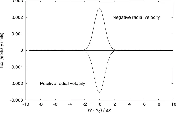
For pure doppler broadening, the frequency redistribution function takes the form of a truncated gaussian (see, e.g. Mihalas 1970), and the resulting emission profile, shown in Fig.(2.2), is a complete gaussian centered at frequencyν0(1 +βk).

-0.003 -0.002 -0.001 0 0.001 0.002 0.003

-10 -8 -6 -4 -2 0 2 4 6 8 10

flux (arbitrary units)

(ν - ν₀) / ∆ν

Negative radial velocity

Positive radial velocity

Figure 2.2: Profile of the emission function of a molecular cloud created by scattering of background CMB photons, taking into account the doppler broadening caused by the thermal motions of atoms or molecules. Positive radial velocity corresponds to motion away from the observer, and negative velocity for motion towards the observer. We get a positive intensity for scattering by cloud moving towards us, and vice versa. Broadening due to any kind of turbulent motion in the gas cloud is neglected, but can easily be taken into account.

2.1.2 Spectrum expected from CMB scattering

(23)

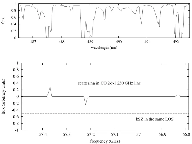
CMB power spectrum, by post-reionization atoms and ions in the redshift range 5−30. The detailed spectrum of distortion caused by scattering on the moving atom, ion or molecule was not of interest, because we were discussing observation with broad-band detectors, whereas in the present chapter we are interested in discrete objects. In that work we solely focussed on the temperature fluctuations averaged over angles exceeding the dimensions of individual objects and halos, because we sought to set constraints on the mean metallicity abundances in the diffuse low density gas, particularly the IGM. In this subsection, we qualitatively discuss the nature of the spectrum resulting from scattering of CMB photons in resonant lines in a molecular cloud. We particularly compare the nature of the predicted signal with the Ly-αabsorption lines in the spectrum of a quasar, and emphasize the distinctive features that might allow to separate out this much weaker signal. We also show the spectrum expected from a particular object, say a galaxy, both when we are able to resolve the object and otherwise.

1 0.8 0.6 0.4 0.2 0

487 488 489 490 491 492

flux

wavelength (nm)

1 0.8 0.6 0.4 0.2 0 -0.2 -0.4 -0.6 -0.8 -1

56.8 56.9

57 57.1

57.2 57.3

57.4

flux (arbitrary units)

frequency (GHz)

scattering in CO 2->1 230 GHz line

kSZ in the same LOS

Figure 2.3: Spectrum of Ly-αforest towards a point source (quasar), and spectrum of scattering of CMB by the same set of gas clouds along the line-of-sight without any quasar in the background. The gas clouds are located atz∼3.

(24)

We note that there is only absorption features present, or reduction of background flux, since quasars being point sources, there can only be loss of photons from the line of sight. In the bottom panel, we show a schematic view of scattering features in the same set of molecular gas along the line-of-sight. The main distinguishing feature is that there is both increment and decrement of background flux (CMB blackbody), depending upon the direction of motion of the cloud. We assumed only the most damped Ly-α systems are dense enough to have neutral molecular gas shielded from the ionizing background. Also shown for comparison is the kinematic SZ signal coming from inter-galactic electrons, which is flat in frequency spectrum.

2.1.3 Temperature distortion from primordial anisotropies

In the preceding discussion we have assumed for simplicity that the intensity of background radiation is isotropic, and neglected the presence of primordial anisotropies. These primordial anisotropies have amplitudes of the order of 10−4₋₁₀−5 _{in the microwave sky, and will be} sup-pressed by the same resonant scattering we have been discussing when one looks through the gas cloud. Since one of our main objectives is to discuss the amplitude of scattering signal from nearby galaxies, whose angular dimension can extend from several arc minutes to one degree scale, we must also consider this additional temperature fluctuation present on those scales. For objects of smaller angular size (few arc seconds) one can neglect the contribution from primordial anisotropies.

We here present only an order of magnitude estimate for this secondary effect. For formulation of the problem we follow Zel’dovich & Sunyaev (1980), where the same effect was discussed for Thomson scattering by cold electrons in clusters, without any peculiar motion of the scattering cloud. The starting point is to note that the primordial intensity field contains angular fluctuations at all angular scales

I(µ0) =I0 "

1 +aµ0+b µ

µ02−1₃

¶ +

∞

X

n=3

CnPn(µ0)

#

(2.11)

where Pn are the Legendre polynomials, andµ0 = cosθ and the angleθ is measured from some

suitable axis. This observed intensity at the directionµ0 _{will be suppressed by the same scattering}

optical depthτν as discussed previously, if a gas cloud happens to be in the same direction. Now,

the resonant scattering couples only with the monopole and quadrupole of the intensity in the same way as electron scattering, and hence the scattered intensity in the direction of the gas cloud will be

I1(µ0) =I(µ0) (1−τν) +I0τν

· 1 +E1b

µ µ02−1₃

¶¸

(2.12) Here the first term is simply the suppression of primordial fluctuations in the direction of the cloud, stating that the fractionτνof photons are lost from the line of sight due to scattering. The second

(25)

the particular resonant transition involved, and have amplitude of the order 0.1 for pure Rayleigh indicatrix.

Therefore The fluctuation in the background intensity inside the object will be ∆I/I0 = (I1(µ0)−I(µ0))/I0, and using the same factor (ex−1)/xex we can write the corresponding tem-perature fluctuation as

∆T(ν) T0

=−τν

ex₋₁

xex [aµ

0 _{+ (1}

−E1)b (µ0 2

−1₃) +

∞

X

n=3

CnPn(µ0)]

=−τν

" ¯ aµ0_{+ ¯}_b

µ µ02

−1 3

¶ +

∞

X

n=3 ¯

CnPn(µ0)

#

(2.13)

Comparing this expression with the formula for motion induced dipole anisotropy, ∆T(ν)/T0= τνβk, we see that for any object of given size, the magnitude of this secondary effect compares

roughly as the ratio of primordial temperature fluctuation at that scale toβk. We also note that

one can not separate out the contribution of primordial dipole from the motion induced dipole at line frequency, since the component of primordial dipole in the direction of motion (angle between the directions corresponding toµ and µ0_{, where} _µ _{marks the direction on motion of the object)}

will always be present in the observed signal. However if one takes the magnitude of primordial dipole to be low (∼10−5_{or less), the observed dipole will be a good tracer of the peculiar motion} of the scatterer.

We can confirm that the temperature fluctuation generated by motion is dominant over this suppression of primosdial anisotropies at all angular scales by some simple order of magnitude estimate. To estimateβk, we assume the linear regime of structure formation, which givesv(z)/c≈

v(0)/c(1 +z)−12. (This relation is true only for matter dominated universe, but we can ignore the corrections due to a particular cosmological model for the present estimates atz >1.) v(0) is the present-day value of large-scale peculiar velocity, which one can take roughly as 600 km s−1_{, but we} remember that this velocity distribution is Gaussian and we have the probability of higher velocities in individual objects. Since the scattering effect will be proportional to the radial component of this motion towards us, we can writevk(z) =v(z)/

√

3, yieldingvk(z)/c= 1.15×10−3 (1 +z)−

1 2. Hence for objects one can resolve, i.e. for galaxies in the local universe, we haveβk ≈10−3. The

intrinsic dipole can not be separated, so we compare the amplitude of scattered intrinsic quadrupole with this value. The effect will be maximized for µ0 _{= 1, and standard ΛCDM model we have}

l(l+ 1)Cl/2π= 1000µK2 at l = 2. Hence the contribution of scattered quadrupole is more than

80 times smaller for the above value of βk. However, the temperature power spectrum has its

maximum around 1◦ _{scale, but even there the maximum probable temperature fluctuation from}

(26)

2.2 Amplitude of the scattering signal

The important point to remember about primordial temperature anisotropies is that they are frequency independent. This means we can separate the small contribution coming from suppression of primordial fluctuations by observing the same patch of sky away from the resonant frequency. CMB anisotropy probes like WMAP has presented us with high angular resolution all sky CMB maps, and hence the contribution from any particular hot or cold spot can be estimated and subtracted from such maps.

2.2 Amplitude of the scattering signal

After discussing the general properties of the scattering signal, we now present the formulation for observable properties of the object like brightness temperature of the object or the beam-averaged flux as might be expected from observation of individual objects. This will help us to set limits on the column density of the scatterer, or mass of the neutral molecular gas, in terms of the characteristics of a fiducial experiment. After presenting the necessary formulation, we inspect which atomic, ionic or molecular lines are most suitable at various redshift ranges. Then we shall proceed to one application: detection of molecular gas from scattering in the nearby universe from scattering. Our main example for application of scattering from individual objects, the detection of peculiar motion of galaxies, is discussed in the next chapter.

The optical depth in scattering is expressed as the product of the number density of the atoms or molecules with the scattering cross-section along the line-of-sight:

τν=

Z

ni σ(ν)dl (2.14)

Here ni is the number density (in cm−3) of the species iunder study, and σ(ν) is the scattering

cross-section at line frequencyν. The cross-section for resonant scattering is expressed in terms of the oscillator strength of the transition invovlved, which have the following form (see, e.g., Rybicki & Lightman 1985 for definitions)

σ(ν) = πe 2 mec

fi(ν)ϕ(ν) (2.15)

fi(ν) = mec

8πe2 gu

gl

µ 1−$_$u

l

gl

gu

¶ c2

ν2 Aul (2.16)

Here fi(ν) is the oscillator strength of the particular transition, which is expressed in terms of

level degeneracy and transition rate. $u and $l are the fraction of atoms/molecules present in

the upper and lower transition levels, andgu and gl are the respective statistical weight. Aul is

(27)

Therefore expressed in terms of the column-density of the scatterer, Ni =Rnidl, the optical

depth due to resonant scattering can be written as τν=$lNi 1

8π µ

gu

gl

¶ µ 1−$_$u

l

gl

gu

¶ c2

ν2Aul ϕ(ν) (2.17) This optical depth creates a distortion in the brightness temperature of the CMB temperature according to the relation ∆T /TCMB(z) = τνβk(z), as shown in the previous section. x is the

shorthand for x ≡ hν/kTCMB(z) = hνobs/kT0, where T0 is the temperature of the background radiation today, and νobs is the observing frequency. The mean intensity received today due to

scattering in the object is readily obtained in comparison with Bν, the mean intensity of the

thermal radiation of the CMB, from the relation (following Zel’dovich & Sunyaev 1969) ∆Jν

Bν

= d lnBν d lnT

µ ∆T T ¶ = xe x

ex₋₁

µ ∆T

T ¶

(2.18) where both Iν and Bν are atνobs. Hence using eqn.(2.1) for the Bνobs, and remembering that νobs=ν/(1 +z), the received intensity gets the following form

∆Jνobs=

xex

(ex₋₁₎2 2hν3

c2 (1 +z)

−3 _τ

ν βk(z) (2.19)

We can simplify the expression in eqn.(2.17) if we write the quantity in the parentheses (1−

$ugl/$lgu) as (1−exp(−x)), because we are interested in the limitTEX ≈TCM B, i.e. when level

populations are completely governed by background CMB temperature, which will be the case for very low density gas in thermal equilibrium with the CMB. Since the usually reported observable quantity is the velocity integrated flux over the telescope beam (Iobs =RIν dv dΩ), we write the

intensity in the same form Iobs= hc

4π

Ωbeam

(1 +z)3 x

(ex₋₁₎ $lNCO

gu

gl

Aul βk(z) (2.20)

In this expression Ωbeamis the telescope beam-width. This observed intensity, integrated ober the

line profile, is the usually reported quantity from experiments. For the small scattering signal, a suitable unit would be mJy·km s−1_{, and we use thhe eqn.(}_3.3_{) to estimate the possibility of} observation from future far-IR or sub-mm experiments.

(28)

1e-04 0.001 0.01 0.1 1

0 2 4 6 8 10 12

beam-averaged flux (mJy km s

-1 )

redshift

CII 158 µ

CI 609 µ

CI 370 µ

C P − P

C

3

3 3

1 0

1 2 3

+

0.01 0.1 1

0.01 0.1 1 10

-1 )

redshift

CO 0-1 2600 µ

CO 1-2 1300 µ

CO 2-3 867 µ

CI 609 µ

CO 2−3

CO 0−1

CO 1−2

C P − P

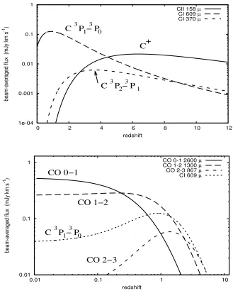
3 ₁3 ₀

Figure 2.4: Expected flux arising from scattering of CMB photons, averaged over a 5000_×₅₀00_beam,

from various species ofcarbon. The column densities for C+_{and neutral C are taken as 10}14_cm−2_, whereas the column density for CO molecule is chosen to be a factor of 10 lower, at 1013 _cm−2_. We neglect any redshift evolution in abundances for this discussion. This figure demonstrates the usefulness of the first two rotational lines of CO, as well as the 492 GHz fine-structure transition of neutral carbon, to probe individual objects at low redshifts. The peculiar velocity of the objects vary asβk(z)≈10−3(1 +z)−

(29)

1e-04 0.001 0.01 0.1 1

0 2 4 6 8 10 12

-1 )

redshift

NII 205 µ

OI 63 µ

OIII 88 µ

N

O

O +

++

Figure 2.5: Same plot as before, showing the flux expected from scattering by other atomic and ionic fine-structure lines. Plotted above are the three most important FS lines of elements other than carbon: the neutral oxygen 63µ, doubly ionized oxygen 88µ, and singly ionized nitrogen 205µ. The column density for all these species is taken at an uniform 1014 _cm−2_{, without any change in} abundance with redshift. The short wavelengths of these lines make them unsuitable for scattering CMB at low redshifts, but for redshiftsz&3 they become important.

2.2.1 Application: column densities of molecular gas

Here we present a simple example for the application of the scattering formulation presented so far. We shall try to estimate the column density of CO moleules,NCO, as can be probed from its lower rotational lines. Our main application for scattering in individual objects, viz. detection of peculiar motion in nearby galaxies, shall be discussed in the next chapter.

We derive the limiting column density of CO molecules that can be probed with future ex-periments like ALMA1_{from the observation of scattering. We assume that the abundance of CO} molecules is low, so that the cloud is optically thin in CO lines (τν <1). We also assume a very

low density gas where line emission from collisional excitation will be more important only for the lowest rotational transition. To begin, from eqn.(3.3) we write the expression for column density of CO molecules

NCO= 4π hc

(1 +z)3 Ωbeam

µ_ex₋₁

x ¶ _g

l/gu

$lAul

ICO vk(z)/c

(2.21)

which we can rewrite, remembering x = kT0/hνobs, in terms of the observing frequency of the

experiment

NCO= 3.6×1015cm−2

µ_{1 +}_z 2

¶3µ _Ω

beam

500_×₅00

¶−1 ₁ $u

µ _A

ul

10−7 _s−1

¶−1_³ _ν

obs

100 GHz ´−1

1

(30)

Experiment / Frequency Wavelength Angular Sensitivity Freq. res.

Instrument (GHz) (µm) Resolution (mJy) (km s−1

) 35 - 100 8500 - 2700 0.500_{- 0.1}00 _0.77 ₂₅

ALMA 100 - 300 2700 - 1300 0.100_{- 0.05}00 _1.2 ₂₅

300 - 400 1300 - 730 0.0500

- 0.0400

2 25

Herschel SPIRE 500 - 1500 200 - 600 2000

- 4000

140 600

Herschel PACS 1600 - 5000 60 - 180 5000 ₃ ₁₇₅

SOFIA 500 - 2000 60 - 700 2000 ₁₀₀ ₂₀

Table 2.1: Spectroscopic sensitivities for current and future IR & sub-mm instruments, in increasing order of frequency. Instruments capable of low resolution spectroscopy are also chosen depending on their frequency coverage. The angular resolution of ALMA is computed assuming an intermediate configuration of 64 antennas, between compacts array and maximum baseline, yielding a resolution of 0.0500_×₍₃₅₀_/ν

obs(GHz)). Spectral sensitivities of ALMA are from Butler & Wootten (1999),

and values for Herschel and SOFIA are taken from respective project websites.

×B

µ _v

k(z)/c

6×10−4 ¶−1µ

ICO mJy km s−1

¶

(2.22)

For example, if we consider the CO 2→1 230.7 GHz line, scattering atz= 1, the observing frequency will be 115.4 GHz. The population at the upper level is $2 = 0.11, and we have Aul= 7.36×10−7s−1. Bis the shorthand for the term in parenthesis in eqn.(2.16), and is roughly

0.8. This corresponds to a column density of 3.0×1015_cm−2_{for an intensity of 1 mJy km s}−1_{. For} the same sensitivity the 3→2 346 GHz line corresponds to a column density of 1.2×1016 _cm−2 because$3= 0.006, and the limits obtained from higher rotational transitions are even worse for very low excitation. However we have assumed the mean value of the large scale motion for these estimates: the limits will go lower for objects with very high peculiar velocity. Also for nearby galaxies (like in the Virgo cluster) scanning with a broader beam (∼0.5 square arc minute) can probe column densities a few times 1013 cm−2 in the CO 230.7 GHz line for similar instrument sensitivity.

(31)

Chapter 3

Scattering & Peculiar Motion of

the Galaxies

3.1 Scattering signal in presence of emission

The effect of resonant scattering in presence of peculiar velocities in far-IR or sub-millimeter lines is extremely attractive, as it might allow us to infer peculiar motions of nearby galaxies in the CMB rest frame. Using higher rotational transitions of CO molecule, or fine-structure lines of neutral carbon, we can also probe the peculiar motion of galaxies at low or intermediate redshifts (z.5). In this separate section we investigate this possibility as an application of scattering observation in individual objects.

As shown in the previous section, the formulation for the change in the background CMB temperature due to resonant scattering in molecular or fine-structure lines is extremely simple, it consists of onlytwoparameters: the optical depth of the scattering cloud at the line frequency,τν,

and the component of its peculiar motion in the CMB rest frame in the direction of the observer, βk (Dubrovich 1977, Maoli et al. 1994),

∆Tb

Tγ

= −τν βk (3.1)

The negative sign comes from the convention of taking βk positive for motion away from the

observer, which gives a decrement in ∆Tb. We take the case of CO molecules as our example, since

we shall be focusing on the scattering in CO rotational lines in nearby galaxies. The change in the brightness temperature observed from scattering, and the velocity integrated intensity, have the form

∆Tbobs(ν) =T0$lNCO c2 8πν2

gu

gl

¡

1−exp(−x)¢

Aulϕ(ν)βk (3.2)

Iobs= hc 4π

1 (1 +z)3

x

(ex₋₁₎ $lNCO

gu

gl

(32)

3.1 Scattering signal in presence of emission

The later have units of mJy km s−1_sr−1_{. We shall be using this expression to estimate the column} density, and hence optical depth, of the scattering species in a fully resolved gas cloud.

3.1.1 Simultaneous observations of scattering and emission

We saw that the amplitude of the scattering signal depends on two parameters: the peculiar mo-tion of the objects towards us, and the optical depth in the line frequency. The optical depth in turns depends upon the column density of the scatterer. Hence if we try to estimate the peculiar motion of galaxies from a decrement of background CMB temperature (which can only be caused by scattering), we must have an accurate idea about the column density of the scatterer. This is where the simultaneous observation of scattering and emission in two different lines become useful. It has never been observed previously because the observation of scattering signal requires very high instrument sensitivity, and also existence of CO molecules in low density regions of galaxies. As we shall see in the next chapter, different rotational levels of CO have different critical densities when scattering becomes observable in that transition. e.g. collisions with hydrogen become more effective for the lowest lying CO rotational level at densities around 2−3 cm−3_{, whereas for the} next transition this density is almost 10 cm−3_{. For galaxies moving with upto 1500 km s}−1_{, both} density limits become 3- or 4-times higher. So it can very well happen that in one line we have emission, and in other we have scattering, from the same molecular cloud. Simultaneous obser-vations at two different frequencies will give usindependent estimate on the density and optical depths.

Let us consider the two lowest transitions of CO rotational system: J=0-1 115 GHz, and J=1-2 230 GHz. Let us consider the local universe, withTEX ≈T0whereT0= 2.726 K. We assume from this low density cloud we have emission due to collision at 115 GHz, but emission is negligible at 230 GHz. If in this neutral cloud the most dominant partner is hydrogen atoms, then the integrated line intensity at 115 GHz for optically thin emission from a homogeneous gas can be written as

I115 GHz= hc

4π NCOnH $0 γ01 (3.4)

We can compute the level population at the lowest level,$0, easily under the assumptionTEX ≈

TCM B, and use this column density with eqn.(3.3) to get the line integrated flux at 230 GHz from

scattering

I230 GHz= µ

x12 exp(x12)−1

¶ g2 g1

$1 ·

I115 GHz nH$0γ01

¸

A21 βk (3.5)

(33)

3. SCATTERING & PECULIAR MOTION OF THE GALAXIES

frame

βk= 1.36×10−2

³ n_H 10cm−3

´ µI_{230 GHz} I115 GHz

¶

(3.6)

where we assumed a 60 K gas cloud in whichγ01= 4.75×10−10 cm3s−1(Balakrishnan et al. 2002), and we haveA21= 7.36×10−7s−1(Chandra et al. 1996).

We still have the uncertainty about the neutral hydrogen density in the gas cloud, for which we can use observation at yet another frequency, like the 21 cm line. We can also use the fine-structure line emission for neutral carbon 492 GHz line, as from Fig.(4.5) we see that collision with neutral hydrogen atoms becomes effective at much lower densities in producing line emission if this FS doublet. So we will have line emission from neutral carbon at 492 GHz similarly as before

I492 GHz= hc

4π NCnH$ CI

0 γ01CI (3.7)

which can be used to get an estimate for nH. Using eqn.(3.6) therefrom we can estimate the peculiar motion of the cloud or galaxy.

We point out that the simple formalism for line emission presented here assumed uniform den-sity gas, without the effect of clumping. In reality for a moderately large beam-width or for an object at larger distance we must emply some filling factor into the computation. For our simple estimate, however, we neglect these complications.

3.1.2 Density limit for the effectiveness of scattering

We briefly point out here the densities which can be probed with scattering, a more detailed discussion on this topic can be found in the next chapter. We concentrate on predominantly neutral gas, where the main collision partner for CO molecules will neutral hydrogen atoms or H2 molecules. The brightness temperature from emission can be written as

Tbem=Tγ

c2 8πν2

(ex₋₁₎2

xex $lNCO nHγlu ϕ(ν) (3.8)

wherenHdensity of the neutral hydrogen atoms (in cm−3), andγluis the collision rate (in cm−3s−1)

from lower to upper level. If we compare this with the brightness temperature arising from scatter-ing in the same line, we arrive at the expression of density at which both scatterscatter-ing and emission contribute equally to the brightness temperature

nH/H₂ = xex (ex₋₁₎2

µ 1−$_$u

l

gl

gu

¶ gu

gl

Aul

γlu βk (3.9)

(34)

3.2 Peculiar motion of nearby galaxies

km s−1_{, such that for local universe the radial component of motion is roughly 350 km s}−1_{, then} this density corresponds to about∼1 hydrogen molecule per cm3_{, or about}_∼_{10 hydrogen atoms} per cm3_{, in neutral gas. In some massve clusters like Virgo, however, the galaxies can attain} unusually high peculiar velocities, of the order of 1500−2000 km s−1. Then this density limits when scattering becomes effective correspondingly becomes higher, as can be seen from Fig.(3.2) for Virgo cluster galaxy M 99.

Since we have for low densities (1−$ugl/$lgu)≈(1−e−x), we can approximately write the

critical density of hydrogen atoms (or molecules) when a gas cloud becomes visible in scattering as

nH/H₂≈ x ex₋₁

Aul

γlu

βk (3.10)

where, as before, xis the shorthand for x≡hν/kTCMB(z) =hνobs/kT0. Now one can see clearly how higher density objects can be probed by scattering if the peculiar motion is high, from the direct dependence of this critical density onβk. We are particularly interested in galaxies having

a positive radial velocity, i.e. galaxies moving away from us with high velocity, since that will give rise todecrementin the background temperature because of scattering. Such negative signal is the unique characteristic of the scattering phenomenon. Strong scattering signal will also be expected from galaxies moving towards us, but since that signal will have the same feature as line emission, it will be impossible to distinguish the scattering case from emission from an increase in background temperature.

3.2 Peculiar motion of nearby galaxies

In this section we discuss the expected change in brightness temperature of galaxies for some low CO column density, which we take fixed at 1013 _cm−2_{. However to minimize the effect of} collision we shall assume that the neutral gas has no more than ∼ 10 hydrogen atoms per cm3 in the scattering cloud. Such extremely low-density objects may provide insufficient shielding for the CO molecules from the ionizing UV background, and detection of the scattering signal might prove to be very difficult. However, we note that such column densities for the CO molecules are at the present observational limit in our Galaxy, deduced from the UV spectra obtained by

Copernicussatellite (Crenny & Federman 2004). It is significantly lower than the column densities obtained from millimeter wavelength studies of emission from molecule-rich gas (e.g. Lambert et al. 1994). Detection of scattering signal from very high velocity galaxies, therefore, may prove to be an important tool for detecting the presence of very low density neutral gas.

(35)

Change in Brightness Temperature for Local Group Galaxies

Name of Vr Position Vcorr VpecCMB ∆Tbfor J=1-0 ∆Tbfor J=2-1

Galaxy (km s−1

) (l, b) (km s−1

) (km s−1

) at 115 GHz at 230 GHz

LMC 275 280.2◦_,₋₃₃_.₃◦ ₊₅₈ ₊₃₃₃ _-30 _-9

SMC 148 302.8◦_,₋₄₄_.₃◦ ₋₃₄ ₊₁₁₄ _-10 _-3

M 31 −315 121.2◦_,₋₂₁_.₆◦ ₋₂₉₀ _-605 ₊₅₅ ₊₁₆

M 32 −205 121.1◦_,₋₂₁_.₉◦ ₋₂₉₁ _-496 ₊₄₅ ₊₁₃

M 33 −181 133.6◦_,₋₃₁_.₅◦ ₋₂₈₇ _-468 ₊₄₃ ₊₁₂

M 110 −241 120.2◦_,₋₂₁_.₄◦ ₋₂₉₁ _-532 ₊₄₈ ₊₁₄

IC 1613 −232 129.7◦_,₋₆₀_.₅◦ ₋₃₃₀ _-562 ₊₅₁ ₊₁₅

IC 342 31 121.0◦_,₋₂₆_.₇◦ ₋₃₂₂ _-301 ₊₂₆ ₊₇

Table 3.1: Expected change in the brightness temperatures from scattering in the CO 115.3 GHz and 230.6 GHz rotational lines. The radial velocity is for the center of the galaxy, ignoring rotation. Considering rotation will result in an increase and decrease from these mean values on the two ends of the spiral arms of an inclined galaxy. The correction velocity, Vcorr, takes into account

the Sun’s motion in the CMB rest frame, and explained in Fig.(3.1). The change in brightness temperature is computed for a CO column density ofNCO= 1013 cm−2and line width 50 km s−1. The brightness temperatures are in units ofµK·km s−1_.

for most galaxies the rotation will result in an increase of temperature distortion at one side of the galaxy and a decrease on the other side. For simplicity we have limited our analysis only to the mean center-of-mass motion of the galaxies, and for more accuracy the radial component of the rotational velocity must be added and subtracted on the two opposite sides. It is also worth to remember that the main component of peculiar motion actually comes from the large-scale motion of the galaxies, as can be seen from the fact that the motion of our Galaxy as a whole in the CMB rest frame is larger than the rotational velocity of the Sun around the center.

3.2.1 Brightness temperature of Local Group galaxies

We now focus attention to our neighboring galaxies, and try to predict the expected increment or decrement in the brightness temperature due to scattering in the CO lines. The obvious reason for studying these nearby objects is that one can resolve small low-density regions inside this galaxies with single-dish telescopes, and of course the absence of any Hubble motion or baricentric velocities in the observed Vr reduces the uncertainty in estimating peculiar motion. However,

most of our local group members, apart from LMC and SMC, are moving towards us, which will give a increment in brightness temperature from scattering. Such increment will be impossible to distinguish from the emission signal coming from the same lines. Also relatively weak peculiar motions of these galaxies forbid studying of most of the density ranges via scattering.

(36)

LMC and SMC move away from us, and might give us a decrement in the CMB temperature. Since temperature decrement is the most definitive sign for scattering signal, we consider galaxies outside our local group, in Virgo cluster, where the high mass of the cluster gives rise to very strong peculiar motions.

3.2.2 Correction due to Sun’s proper motion in the CMB frame

corr

V = V cos θ

V

θ

Sun−CMB

V

Sun − CMB

Sun

GC − CMB

Sun −M31

Sun − CMB

M31

Sun −M31

Sun −M31 Sun − CMB

l=0 b=0

Figure 3.1: Schematic diagram for vector addition, trying to illustrate the approach used for the correction of our own proper motion in the CMB rest frame. The galaxy in the example is chosen to be M 31 (Andromeda), and for the time being we neglect its rotation and focus on its center-of-mass motion. Center of M 31 is situated at the galactic coordinates (l, b) = (121.2◦_,₋₂₁_.₆◦_),

and hasheliocentricradial velocity of 315 km s−1_{towards us. Our own heliocentric motion is 370} km s−1_{in the direction (}_{l, b}_{) = (264}_.₄◦_,₄₈_.₄◦_{), thus making an angle of Θ = 156}◦ _{between the}

vectorsSun-M31andSun-CMB. The correction velocity due to Sun’s proper motion in the CMB rest frame is thereforeVSun-CMB cos(π−Θ), directed in the opposite direction on M 31 for velocity addition.

For estimating the change in brightness temperature at the resonant frequency due to peculiar motion of the galaxies, we must take into consideration our own motion with respect to the CMB. This heliocentric velocity in the CMB rest-frame has been accurately measured from the cosmic dipole by COBE DMR instrument, and we know the Sun is moving with a velocity 369.5 km s−1 towards the direction (l, b) = (264.4◦,48.4◦) in the CMB rest-frame (Kogut et al. 1993). We correct for this motion by adding a correction velocity,Vcorr, to the observed radial motion of the

galaxy

Vcorr=−~n·V~Sun−CM B (3.11)

(37)

with respect to the CMB and the galaxy’s motion towards us (Fig.3.1). This Vcorr can then be

added to the radial motion of the galaxy to get its absolute peculiar motion (more accurately, the component of absolute motion in our direction) in the CMB rest-frame. The result for such velocity estimation and prediction of temperature change due to scattering is listed in Table(3.1) and (3.2).

It is worthwhile to remember that the effect of scattering is sensitive only to the proper motion of the galaxy in the CMB rest frame. Hence for galaxies beyond the local group we must correct for the Hubble expansion either by assuming some definite Hubble constant and distance to the object, or by taking a fixed baricentric velocity of the galaxy cluster and aubtracting it from the observed radial motion. We employ he later technique for analysis of Virgo cluster.

3.2.3 Peculiar motion of galaxies in the Virgo cluster

Next we consider some galaxies from nearby Virgo galaxy cluster, both because of its proximity and because the high mass of Virgo gives rise to unusually high peculiar velocity of some of the galaxies. There are many well-defined spirals in the central region of Virgo whose large angular dimensions may allow us, with future facilities like ALMA, to study small outer sections of the galaxies with very low density. For a distance of almost 20 Mpc, the value of Hubble expansion at Virgo is approximately 1300 km s−1_{, and we must subtract this value from the observed radial motion of} the galaxies in the cluster. We show below that because of the very high peculiar velocities inside the Virgo cluster, temperature decrement as low as−100µK can be observed in galaxies like M88 and M99.

To derive the peculiar motion of the member galaxies in Virgo, we proceed as following. The observed radial motion of the galaxies hasthreecomponents:

Vr=Vh+V~pec·ˆn+V~gal·ˆn (3.12)

whereVh is the Hubble expansion velocity at the center of the Virgo cluster,Vpec is the peculiar

motion of the cluster as a whole in the CMB rest frame (motion in the Great Attractor potential), and Vgal is the Virgocentric peculiar motion of the galaxy itself. ˆn is the unit vector in our

direction to pick the appropriate radial component. The effect of scattering under discussion does not depend on the Hubble expansion velocity, as the scattering of CMB photons by atoms and molecules depends only on their velocity in the CMB rest frame. We can subtract theVh term by

assuming some definite Hubble constant (e.g. H0 = 71 km s−1Mpc−1from WMAP data, Spergel et al. 2003) and multiplying it by the distance of Virgo cluster (∼18 Mpc, from observations of Cepheids, Freedman et al. 1994). Alternatively, we can subtract a fixedcluster velocityfrom the observed radial motion of the galaxy, and take the remainder as the galaxy’s peculiar motion in the CMB rest frame. This cluster velocity already has the Hubble expansion term inside it

(38)

Peculiar Motion and Change in Brighness Temperature for Virgo Cluster Galaxies in CO Lines

Name of Vr Vpec Position Vcorr ∆Tb for J=2-1

Galaxy (km s−1

) (km s−1

) (l, b) (km s−1

) (µK·km s−1)

NGC 4406 (M 86) -227 -1487 279.1◦

,77.6◦ _+263.1 _+32.8

NGC 4569 (M 90) -235 -1495 288.5◦

,75.6◦ _+330.5 _+31.2

NGC 4419 -261 -1521 276.5◦

,76.6◦ _+330.4 _+31.9

IC 3453 +2559 +1299 281.4◦

,76.9◦

+328.9 -43.6

NGC 4388 +2524 +1264 279.1◦

,74.3◦ _+336.2 _-42.9

NGC 4254 (M 99) +2407 +1147 270.4◦

,75.2◦

+334.6 -39.7

NGC 4607 +2257 +997 293.5◦

,74.6◦ _+331.0 _-35.6

Table 3.2: Galaxies in the Virgo cluster, and the predicted change in brightness temperature from scattering in the CO 230 GHz line. We take CO column density to be equal to 1013 _cm−2_{, and} broadening of the line as 50 km s−1_{. High-velocity galaxies in the direction both towards us} and away from us are chosen to demonstrate the effect of increment or decrement of brightness temperature due to scattering. Vr is the observed radial motion (heliocentric velocity) of the

galaxy. The correction velocity Vcorr is explained through Fig.(3.1). For estimating the peculiar

velocity (radial component), we have subtracted from the observed radial motion the baricentric velocity of the Virgo cluster, which we assumed to be 1200 km s−1_.

This value of baricentric velocity of Virgo cluster comes from observations of Federspiel, Tam-mann & Sandage (1998), and we use this fixed value to obtain the peculiar motion of the galaxy: VCMB

g = Vr−Vcl. This of course leaves the room for uncertainty from the peculiar motion of

the cluster itself in the CMB frame, and the actual result can increase or decrease due to this uncertainty. Finally, we correct for our own peculiar motion in the CMB rest frame by the method described previously, and the result for such computations and corresponding increment or decre-ment in brightness temperatures are tabulated in Table(3.2).

In the table we have only shown the scattering brightness for the second rotational line, as this transition allows us to probe higher densities in scattering. The main distinguishing feature is the

signof change in brightness temperature, which is clearly demonstrated. If we assume some low density gas, with molecular hydrogen density ∼10 cm−3_{, then we shall have emission from the} J = 0−1 115 GHz line, and simultaneous measurement of scattering and emission will allow us to obtain independent measure of the column density of CO molecules. For an assumed column density of 1013_cm−2_{and molecular density of}_∼_{10 cm}−3_{, the brightness temperature in emission} in the first rotational line is 35µK, which is of course always positive in sign.

Basu, Kaustuv (2004): CMB observations and the metal enrichment history of the universe. Dissertation, LMU München: Fakultät für Physik

CMB Observations and the

Metal Enrichment History

of the Universe

Kaustuv moni Basu

Max-Planck-Institut f¨

ur Astrophysik

Garching

Dissertation der Fakult¨

at f¨

ur Physik

der

Ludwig-Maximilians-Universit¨

at

M¨

unchen

Acknowledgements

Abstract

Contents

List of Figures

List of Tables

Chapter 1

Introduction

L

S

S

L

S

S

Chapter 2

Resonant Scattering of the CMB

Photons

2.1

Characteristics of the scattering signal

2.1.1

Basic formulation for kSZE type distortion

I

I

I

I

e

−

τ

I

+

||

2.1.2

Spectrum expected from CMB scattering

2.1.3

Temperature distortion from primordial anisotropies

2.2

Amplitude of the scattering signal

C P − P

C P − P

C

+

CO 2−3

CO 0−1

CO 1−2

C P − P

2.2.1

Application: column densities of molecular gas

Chapter 3

Scattering & Peculiar Motion of

the Galaxies

3.1

Scattering signal in presence of emission

3.1.1

Simultaneous observations of scattering and emission

3.1.2

Density limit for the effectiveness of scattering

3.2

Peculiar motion of nearby galaxies

3.2.1

Brightness temperature of Local Group galaxies

3.2.2

Correction due to Sun’s proper motion in the CMB frame

3.2.3

Peculiar motion of galaxies in the Virgo cluster

_||