1
Complexity of some of Pyramid Graphs Created from a Gear Graph
Jia-Bao Liu
1and S. N. Daoud
2,31 School of Mathematics and Physics, Anhui Jianzhu University, Hefei 230601, P.R. China.
2Department of Mathematics and Computer Science, Faculty of Science, Menoufia University, Shebin El Kom 32511, Egypt.
3Department of Mathematics, Faculty of Science, Taibah University, Al-Madinah 41411, Saudi Arabia.
[email protected],[email protected]
Abstract
In mathematics, one always aims to obtain new frameworks from specific ones. This also stratified to the regality of graphs, where one can produce numerous new graphs from a specific set of graphs. In this work we define some classes of pyramid graphs created by a gear graph and we derive straightforward formulas of the complexity of these graphs, using linear algebra matrix analysis techniques and employing knowledges of Chebyshev polynomials.
Keywords:
Complexity; Chebyshev Polynomials; Gear graph; Pyramid graphs.Mathematics Subject Classification:
05C05, 05C50.
1.
Introduction
The graph theory is a theory gathering computer science and mathematics, permitting to solve considerable problems in several fields ( telecom, social network, molecules, computer network, genetics,…) by designing them by graphs and facilitate them by idealistic cases such as the spanning trees See [ 1-10 ].
A spanning tree of a finite connected graph G is a maximal subset of the edges that contains no cycle, equivalently a minimal subset of the edges that connects all the vertices. The history of enumerating number of spanning trees
(G)
of a graph G dates back into year 1842 in which the physicist of Kirchhoff [11] gave the matrix tree theorem established on the determinants of a certain matrix gained from the Laplacian matrix Ldefined by the difference between the degree matrix D and adjacency matrix A of a graph G. That is
if
1 if and is adjacent to ,
0 otherwise i
i j
a i j
L i j i j
=
= −
where ai denotes the degree of vertex .i
This method allows beneficial results for a graph comprising a small number of vertices, but it will be infeasible for large graph. There are one more methods for calculating ( )G . Let 12...k =0 denote the eignvalues of the matrix Lof a graph G with n vertices. Kelmans and Chelnokov [12] have derived that
1
1
1
( ) .
k k i
G k
−
=
=
Many works have conceived techniques to derive the number of spanning tree of a graph. Now, we give the following Lemma:
Lemma 1.1[13]
2
1
( ) det ( c c)
G k I D A
k
= − + where Ac and Dc are the adjacency and degree matrices of c
G , the complement of G
, respectively, and I is the kk identity matrix.
The characteristic of this formula is to express ( G)straightway as a determinant rather than in terms of cofactors as in Kirchhoff theorem or eigenvalues as in Kelmans and Chelnokov formula.
2.
Chebyshev Polynomial
In this part we insert some relations regarding Chebyshev polynomials of the first and second types which we use it in our calculations.
2
We start from their definitions, see Yuanping, et. al. [14]. Let A xn( ) be n n matrix such that
2 1 0 0
1 2 1
( ) 0 0 .
1
0 1 2
0 n
x x A x
x
−
− −
=
−
−
Furthermore, we rendering that the Chebyshev polynomials of the first type are defined by
1
( ) cos( cos ) n
T x = n − x (1)
The Chebyshev polynomials of the second type are defined by
1
1 1
1 sin ( cos )
( ) ( )
sin (cos )
n n
d n x
U x T x
n dx x
−
− = = − (2)
It is easily confirmed that
1 2
( ) 2 ( ) ( ) 0
n n n
U x − xU − x +U − x = (3) It can then be shown from this recursion that by expanding detA xn( ) one obtains
( ) det( ( )), 1
n n
U x = A x n (4) Moreover by solving the recursion (3), one gets the straightforward formula
2 1 2 1
2
( 1) ( 1)
( ) , 1,
2 1
n n
n
x x x x
U x n
x
+ +
+ − − − −
=
−
(5)
where the conformity is valid for all complex
x
(except atx
=
1
, where the function can be taken as the limit). The definition of Un( )x easily yields its zeros and it can therefore be confirmed that1 1 1
1
( ) 2 ( cos )
n n n
j
j
U x x
n
− − −
=
=
− (6)One further notes that
1
1( ) ( 1) 1( )
n
n n
U − −x = − −U − x (7)
From Eqs. (6) and (7) , we have:
1
2 1 2 2
1
1
( ) 4 ( cos )
n n n
j
j
U x x
n
− − −
=
=
− (8)Finally, straightforward manipulation of the above formula gets the following formula (9), which is highly beneficial to us latter:
1 2
1
1
2 2
( ) ( 2 cos )
4 n n
j
x j
U x
n
− −
=
+
=
− (9)Moreover, one can see that
2
2 2
1 2 2
1 1 (2 1)
( )
2(1 ) 2(1 )
n n
n
T T x
U x
x x
−
− − −
= =
− − , (10)
2
2 2
1 1 1
( ) [( 1 1) ( 1 ) ] 2
n n
n
T x x
x x
= − + + − . (11)
Now we introduce the following important two Lemmas.
Lemma 2.1 [15]Let B xn( ) be nn Circulant matrix such that
0 1 1 0
0 1
1
( ) .
1
1 0
0 1 1 0
n
x
B x
x
=
Then for n3,x 4, one has
2( 3) 1
det( ( )) [ ( ) 1].
3 2
n n
x n x
B x T
x
+ − −
= −
3
Lemma 2.2 [16]
If AFn n , BFn m , CFm n and DFm m . Suppose that Aand D are nonsingular matrices, then:
1 1
det A B det(A BD C) detD detA det(D CA B).
C D
− −
= − = −
This Lemma give a type of symmetry for some matrices which simplify our calculations of the complexity of graphs studied in this paper.
3.
Main Results
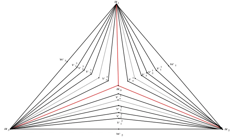
Definition 3.1 The pyramid graph (m)
n
A is the graph created from the gear graph Gm+1 with vertices
0 1 2 1 2
{u ;u u, ,...,um;w w, ,...,wm} and m sets of vertices, say, 1 1 1 2 2 2
1 2 1 2 1 2
{ , ,..., }, { , ,..., },...,{ m, m,..., m},
n n n
v v v v v v v v v
such that for all i =1, 2,...,n the vertex
v
ij is adjacent to uj and uj+1,where j=1, 2,...,m−1, andm i
v is adjacent to
1
u and um. See Fig. (1) .
Fig. 1 The pyramid graph (3)
n A
Theorem 1 For n0,m3, ( (m)) 2mn[( 2 2 3 )m ( 2 2 3 )m 2( 1) ].m n
A n n n n n
= + + + + + − + − +
Proof. Using Lemma 1.1, we have
( )
2 2
1 1
( ) det(( 2 1) )
( 2 1) ( 2 1)
m c c
n
A mn m I D A
mn m mn m
= + + − + =
+ + + +
1
u
2
u
3
u
1
w
2
w
3
w
0
u
1 n
v
1 1
v
1 2
v
1 3
v
2 1
v
2 2
v
2 3
v
2 n
v
3 1
v 3 2
v 3
3
v
3 n
4
( 1) 0 0 0 1 1 1 1
0 2( 2) 1 1 0 1 1 0 0 0 1 1 1 1 1 1 0 0
1 0 1 0 0 0 0 1 1 1 1 1 1
1 1 1 0 0 0 0 1 1 1 1
1 1 1 1 0 0 0 0 1 1
1 1
0 1 1 2(
det
m n +
+
2) 1 1 0 0 1 1 1 1 1 1 0 0 0 0
1 0 0 1 1 3 1 1 1 1 1 1 1 1 1 1
1 1 1 1 1 1 1 1 1 1
1 1
1 0 1 1 1 1 1 1 1 1
1 0 1 1 0 1 1 3 1 1 1 1
n+
1 1 1 1
1 0 0 1 1 0 1 1 1 1 3 1 1
1
0 0 1 1 1 1 1 1
1 0 0 1 1 1 1 1
1 0 0 1 1 1 1 1
1 1 0
1 1 0 1
1 1
1 1 1 0
1 1 0 1 1 1 1
0 1 1 0 1 1 1 1
1
1 0 1 1 0 1 1 1 1 1 1 3
Let j =(1 1) be the 1n matrix with all one, and Jn be the n n matrix with all one. Set a=2n+4 and
2 1
b=mn+ m+ . Then we obtain:
( ) 2
1 0 0 1 1
0 1 1 0 1 1 0 0 0
1 0 0 1 0
1 0
1 0 0 1
0 1 1 1 1 0 0 0 0
1 0 0 1 1 3 1 1
1 0 1 1
1
( m ) det
n
m j j
a j j
j j
j
a j j
j j
A b
+
=
1
1 0 1
1 0 1 1 0 1 1 3
0 0
0
2
0
0 0
t t t t t
t
m n m n
t
t
t t t t t
j j
j j j j j
j
I J
j j
j j j j j
+
5
20 0 1 1
1 1 0 1 1 0 0 0
1 0 0 1 0
1 0
1 0 0 1
1 1 1 1 0 0 0 0
0 0 1 1 3 1 1
1 0 1 1
1 det
b j j
b a j j
j j
j
b a j j
b j j
b
=
1
1 0 1
0 1 1 0 1 1 3
0 0
0
2
0
0 0
t t t t t
t
m n m n
t
t
t t t t t
b j j
bj j j j j
j
I J j
j
bj j j j j
+
1 0 0 1 1
1 1 1 0 1 1 0 0 0
1 0 0 1 0
1 0
1 0 0 1
1 1 1 1 1 0 0 0 0
1 0 0 1 1 3 1 1
1 0 1 1
1 det
j j
a j j
j j
j
a j j
j j
b
=
1
1 0 1
1 0 1 1 0 1 1 3
1 0 0
0
2
0
1 0 0
t t t t t
t
m n m n
t
t
t t t t t
j j
j j j j j
j
I J j
j
j j j j j
+
1 0 0 1 1
0 1 1 1 0 0 1 0 0
1 1 1 0 0
0 0
1 1 0 0
0 1 1 0 0 1 1 0 0
0 0 0 1 1 2 0 0 0 0
1 0 1 0
1 det
j j
a j j
j
a j j
b
− − − −
− − −
−
− − − −
=
1
1 0 0
0 0 1 1 0 0 0 2 0 0
0 0 0 0 0
0
2
0
0 0 0 0 0
t t
t
m n t
t
t t
j j j
I j
j
j j
6
1 1 1 0 0 1 0 0
1 1 1 0 0
0 0
1 1 0 0
1 1 0 0 1 1 0 0
0 0 1 1 2 0 0 0 0
1 0 1 0
1 det
1 1
a j j
j
a j j
b
− − − −
− − −
−
− − − −
=
0 0
0 1 1 0 0 0 2 0 0
0 0 0 0
0
2
0
0 0 0 0
t t
t
m n t
t
t t
j j
j
I j
j
j j
Using Lemma 2.2, yields
( ) 1 1 1
( ) det det( ) 2
2 2
m mn
n
mn mn
A B
A A B C
C I
b b I
= = −
2
2 2 2( 1) 2( 1) 2 2 0 0 2
2 2 2 2( 1) 2( 1) 2 0
2( 1) 2 0
2( 1)
2( 1) 2 0
2 2( 1) 2( 1) 2 2 0 0 2 2
1
2 2 det
0 0 2 2 4 0 0
2 0
2
mn m
a n n n n
n a n n n
n n
n
n n
n n n n a
b
−
+ + + + − −
+ + + + −
+ +
+
+ +
+ + + + − −
=
2 0 0
0 2 2 0 0 0 4
Using Lemma 2.2 again, yields
2
( ) 2 2 1
( ) det det( )
4 4
m n m m n
m n
m m
D E
A D E F
F I
b b I
= − = −
( )
2 ( 3) 2( 2) 2( 2) ( 3)
( 3) 2 ( 3) 2( 2)
2( 2) 2
( ) det
2( 2)
2( 2) ( 3)
( 3) 2( 2) 2( 2) ( 3) 2
mn m
n
a n n n n
n a n n
n A
n b
n n
n n n n a
+ + + +
+ + +
+
=
+
+ +
+ + + +
7
( )
(2 3) 0 ( 1) ( 1) 0
0 (2 3) 0 ( 1)
( 1)
2 2
( ) det
( 1) 2
( 1) 0
0 ( 1) ( 1) 0 (2 3)
mn m n
a n n n
a n n
n b
A
n
b m n m
n
n n a n
− − + +
− − +
+
=
+
+ +
+
+ + − −
1
(2 3)
0 1 1 0
( 1)
(2 3)
0 0 1
( 1) 2 ( 1)
1 det
2
1
1 0
(2 3)
0 1 1 0
( 1)
m n m
a n
n
a n
n n
m n m
a n
n
+
− −
+
− −
+
+
=
+ +
− −
+
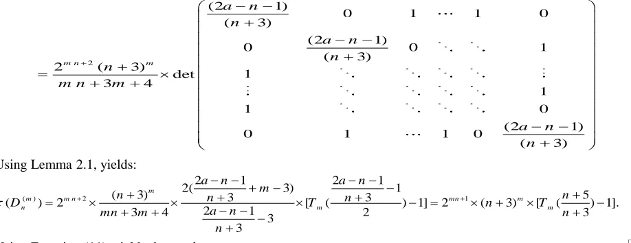
Using Lemma 2.1, yields
( ) 1
2 3 2 3
2( 3) 1
( 1) 1 1
( ) 2 [ ( ) 1]
2 3
2 3 2
1 m
m m n
n m
a n a n
m
n n n
A T
a n
mn m
n
+
− − + − − − −
+ + +
= −
− −
+ + −
+
1
2
2 ( 1) [ ( ) 1].
1
mn m
m
n
n T
n
+ +
= + −
+
Using Equation (11), yields the result.
Definition 3.2 The pyramid graph (m)
n
B is the graph created from the gear graph Gm+1 with vertices
0 1 2 1 2
{u ;u u, ,...,um;w ,w ,...,wm} with double internal edges and m sets of vertices, say,
1 1 1 2 2 2
1 2 1 2 1 2
{ , ,..., }, { , ,..., },...,{ m, m,..., m}
n n n
v v v v v v v v v , such that for all i =1, 2,...,n the vertex j i v is
adjacent to uj and uj+1, where j =1, 2,...,m−1, and
m i
v is adjacent to u1 and um.See Fig. 2 .
Fig. 2 The pyramid graph (3)
n B
1
w
2
w
3
w
0
u
1 n
v
1 1
v
1 2
v
1 3
v
2 1
v
2 2
v
2 3
v
2 n
v
3 1
v 3 2
v 3 3
v
3 n
v
1
u
2
u
3
8
Theorem 2 For n0,m3, ( )
(Bnm ) 2mn[(n 3 2 n 2 )m (n 3 2 n 2 )m 2(n 1) ].m
= + + + + + − + − +
Proof. Using Lemma 1.1, we get:
( )
2 2
1 1
( ) det(( 2 1) )
( 2 1) ( 2 1)
m c c
n
B mn m I D A
mn m mn m
= + + − + =
+ + + +
(2 1) 1 1 1 1 1 1 1
1 (2 5) 1 1 0 1 1 0 0 0 1 1 1 1 1 1 0 0
1 0 1 0 0 0 0 1 1 1 1 1 1
1 1 1 0 0 0 0 1 1 1 1
1 1 1 1 0 0 0 0 1 1
1 1
1 1
det
m n
+ − − −
− +
− 1 (2 5) 1 1 0 0 1 1 1 1 1 1 0 0 0 0
1 0 0 1 1 3 1 1 1 1 1 1 1 1 1 1
1 1 1 1 1 1 1 1 1 1
1
1
1 0 1 1 1 1 1 1 1 1
1 0 1 1 0 1 1 3 1 1 1
n+
1 1 1 1 1
1 0 0 1 1 0 1 1 1 1 3 1 1
1
0 0 1 1 1 1 1 1
1 0 0 1 1 1 1 1
1 0 0 1 1 1 1 1
1 1 0
1 1 0 1
1
1
1 1 1 0
1 1 0 1 1 1 1
0 1 1 0 1 1 1 1
1
1 0 1 1 0 1 1 1 1 1 1 3
Let j=(1 1) be the 1n matrix with all one, and Jnbe the n n matrix with all one. Set a=2n+5 and
2 1
b=mn+ m+ . Then we get:
( ) 2
2 1 1 1 1 1
1 1 1 0 1 1 0 0 0
1 0 0 1 0
1 0
1 0 0 1
1 1 1 1 1 0 0 0 0
1 0 0 1 1 3 1 1
1 0 1 1
1
( m ) det
n
m j j
a j j
j j
j
a j j
j j
B b
+ − −
−
−
=
1
1 0 1
1 0 1 1 0 1 1 3
0 0
0
2
0
0 0
t t t t t
t
m n m n
t
t
t t t t t
j j
j j j j j
j
I J
j j
j j j j j
+
9
21 1 1 1
1 1 0 1 1 0 0 0
1 0 0 1 0
1 0
1 0 0 1
1 1 1 1 0 0 0 0
0 0 1 1 3 1 1
1 0 1 1
1 det
b j j
b a j j
j j
j
b a j j
b j j
b
− −
=
1
1 0 1
0 1 1 0 1 1 3
0 0
0
2
0
0 0
t t t t t
t
m n m n
t
t
t t t t t
b j j
bj j j j j
j
I J j
j
bj j j j j
+
1 1 1 1 1
1 1 1 0 1 1 0 0 0
1 0 0 1 0
1 0
1 0 0 1
1 1 1 1 1 0 0 0 0
1 0 0 1 1 3 1 1
1 0 1 1
1 det
j j
a j j
j j
j
a j j
j j
b
− −
=
1
1 0 1
1 0 1 1 0 1 1 3
1 0 0
0
2
0
1 0 0
t t t t t
t
m n m n
t
t
t t t t t
j j
j j j j j
j
I J j
j
j j j j j
+
1 1 1 1 1
0 ( 1) 2 2 1 0 0 1 0 0
2 1 1 0 0
0 0
2 1 0 0
0 2 2 ( 1) 0 0 1 1 0 0
0 1 1 2 2 2 0 0 0 0
2 1 2 0
1 det
j j
a j j
j
a j j
b
− −
+ − − − −
− − −
−
+ − − − −
=
2
2 1 0
0 1 2 2 1 0 0 2 0 0
0 2 2 0 0
2
2 2
2
0 2 2 0 0
t t t t
t t
m n t
t t
t t t t
j j j j j j
I j
j j
j j j j
10
( 1) 2 2 1 0 0 1 0 0
2 1 1 0 0
0 0
2 1 0 0
2 2 ( 1) 0 0 1 1 0 0
1 1 2 2 2 0 0 0 0
2 1 2 0
1 det
2
a j j
j
a j j
b
+ − − − −
− − −
−
+ − − − −
=
2 1 0
1 2 2 1 0 0 2 0 0
2 2 0 0
2
2 2
2
2 2 0 0
t t t t
t t
m n t
t t
t t t t
j j j j
j j
I j
j j
j j j j
Using Lemma 2.2, yields
( ) 1 1 1
( ) det det( ) 2
2 2
m mn
n
mn mn
A B
B A B C
C I
b b I
= = −
2
(2 2 2) 3 4 4( 1) 4( 1) 3 4 2 0 0 2
3 4 (2 2 2) 3 4 4( 1) 4( 1) 2 0
4( 1) 3 4 0
4( 1)
4( 1) 3 4 0
3 4 4( 1) 4( 1) 3 4 (2 2 2) 0 0 2 2
1
2 2 det
2 2 4 4 4 0 0
4
mn m
a n n n n n
n a n n n n
n n
n
n n
n n n n a n
b
−
+ + + + + + − −
+ + + + + + −
+ +
+
+ +
+ + + + + + − −
=
0
4
4 2 0
2 4 4 2 0 0 4
Using Lemma 2.2 again, yields
2
( ) 2 2 1
( ) det det( )
4 4
m n m m n
m n
m m
D E
B D E F
F I
b b I
= − = −
( )
(2 2 4) (3 7) 4( 2) 4( 2) (3 7)
(3 7) (2 2 4) (3 7) 4( 2)
4( 2) 2
( ) det
4( 2)
4( 2) (3 7)
(3 7) 4( 2) 4( 2) (3 7) (2 2 4)
mn m n
a n n n n n
n a n n n
n B
n b
n n
n n n n a n
+ + + + + +
+ + + + +
+
= +
+ +
+ + + + + +
11
( )
(2 3) 0 ( 1) ( 1) 0
0 (2 3) 0 ( 1)
( 1)
2 4
( ) det
( 1) 4
( 1) 0
0 ( 1) ( 1) 0 (2 3)
mn m n
a n n n
a n n
n b
B
n
b m n m
n
n n a n
− − + +
− − +
+
=
+
+ +
+
+ + − −
2
(2 3)
0 1 1 0
( 1)
(2 3)
0 0 1
( 1)
2 ( 1)
1 det
4
1
1 0
(2 3)
0 1 1 0
( 1)
m n m
a n
n
a n
n n
m n m
a n
n
+
− −
+
− −
+
+
=
+ +
− −
+
Using Lemma 2.1, yields
( ) 2
2 3 2 3
2( 3) 1
( 1) 1 1
( ) 2 [ ( ) 1]
2 3
4 2
3 1 m
m m n
n m
a n a n
m
n n n
B T
a n
mn m
n
+
− − − −
+ − −
+ + +
= −
− −
+ + −
+
1
3
2 ( 1) [ ( ) 1].
1
mn m
m
n
n T
n
+ +
= + −
+
Using Equation (11), yields the result. Definition 3.3 The pyramid graph (m)
n
C is the graph created from the gear graph Gm+1 with vertices
0 1 2 1 2
{u ;u u, ,...,um ;w w, ,...,wm} with double external edges and m sets of vertices, say,
1 1 1 2 2 2
1 2 1 2 1 2
{ , ,..., }, { , ,..., },...,{ m, m,..., m}
n n n
v v v v u v v v v , such that for all i =1, 2,...,n the vertex j i v is
adjacent to uj and uj+1,where j =1, 2,...,m−1,and
m i
v is adjacent to u1 and um.See Fig. 3.
Fig. 3. The pyramid graph (3)
n C
1
w
2
w
3
w
0
u
1
n
v
1 1
v
1 2
v
1 3
v
2 1
v
2 2
v
2 3
v
2
n
v
3 1
v 3 2
v 3 3
v
3
n
v
1
u
2
u
3
12
Theorem 3 For n0,m3, ( )
(Cnm ) 2mn[(n 4 2n 7 )m (n 4 2n 7 )m 2(n 3) ].m
= + + + + + − + − +
Proof: Using Lemma 1.1, we have:
( )
2 2
1 1
( ) det(( 2 1) )
( 2 1) ( 2 1)
m c c
n
C mn m I D A
mn m mn m
= + + − + =
+ + + +
( 1) 0 0 0 1 1 1 1
0 2( 3) 0 1 1 0 0 1 1 0 0 0 1 1 1 1 1 1 0 0
0 1 0 1 0 0 0 0 1 1 1 1 1 1
1 1 1 1 0 0 0 0 1 1 1 1
1 1 1 1 1 0 0 0 0 1 1
1 0 1
0 0 1 1 0 2(
det
m n +
+
3) 1 1 0 0 1 1 1 1 1 1 0 0 0 0
1 0 0 1 1 3 1 1 1 1 1 1 1 1 1 1
1 1 1 1 1 1 1 1 1 1
1 1
1 0 1 1 1 1 1 1 1 1
1 0 1 1 0 1 1 3 1 1 1 1
n+
1 1 1 1
1 0 0 1 1 0 1 1 1 1 3 1 1
1
0 0 1 1 1 1 1 1
1 0 0 1 1 1 1 1
1 0 0 1 1 1 1 1
1 1 0
1 1 0 1
1 1
1 1 1 0
1 1 0 1 1 1 1
0 1 1 0 1 1 1 1
1
1 0 1 1 0 1 1 1 1 1 1 3
Let j=(1 1) be the 1n matrix with all one, and Jn be the n n matrix with all one. Set a=2n+6 and
2 1
b=mn+ m+ . Then we have:
( ) 2
1 0 0 1 1
0 0 1 1 0 0 1 1 0 0 0
0 1 0 0 1 0
1 1 0
1
1 0 0 0 1
0 0 1 1 0 1 1 0 0 0 0
1 0 0 1 1 3 1 1
1 0 1 1
1
( m ) det
n
m j j
a j j
j j
j
a j j
j j
C b
+
=
1
1 0 1
1 0 1 1 0 1 1 3
0 0
0
2
0
0 0
t t t t t
t
m n m n
t
t
t t t t t
j j
j j j j j
j
I J j
j
j j j j j
+
13
20 0 1 1
0 1 1 0 0 1 1 0 0 0
1 1 0 0 1 0
1 0
1
1 0 0 0 1
0 1 1 0 1 1 0 0 0 0
0 0 1 1 3 1 1
1 0 1 1
1 det
b j j
b a j j
j j
j
b a j j
b j j
b
=
1
1 0 1
0 1 1 0 1 1 3
0 0
0
2
0
0 0
t t t t t
t
m n m n
t
t
t t t t t
b j j
bj j j j j
j
I J j
j
bj j j j j
+
1 0 0 1 1
1 0 1 1 0 0 1 1 0 0 0
0 1 0 0 1 0
1 1 0
1
1 0 0 0 1
1 0 1 1 0 1 1 0 0 0 0
1 0 0 1 1 3 1 1
1 0 1 1
1 det
j j
a j j
j j
j
a j j
j j
b
=
1
1 0 1
1 0 1 1 0 1 1 3
1 0 0
0
2
0
1 0 0
t t t t t
t
m n m n
t
t
t t t t t
j j
j j j j j
j
I J j
j
j j j j j
+
1 0 0 1 1
0 0 1 1 0 1 0 0 1 0 0
1 1 1 1 0 0
0 0
1
1 0 1 0 0
0 0 1 1 0 0 0 1 1 0 0
0 0 0 1 1 2 0 0 0 0
1 0 1 0
1 det
j j
a j j
j
a j j
b
− − − −
− − −
−
− − − −
=
1
1 0 0
0 0 1 1 0 0 0 2 0 0
0 0 0 0 0
0
2
0
0 0 0 0 0
t t
t
m n t
t
t t
j j
j
I j
j
j j
14
0 1 1 0 1 0 0 1 0 0
0 1 1 1 0 0
1 0 0
1
1 0 1 0 0
0 1 1 0 0 0 1 1 0 0
0 0 1 1 2 0 0 0 0
1 0 1 0
1 det
1 1
a j j
j
a j j
b
− − − −
− − −
−
− − − −
=
0 0
0 1 1 0 0 0 2 0 0
0 0 0 0
0
2
0
0 0 0 0
t t
t
m n t
t
t t
j j
j
I j
j
j j
Using Lemma 2.2, yields
( ) 1 1 1
( ) det det( ) 2
2 2
m mn
n
mn mn
A B
C A B C
C I
b b I
= = −
2
2 2( 1) 2( 1) 2 0 0 2
2 2 2( 1) 2( 1) 2 0
2( 1) 0
2( 1)
2( 1) 0
2( 1) 2( 1) 2 0 0 2 2
1
2 2 det
0 0 2 2 4 0 0
2 0
2
2 0
mn m
a n n n n
n a n n n
n n
n
n n
n n n n a
b
−
+ + − −
+ + + −
+
+ +
+ + − −
=
0
0 2 2 0 0 0 4
Using Lemma 2.2 again, yields
2
( ) 2 2 1
( ) det det( )
4 4
m n m m n
m n
m m
D E
C D E F
F I
b b I
= − = −
( )
2 ( 1) 2( 2) 2( 2) ( 1)
( 1) 2 ( 3) 2( 2)
2( 2) 2
( ) det
2( 2)
2( 2) ( 1)
( 1) 2( 2) 2( 2) ( 1) 2
mn m
n
a n n n n
n a n n
n C
n b
n n
n n n n a
+ + + +
+ + +
+
= +
+ +
+ + + +
15
( )
(2 1) 0 ( 3) ( 3) 0
0 (2 1) 0 ( 3)
( 3)
2 2
( ) det
( 3)
3 2
( 3) 0
0 ( 3) ( 3) 0 (2 1)
mn m
n
a n n n
a n n
n b
C
n
b m n m
n
n n a n
− − + +
− − +
+
=
+
+ +
+
+ + − −
1
(2 1)
0 1 1 0
( 3)
(2 1)
0 0 1
( 3)
2 ( 3)
1 det
3 2
1
1 0
(2 1)
0 1 1 0
( 3)
m n m
a n
n
a n
n n
m n m
a n
n
+
− −
+
− −
+
+
=
+ +
− −
+
Using Lemma 2.1, yields:
( ) 1
2 1 2 1
2( 3) 1
( 3) 3 3
( ) 2 [ ( ) 1]
2 1
3 2 2
3 3 m
m m n
n m
a n a n
m
n n n
C T
a n
mn m
n
+
− − + − − − −
+ + +
= −
− −
+ + −
+
1 4
2 ( 3) [ ( ) 1].
3
mn m
m n
n T
n
+ +
= + −
+
Using Equation (11), yields the result. Definition 3.4 The pyramid graph (m)
n
D is the graph created from the gear graph Gm+1 with vertices
0 1 2 1 2
{u ;u ,u ,...,um ;w ,w ,...,wm} with double internal and external edges and m sets of vertices, say,
1 1 1 2 2 2
1 2 1 2 1 2
{ , ,..., }, { , ,..., },...,{ m, m,..., m}
n n n
v v v v v v v v v , such that for all i=1, 2,...,n the vertex j i v is
adjacent to uj and uj+1,where j =1, 2,...,m−1,and
m i
v is adjacent to u1 and um.See Fig.(4).
Fig. 4. The pyramid graph (3)
n D
1
w
2
w
3
w
0
u
1
n v
1 1
v
1 2
v
1 3
v
2 1
v
2 2
v
2 3
v
2
n
v
3 1
v 3 2
v
3 3
v
3
n
v
1
u
2
u
3
16
Theorem 4 For n0,m3, ( )
(Dnm ) 2mn[(n 5 2 n 4 )m (n 5 2 n 4 )m 2(n 3) ].m
= + + + + + − + − +
Proof: Applying Lemma 1.1, we have:
( )
2 2
1 1
( ) det(( 2 1) )
( 2 1) ( 2 1)
m c c
n
D mn m I D A
mn m mn m
= + + − + =
+ + + +
(2 1) 1 1 1 1 1 1 1
1 (2 7) 0 1 1 0 0 1 1 0 0 0 1 1 1 1 1 1 0 0
0 1 0 1 0 0 0 0 1 1 1 1 1 1
1 1 1 1 0 0 0 0 1 1 1 1
1 1 1 1 1 0 0 0 0 1 1
1 0 1
1 0
det
m n
+ − − − − +
− 1 1 0 (2 7) 1 1 0 0 1 1 1 1 1 1 0 0 0 0
1 0 0 1 1 3 1 1 1 1 1 1 1 1 1 1
1 1 1 1 1 1 1 1 1 1
1 1
1 1 0 1 1 1 1 1 1 1 1
1 0 1 1 0 1 1 3 1 1 1
n+
1 1 1 1 1
0 0 1 1 0 1 1 1 1 3 1 1
1
0 0 1 1 1 1 1 1
1 0 0 1 1 1 1 1
1 0 0 1 1 1 1 1
1 1 0
1 1 0 1
1 1
1 1 1 0
1 1 0 1 1 1 1
0 1 1 0 1 1 1 1
1
1 0 1 1 0 1 1 1 1 1 1 3
Let j=(1 1) be the 1n matrix with all one, and Jn the n n matrix with all one. Set a=2n+7 and
2 1
b=mn+ m+ . Then we have:
( ) 2
2 1 1 1 1 1
1 0 1 1 0 0 1 1 0 0 0
0 1 0 0 1 0
1 1 0
1
1 0 0 0 1
1 0 1 1 0 1 1 0 0 0 0
1 0 0 1 1 3 1 1
1 0 1 1
1
( m ) det
n
m j j
a j j
j j
j
a j j
j j
D b
+ − −
−
−
=
1
1 0 1
1 0 1 1 0 1 1 3
0 0
0
2
0
0 0
t t t t t
t
m n m n
t
t
t t t t t
j j
j j j j j
j
I J j
j
j j j j j
+
17
21 1 1 1
0 1 1 0 0 1 1 0 0 0
0 1 0 0 1 0
1 1 0
1
1 0 0 0 1
0 1 1 0 1 1 0 0 0 0
0 0 1 1 3 1 1
1 0 1 1
1 det
b j j
b a j j
j j
j
b a j j
b j j
b
− −
=
1
1 0 1
0 1 1 0 1 1 3
0 0
0
2
0
0 0
t t t t t
t
m n m n
t
t
t t t t t
b j j
bj j j j j
j
I J j
j
bj j j j j
+
1 1 1 1 1
1 0 1 1 0 0 1 1 0 0 0
0 1 0 0 1 0
1 1 0
1
1 0 0 0 1
1 0 1 1 0 1 1 0 0 0 0
1 0 0 1 1 3 1 1
1 0 1 1
1 det
j j
a j j
j j
j
a j j
j j
b
− −
=
1
1 0 1
1 0 1 1 0 1 1 3
1 0 0
0
2
0
1 0 0
t t t t t
t
m n m n
t
t
t t t t t
j j
j j j j j
j
I J j
j
j j j j j
+
1 1 1 1 1
0 ( 1) 1 2 2 1 1 0 0 1 0 0
1 2 1 1 0 0
2 0 0
2
2 1 1 0 0
0 1 2 2 1 ( 1) 0 0 1 1 0 0
0 1 1 2 2 2 0 0 0 0
2 1 2 0
1 det
j j
a j j
j
a j j
b
− −
+ − − − −
− − −
−
+ − − − −
=
2
2 1 0
0 1 2 2 1 0 0 2 0 0
0 2 2 0 0
2
2 2
2
0 2 2 0 0
t t t t
t t
m n t
t t
t t t t
j j j j
j j
I j
j j
j j j j
18
( 1) 1 2 2 1 1 0 0 1 0 0
1 2 1 1 0 0
2 0 0
2
2 1 1 0 0
1 2 2 1 ( 1) 0 0 1 1 0 0
1 1 2 2 2 0 0 0 0
2 1 2 0
1 det
2
a j j
j
a j j
b
+ − − − −
− − −
−
+ − − − −
=
2 1 0
1 2 2 1 0 0 2 0 0
2 2 0 0
2
2 2
2
2 2 0 0
t t t t
t t
m n t
t t
t t t t
j j j j
j j
I j
j j
j j j j
Using Lemma 2.2, yields
( ) 1 1 1
( ) det det( ) 2
2 2
m mn
n
mn mn
A B
D A B C
C I
b b I
= = −
2
(2 2 2) 3 2 4( 1) 4( 1) 3 2 2 0 0 2
3 2 (2 2 2) 3 2 4( 1) 4( 1) 2 0
4( 1) 3 4 0
4( 1)
4( 1) 3 2 0
3 2 4( 1) 4( 1) 3 2 (2 2 2) 0 0 2 2
1
2 2 det
2 2 4 4 4 0 0
4
mn m
a n n n n n
n a n n n n
n n
n
n n
n n n n a n
b
−
+ + + + + + − −
+ + + + + + −
+ +
+
+ +
+ + + + + + − −
=
0
4
4 2 0
2 4 4 2 0 0 4
Using Lemma 2.2, yields
2
( ) 2 2 1
( ) det det( )
4 4
m n m m n
m n
m m
A B
D A B C
C I
b b I
= − = −
( )
(2 2 4) (3 5) 4( 2) 4( 2) (3 5)
(3 5) (2 2 4) (3 5) 4( 2)
4( 2) 2
( ) det
4( 2)
4( 2) (3 5)
(3 5) 4( 2) 4( 2) (3 5) (2 2 4)
mn m n
a n n n n n
n a n n n
n D
n b
n n
n n n n a n
+ + + + + +
+ + + + +
+
=
+
+ +
+ + + + + +
Straightforward inducement using properties of determinants, we get:
( )
(2 1) 0 ( 3) ( 3) 0
0 (2 1) 0 ( 3)
( 3)
2 4
( ) det
( 3)
3 4
( 3) 0
0 ( 3) ( 3) 0 (2 1)
mn m
n
a n n n
a n n
n b
D
n
b m n m
n
n n a n
− − + +
− − +
+
=
+
+ +
+
+ + − −
19
2
(2 1)
0 1 1 0
( 3)
(2 1)
0 0 1
( 3)
2 ( 3)
1 det
3 4
1
1 0
(2 1)
0 1 1 0
( 3)
m n m
a n n
a n n n
m n m
a n n
+
− −
+
− −
+
+
=
+ +
− −
+
Using Lemma 2.1, yields:
( ) 2 1
2 1 2 1
2( 3) 1
( 3) 3 3 5
( ) 2 [ ( ) 1] 2 ( 3) [ ( ) 1].
2 1
3 4 2 3
3 3 m
m m n mn m
n m m
a n a n
m
n n n n
D T n T
a n
mn m n
n
+ +
− − + − − − −
+ + + +
= − = + −
− −
+ + − +
+
Using Equation (11), yields the result.
4. Numerical Results
The following table illustrate some values of number of spanning trees of studied pyramid graphs.
Table 4.1. Some values of the number of spanning trees of studied pyramid graphs.
m n ( )
( m ) n
P
( )
( m ) n
A
( )
( m) n
B
( )
( m) n
C
3 0 50 196 242 676
3 1 1024 3200 3136 8192
3 2 15488 43264 36992 92416
3 3 200704 524288 409600 991232
3 4 2367488 5914624 4333568 10240000
3 5 26214400 63438848 44302336 102760448
m n ( )
( m) n
P
( )
( m) n
A
( )
( m) n
B
( )
( m ) n
C
4 0 192 1152 1792 6400
4 1 11520 49152 57600 184320
4 2 458752 1638400 1622016 4816896
4 3 14745600 47185920 41746432 117440512
4 4 415236096 1233125376 1006632960 2717908992
4 5 10687086592 30064771072 23102226432 60397977600
m n ( )
( m ) n
P
( )
( m) n
A
( )
( m) n
B
( )
( m ) n
C
5 0 722 6724 12482 58564
5 1 123904 739328 984064 3964928
5 2 12781568 59969536 65619968 237899776
5 3 1007681536 4060086272 3901751296 13088325632
5 4 67194847232 243609370624 213408284672 674448277504 5 5 3995393327104 243609370624 10953240346624 33019708571648
20
The number of spanning trees ( ) G in graphs (networks) is an important invariant. The computation of this number is not only pleasant from a mathematical (computational) standpoint, but also, it is an important measure of reliability of a network and electrical circuits layout. Some computationally laborious problems such as the travelling salesman problem can be resolved approximately by using spanning trees. Due to the high reliance of the network design and reliability of the network we gave the above important Theorems and their proofs.
Competing Interests
The authors declare that there are no competing interests regarding the publication of this paper. Acknowledgments
The work was partially supported by China Postdoctoral Science Foundation under grant No. 2017M621579 and Postdoctoral Science Foundation of Jiangsu Province under grant No. 1701081B, Project of Anhui Jianzhu University under Grant no. 2016QD116 and 2017dc03, Anhui Province Key Laboratory of Intelligent Building & Building Energy Saving.
6. References
[1] D. L.Applegate, R. E. V. Bixby, Chvátal, and W. J. Cook, The Traveling Salesman Problem: A Computational Study, Princeton University Press, ( 2006).
[2] D. Cvetkoviĕ, M. Doob and H. Sachs, Spectra of graphs: Theory and applications, Third Edition, Johann Ambrosius Barth, Heidelberg, ( 1995 ).
[3] E. C. Kirby, D. J. Klein, R. B. Mallion, P. Pollak, and H. Sachs, A theorem for counting spanning trees in general chemical graphs and its particular application to toroidal fullerenes, Croat. Chem. Acta 77 ( 2004 ) 263-278.
[4] F. T. Boesch and A. Salyanarayana in C.L. Suffel, A survey of some network reliability analysis and synthesis results, Networks 54 ( 2009 ) 99-107.
[5] F. T. Boesch, On unreliability polynomials and graph connectivity in reliable network synthesis, J. Graph Theory 10 (1986) 339-352.
[6] F.Y. Wu, Number of spanning trees on a Lattice, J. Phys. A 10 ( 1977 ) 113-115.
[7] F. Zhang and X. Yong, Asymptotic enumeration theorems for the number of spanning trees and Eulerian trail in circulant digraphs & graphs, Sci. China, Ser. A43(2) ( 1999) 264-271.
[8] G. Chen, B. Wu, and Z. Zhang, Properties and applications of Laplacian spectra for Koch networks, J. Phys. A: Math. Theor. 45 ( 2012 ) 025102.
[9] T. Atajan and H. Inaba, Network reliability analysis by counting the number of spanning trees, ISCIT 2004, IEEE International symposium on Communication and Information technology 1 ( 2004 ) 601-604.
[10] T. J. N. Brown, R. B. Mallion, P. Pollak, and A. Roth, Some methods for counting the spanning trees in labelled molecular graphs, examined in relation to certain fullerenes, Discrete Appl. Math. 67 (1996 ) 51-66.
[11] G. G. Kirchhoff , Uber die Auflosung der Gleichungen, auf welche man be ider Untersuchung der Linearen Verteilung galvanischer Storme gefuhrt wird, Ann. Phys. Chem. 72, (1847) 497 – 508.
[12] Kelmans A. K. and Chelnokov V. M., A certain polynomials of a graph and graphs with an extermal number of trees, J. Comb. Theory (B) 16, (1974) 197-214.
[13]S.N. Daoud, Chebyshev polynomials and spanning tree formulas: International J. Math. Combin, Vol.4 ( 2013 ) 68-79.
[14] Yuanping Z., Xuerong Y., Mordecai J. Chebyshev polynomials and spanning trees formulas for circulant and related graphs. Discrete Mathematics, 298, ( 2005 ) 334-364.
[15] S.N. Daoud, On a class of some pyramid graphs and Chebyshev polynomials, Journal of Mathematical problems in engineering Hindawi Publishing CorporationVol. 2013, Article ID 820549, 11 pages.