Search | Preprints

(1)

The

V

alue

F

unctions

A

pproach

and

Hopf-Lax

F

ormula

for

M

ultiobjective

C

osts

via

S

et

O

ptimization

Andreas Heinrich Hamel

and

Daniela Visetti

Free

University

of

Bozen-Bolzano,

Italy.

June

30,

2019

Abstract

The complete-lattice approach to optimization problems with a vector- or even set-valued objectivealreadyproducedavarietyofnewconceptsandresultsandwas successfullyappliedin finance, statistics and game theory.For example, the dualityissueformulti-criteria and vector optimizationproblemscouldbesolvedusingthecomplete-latticeapproach,compare[11].Sofar,it has beenapplied to set-valued dynamic risk measures (in the stochastic case), as discussedin Feinstein,Rudloffetc.(see[11],forexample),butithasnotbeenappliedtodeterministiccalculusof variationsandoptimalcontrolproblems.

In this paper, the following problem of set-valued optimization is considered: minimize the functional

Jt[y] =

Z t

0

L(s, y(s),y˙(s))ds+U0(y(0))

over all admissible arcsy, whereLis the associated multifunction to a vector-valued Lagrangian

L, the integral is in the Aumann sense andU0is the initial cost. A new concept ofvalue function,

for which a Bellman’s optimality principle holds, is introduced. Also the classical result of the Hopf-Lax formula holds for the generalized value function. Finally, a derivative with respect to the timetand a directional derivative with respect toxof the value function are defined, based on ideas close to the concepts in [12]. The value function is proved to be solution of a suitable Hamilton-Jacobi equation.

Keywords: multicriteriacalculusofvariations; valuefunction; Hopf-Laxformula; Bellman’sprinciple;

Hamilton-Jacobiequation; setrelations

Mathematics Subject Classification49L20,49L99,90C29

1 Introduction

Despitethehugeimportanceofmulti-criteriadecisionmaking,theliteratureoncalculusofvariations

andoptimalcontrolproblemswithmultiplecriteriaiscomparablypoor. Inparticular,clear-cut

multi-criteriaoreven set-valuedextensionsofstandard results liketheHamilton-Jacobiequation (andthe

valuefunctionapproachin general) orPontrjagin’smaximumprinciplearestillmissing. Someearly

referencesare[23,18]andduetoLeitmann andYu[22,21].

A more recent example is [4] in which the authors try to single out particular Pareto optimal

solutions (=non-dominated objective values withrespect to thecomponentwise order). This can be

consideredasa kindof a“secondlevel”optimization.

(2)

Applications include multicriteria caculus of variations problems in architecture [16] (compare [20] for a more general overview), and such problems lie within the framework of the present paper.

The major difficulty is the missing infimum (and supremum) in higher dimensions: if the order,

e.g., inRd is generated by a convex cone, it is not total in general and the infimum of a subset ofRd

with respect to this order either does not exist or is not very useful since, in case of existence, it can be “far away from the set.” Therefore, it is not a priori clear what the value function of a multi-criteria problem is and how to generalize a formula like

∂

∂tV(x, t) + minu {∇V(x, t)·F(x, u) +C(x, u)}= 0

to the case of several criteria.

The often chosen way out of this dilemma is scalarization: the most popular scalarization uses a weighted sum of the criteria, see [7] for a general overview and alternatives. In [6] and [10], a multicriteria optimal control problem is studied, where the preference relation is based respectively on the lexicographic order and on a pointed convex cone containing the origin. The main methodology also relies on scalarization. In [13], the authors consider the problem of optimally controlling a system of ordinary differential equations or of stochastic differential equations with respect to a vector-valued cost functional. In the deterministic case, for any direction in the dual cone they find a Pareto minimal vectorial cost, that is defined as the value function in the given direction. Its scalar product with the direction is a viscosity solution of a scalar Hamilton-Jacobi equation depending on the direction.

In this paper, we apply recent developments in set optimization to multi-criteria calculus of varia-tions problems. This brings the infimum and supremum back into play. However, they are taken with respect to set relations, thus the original multi-criteria problem is first re-written as a set-valued one. This allows a generalized concept of value fuction, that gives results strikingly parallel to the scalar case. Attention is paid to formulate appropriate differentiability notions for the set-valued functions. Our findings include Bellman’s optimality principle for a set-valued value function and formulas of Hopf-Lax type under convexity assumptions. Moreover, a parametrized familiy of Hamilton-Jacobi equations is obtained as multicriteria counterpart for the scalar HJ equation where the parametrization runs through the elements of the dual of the ordering cone.

It is worth noting that our set-valued value function cannot be reduced to the “point-plus-cone” case (i.e., a vector-valued function) in general, even if the original problem is vector-valued.

2 Preliminaries

The Minkowski sum of two non-empty sets A, B ⊆ _Rd _is _A₊_B ₌ _{_a₊_b _| _a _∈ _{A, b} _∈ _B_}_{. It is}

extended to the whole power setP(_Rd_{) by}

∅+A=A+∅=∅.

We also useA⊕B:= cl (A+B), the “closed sum” of two sets.

A set C⊆Rd is a cone ifsC⊆C for alls >0, and it is a convex cone if additionallyC+C⊆C.

Thus, 0 does not necessarily belong to a convex cone. The (positive) dual of a coneC is defined as

C+={ζ∈Rd|ζ·z≥0}.

We consider the following subsets of the power setP(Rd) (see for instance [11]):

P(_Rd, C) ={A∈ P(_Rd)|A=A+C} F(_Rd, C) ={A∈ P(_Rd)|A=A⊕C}

(3)

where cl and co are the closure and the convex hull, respectively.

The pairs (P(Rd, C),⊇),(F(Rd, C),⊇),(G(Rd, C),⊇) are complete lattices. IfA ⊆ P(Rd, C), then

the infimum and the supremum ofAare given by

infA= [

A∈A

A supA= \

A∈A A.

While the supremum in (F(Rd, C),⊇),(G(Rd, C),⊇) is given by the same intersection formula as in

(P(Rd, C),⊇), one has

infA= cl [

A∈A

A and infA= cl co [

A∈A A,

forA ⊆ F(_Rd_{, C}_{) and}_{A ⊆ G}₍

Rd, C), respectively. The order relation⊇is the same in all three sets

(of subsets of_Rd_{). Let}_A_{be a subset of one of the three. An element}_A

0∈ Ais called minimal forA

if

A∈ A, A⊇A0 =⇒ A=A0.

The set of all minimal elements ofAis denoted by MinA, and it will be clear from the context if it

is meant inP(Rd, C),F(Rd, C) or G(Rd, C).

A set Ais said to satisfy thedomination property if for anyA∈ A, there existsA0∈MinAsuch

thatA0⊇A.

Letζ∈C+\{0} and let

H+(ζ) ={z∈Rd|ζ·z≥0}

whereζ·zdenotes the usual scalar product. For two setsA, B∈ P(_Rd_{, C}_{), the set}

A−ζB={z∈Rd|z+B⊆A⊕H+(ζ)}

is called theζ-difference ofAandB.

Remark 2.1. For any set A ⊆ _Rd_, _A_⊕_H+₍_ζ₎ _{is either} _∅_,

Rd or a closed (shifted) half-space.

Therefore, one has

A−ζB={z∈Z |ζ·z+ inf

b∈Bζ·b≥ainf∈Aζ·a}

where it is understood that infy∈∅ζ·y = +∞ and r+ (−∞) = −∞as well as r+ (+∞) = +∞ for r∈R. See [12, 11] for more details on this set difference which is a version of the so-called geometric

or Pontryagin difference.

The following is a technical lemma that will be used in a forthcoming section.

Lemma 2.2. Let A, B, D∈ P(Z, C)andζ∈C+_\{₀_}_.

(i) AssumeA6=∅ and either B⊕H+₍_ζ_{) =}_Z _or_B_⊕_H+₍_ζ₎₆₌_Z,_D_⊕_H+₍_ζ₎₆₌_{Z. Then}

A+B ⊇D =⇒ A+ (B−ζ D)⊇H+(ζ).

(ii) Assume A=∅, orA, D6=∅ andB⊕H+₍_ζ₎₆₌_Z_{. Then,}

A+B⊆D⊕H+(ζ) =⇒ A⊕(B−ζD)⊆H+(ζ).

Proof. (i) IfB⊕H+(ζ) =Z, then B−ζD=Z, henceA⊕(B−ζ D) =Z, and the claim is trivially

satisfied. LetB⊕H+(ζ)6=Z. If B =∅, then the assumption impliesD =∅, and again the claim is

(4)

and by assumption there also is zD ∈ Z with zD+H+(ζ) = D⊕H+(ζ). In this case, one has

B−ζD=zB−zD+H+(ζ) and hence

inf

z∈A+(B−ζD)

ζ·z= inf

a∈Aζ·a+ζ·zB−ζ·zD.

On the other hand, the assumption implies

ζ·zD≥ inf

a∈Aζ·a+ζ·zB.

The last two formulas together imply infz∈A+(B−ζD)ζ·z≤0 which proves the claim.

(ii) The implication is trivial for A = ∅. If A, D 6= ∅ and B ⊕H+(ζ) 6= Z, then there are

two cases. First, if D⊕H+(ζ) = Z, then B−ζD = ∅ and the implication is trivial. Secondly, if

D⊕H+(ζ) =zD+H+(ζ) for somezD∈Z, then the assumption implies eitherB=∅(the implication

is trivial again) or B⊕H+₍_ζ_{) =} _z

B+H+(ζ) for some zB ∈Z. In the latter case, the assumption

impliesA⊕H+₍_ζ_{) =}_z

A+H+(ζ) for somezA∈Z, and one can get the conclusion by similar arguments

as for (i).

Let{An}n∈Nbe a sequence of sets in P(R

d_{, C}_{), we denote by lim}

n→∞An the following set:

lim

n→∞An =

n

z∈_Rd _{| ∀}_n_∈

N,∃zn ∈An, lim n→∞zn =z

o

.

This definition of limit coincides with the upper limit of Painlev´e-Kuratowski (Liminfn→∞An =

{z∈Z | limn→∞d(z, An) = 0}, see [1]).

Let{As}s∈S withS ⊆Rbe a family of sets inP(Rd, C) and ¯s∈R. We denote by lims→¯sAsthe

set which satisfies that for any sequence{sn}n∈N⊆S withsn →¯sone has

lim

s→s¯As= limn→∞Asn.

Letf be a functionf :Rn→ P(Rd, C). The graph off is

graphf ={(x, z)∈_Rn_×

Rd |z∈f(x)}.

The domain off is

domf ={x∈Rn |f(x)6=∅}

The function is convex if and only if graphf is a convex subset of_Rn_×

Rd. This is equivalent to the

following condition: for anyλ∈(0,1),x1, x2∈Rn

f(λx1+ (1−λ)x2)⊇λf(x1) + (1−λ)f(x2).

Let X be a separated (Hausdorff) topological space, Z be a separated (Hausdorff) topological

vector space and Γ :X→ P(Z) a set-valued function. The domain of Γ is:

dom Γ ={x∈X |Γ(x)6=∅}.

We recall the following continuity definitions for set-valued functions (see [9]).

LetNZ denote the class of balanced neighborhoods of 0∈Z. Ifx0∈X andNX(x0) is the set of

neighborhoods ofx0,

(a) Γ isHausdorff upper continuous at x0if for allB∈ NZ, there existsA∈ NX(x0), such that for

any x∈A

(5)

(b) Γ isHausdorff lower continuous atx0if for all B∈ NZ, there existsA∈ NX(x0), such that for

any x∈A

Γ(x0)⊂Γ(x) +B;

(c) Γ isHausdorff continuous atx0 if Γ is Hausdorff upper continuous and Hausdorff lower

contin-uous at x0.

For extended vector-valued functionsF:X→Z∪{+∞}and forC⊂Zconvex cone, the following

continuity concepts can be considered.

Ifx0∈domF, then

(i) F isC-lower continuous at x0 if for anyB ∈ NZ, there exists A∈ NX(x0), such that for any

x∈A

F(x)∈F(x0) +B+ (C∪ {+∞}) ;

(ii) F is C-upper continuous at x0 if for all B ∈ NZ, there existsA ∈ NX(x0), such that for any

x∈A

F(x)∈F(x0) +B−C .

Associated to the extended vector-valued function F there is the set-valued function F : X →

P(Z∪ {+∞}), defined byF(x) =F(x) +C ifx∈domF andF(x) ={+∞} ifx /∈domF.

It is possible to prove (see [9]) that F isC-lower continuous at x0 if and only ifF is Hausdorff

upper continuous at x0 and that F is C-upper continuous at x0 if and only if F is Hausdorff lower

continuous atx0.

Let (X,A, µ) be a measure space and letf be a set-valued map fromX into the closed nonempty

subsets of_Rd_.

The set of the integrable selections off is:

F ={ϕ∈L1(X,_Rd)|ϕ(x)∈f(x)a.e. in X}

The integral of f onRn is the set of integrals of the integrable selections off:

Z

X

f dµ=

Z

Rn

ϕ dµ|ϕ∈ F

In [15] the following Jensen inequality for set-valued functions has been proved:

Let X, Z be Banach spaces and let D ⊆ X be open and convex. If Γ : D ⊆ dom Γ → F(Z, C) is convex and Hausdorff continuous, then for each normalized measure space and for all µ-integrable functionsϕ: Ω→D such that cl coϕ(Ω)⊆D we have

Z

Ω

(Γ◦ϕ)dµ⊆Γ

Z

Ω

ϕ dµ

.

The integrals are meant here in the Aumann sense. We also observe that, being Γ convex, more

precisely Γ :D⊆dom Γ→ G(Z, C).

LetX be a non-empty set,f :X → F(Z, C) a function andf[X] ={f(x)|x∈X}.

(a) A setM ⊂X is called an infimizer forf if

inff[M] = inff[X].

(6)

(c) A set M ⊂X is called a solution of the problem minimize f(x) subject to x ∈X ifM is an

infimizer for f and eachx0∈M is a minimizer forf. It is called afull solution if the setf[M]

includes all minimal elements of f[X].

Letη∈_Rn _and_ζ_∈_C+ _{be given. We recall the definition of the function}_S

(η,ζ):Rn→ G(Rd, C):

S(η,ζ)(x) ={z∈Rd |ζ·z≥η·x}.

Such a function is additive and positively homogeneous, i.e., for allx∈_Rn_,_{λ >}₀

S(η,ζ)(λx) =λS(η,ζ)(x)

and for allx1, x2∈Rn

S(η,ζ)(x1+x2) =S(η,ζ)(x1) +S(η,ζ)(x2).

Let ˆz∈Rd be such that ζ·zˆ= 1. Then for anyx∈Rn

S(η,ζ)(x) = (η·x)ˆz+H+(ζ) (1)

(see [11]).

The Fenchel conjugate of the function f :Rn→ P(Rd, C) is defined as the function

f∗: _Rn_×_C+_\{₀_} _→ _G₍

Rd, C)

(η, ζ) 7→ sup_x_∈_RnS(η,ζ)(x)−z∗f(x)

3 Value function and Bellman’s optimality principle

For an introduction on the classical results, see for example [8], [14], [19] and [5]. Let us consider

0< T <+∞, QT = [0, T]×Rn, (t, x)∈R×Rn

and the continuous lower bounded functions

L:QT ×Rn →Rd, U0:Rn→Rd

whereLis the running cost or Lagrangian andU0 is the initial cost.

We consider alsoT = +∞, but in this caseQ∞ is defined as [0,+∞)×Rn.

For any (t, x)∈QT (respectivelyQ∞), define the set of admissible arcs:

Y(t, x) ={y∈W1,1([0, t],Rn)|y(t) =x}.

We consider the problem of “minimizing” the cost functionalJt:W1,1([0, t],Rn)→Rd

Jt[y] =

Z t

0

L(s, y(s),y˙(s))ds+U0(y(0))

with respect toy ∈Y(t, x).

In order to formalize the definition of infimum in the lattice sense, we consider the functions:

L : QT×Rn → G(Rd, C)

Jt : W1,1([0, t],Rn)→ G(Rd, C)

defined byL(s, y, z) =L(s, y, z) +Cand the integral in

Jt[y] =

Z t

0

L(s, y(s),y˙(s))ds+U0(y(0))

(7)

Remark 3.1. The setJt[y]coincides withJt[y] +C (here the integral is considered component-wise).

In fact, for anyc∈C,L(s, y(s),y˙(s)) +c/tis an integrable selection ofL(s, y(s),y˙(s))andJt[y] +C⊆

Jt[y]. Vice versa, if η ∈Jt[y], then η =R t

0f(s)ds+U0(y(0)) where f is an integrable selection of

L(s, y(s),y˙(s)). This means that f(s) =L(s, y(s),y˙(s)) +c(s) for a suitable c(s)∈ L1_([0_{, t}_]_{, C}₎_and

η∈Jt[y] +C.

Our problem is then:

minimizeJt[y] over all arcsy∈Y(t, x). (2)

Since the functionalJtmaps into the complete latticesG(Rd, C)⊂ F(Rd, C), the infimum is now

well defined.

In the classical real-valued theory, the value function was introduced as the infimum of the func-tional over all the admissible arcs. Here we give the following definition.

Definition 3.2. The functions

(i) U :QT → F(Rd, C)

U(t, x) = inf

y∈Y(t,x)Jt[y] = cl [

y∈Y(t,x)

Jt[y] (3)

(ii) U :QT → G(Rd, C)

U(t, x) = inf

y∈Y(t,x)Jt[y] = cl co [

y∈Y(t,x)

Jt[y] (4)

are called value functionof problem (2) with values inF(Rd, C),G(Rd, C), respectively.

Remark 3.3. IfJt is convex (for example ifLis convex), then

cl [

y∈Y(t,x)

Jt[y] = cl co

[

y∈Y(t,x)

Jt[y]

and theF(Rd, C)-valued U isG(Rd, C)-valued.

In this section we consider the value functionU with values inF(_Rd_{, C}_).

Theorem 3.4 (Bellman’s optimality principle). Let (t, x) ∈ QT and y ∈ Y(t, x). Then, for all

t0 ∈[0, t],

U(t, x)⊇

Z t

t0

L(s, y(s),y˙(s))ds⊕U(t0, y(t0)). (5)

Moreover, the setM ⊆Y(t, x)is an infimizer for problem (2) if and only if for allt0 ∈[0, t],

U(t, x) = inf

y∈M

Z t

t0

L(s, y(s),y˙(s))ds⊕U(t0, y(t0))

. (6)

Proof. Givent0 ∈[0, t] andy∈Y(t, x), we consider

ξ(s) =

η(s), ifs∈[0, t0], y(s), ifs∈[t0, t],

whereη is any arc inW1,1_([0_{, t}0_];

Rn) such thatη(t0) =y(t0). Thenξ∈Y(t, x) and

U(t, x)⊇Jt[ξ] =

Z t

t0

L(s, y(s),y˙(s))ds⊕

Z t0

0

(8)

Taking the infimum over allη∈Y(t0, y(t0)), we obtain (5).

If (6) holds for any t0 ∈[0, t], puttingt0 = 0 gives thatM is an infimizer. Vice versa, ifM is an

infimizerU(t, x) = infy∈MJt[y]. By (5), we have

U(t, x)⊇ inf

y∈M

Z t

t0

L(s, y(s),y˙(s))ds+U(t0, y(t0))

.

Let us now suppose thatu∈U(t, x). Then either u∈Jt[y] for somey ∈M or it is in the closure of

S

y∈MJt[y]. In the first caseuis in

Z t

t0

L(s, y(s),y˙(s))ds⊕

Z t0

0

L(s, y(s),y˙(s))ds+U0(y(0))

⊆

Z t

t0

L(s, y(s),y˙(s))ds⊕U(t0, y(t0)).

In the other caseuwill be in the closure of

[

y∈M

Z t

t0

L(s, y(s),y˙(s))ds⊕U(t0, y(t0))

,

so in infy∈M

Rt

t0L(s, y(s),y˙(s))ds+U(t0, y(t0))

.

4 Hopf-Lax formula

We consider now a Lagrangian function depending only on the last component L(t, x, q) =L(q) and

T = +∞. The following classical theorem allows to pass from an infimum over the set of admissible

arcsY(t, x) to an infimum over _Rn_.

Theorem 4.1. Let L:_Rn _→

Rd andU0:Rn →Rd be continuous functions andL:Rn→ G(Rd, C)

be a convex function. Then the value function U with values inG(Rd, C)is given by the formula:

U(t, x) = inf

w∈Rn

tL

_x₋_w

t

+U0(w)

(7)

for allt >0andx∈Rn. LetFx,t:Rn→Rd andFx,t:Rn→ G(Rd, C)be defined by

Fx,t(w) =tL

_x₋_w

t

+U0(w) and Fx,t(w) =Fx,t(w)⊕C ,

respectively. If the imageFx,t[Rn]satisfies the domination property, there is at least one pointw0∈Rn

that is a minimizer ofFx,t and a minimal point ofU(x, t).

Proof. Let us denote byV(t, x) the right hand side of (7). Let (t, x)∈QT,w∈Rnbe fixed. Consider

ξ(s) =w+s

t(x−w), 0≤s≤t .

Then,ξ∈Y(t, x) and consequently

U(t, x)⊇Jt[ξ] =tL

_x₋_w

t

(9)

Since this is true for allw

U(t, x)⊇ inf

w∈Rn

tL

_x₋_w

t

+U0(w)

=V(t, x)

We prove now that U(t, x)⊆V(t, x). The vector-valued functionLis C-lower and upper

contin-uous, since it is continuous. Letη∈Y(t, x). Using Jensen inequality, one has

L

1 t

Z t

0

˙ η(s)ds

⊇ 1

t

Z t

0

L( ˙η(s))ds .

Multiplying byt, one obtains

tL

_x₋_η₍₀₎

t

⊇

Z t

0

L( ˙η(s))ds

and, addingU0(η(0)),

V(t, x)⊇tL

_x₋_η₍₀₎

t

+U0(η(0))⊇

Z t

0

L( ˙η(s))ds+U0(η(0)) =Jt[η].

Taking the infimum overη∈Y(t, x) on the right hand side, we conclude thatV(t, x)⊇U(t, x).

For anyw∈Rnby the domination property there exists a minimizerw0∈Rnsuch thatFx,t(w0)⊇

Fx,t(w).

5 Scalarization

Throughout this section we suppose that the components ofLandU0 are such that

(i)Li is convex and lim|q|→+∞Li(q)/|q|= +∞, ∀i= 1,2, . . . , d

(ii) (U0)i is Lipschitz onRn, ∀i= 1,2, . . . , d (8)

and thatFx,t is convex. HereU isG(Rd, C) (see Remark 3.3).

Remark 5.1. Under these hypothesesinfw∈RnFx,t(w) =Fx,t[Rn], i.e.

cl co [

w∈Rn

Fx,t(w) =

[

w∈Rn

Fx,t(w).

Letζ∈intC+_{. Then we can consider the infimum of the real-valued function}

uζ(t, x) = inf

w∈Rn

ζ·

tL

_x₋_w

t

+U0(w)

. (9)

Since the components ofζ are positive,

lim |w|→+∞

ζ·L(w)

|w| = +∞

and the infimum is a minimum attained atwζ ∈Rn and

uζ(t, x) =ζ·

tL

_x₋_w

ζ

t

+U0(wζ)

.

(10)

Proposition 5.2. Under the hypotheses (8), for each ζ∈intC+_{, the value function in the direction}

ζ uζ(x, t)is Lipschitz continuous in intQT.

Corollary 5.3. Under the hypotheses (8), for each ζ∈intC+, the value function in the directionζ uζ(x, t)is differentiable a.e. in intQT.

The value function in the direction ζ uζ(t, x), if it is differentiable at (t, x)∈intQT, is a solution

of the Hamilton-Jacobi equation:

ut(t, x) +Hζ(∇u(t, x)) = 0

where

Hζ(p) = sup

w∈Rn

[p·w−ζ·L(w)]

Proposition 5.4. Let the hypotheses (8) hold, the function Fx,t be convex and the components of

Fx,t(w)be strictly convex.

The pointw0∈Rnis a minimizer of (7) (in the lattice sense) if and only if there existsζ∈C+\{0}

such that w0 is the minimizer of uζ(t, x), i.e. uζ(t, x) =ζ·Fx,t(w0).

Proof. Ifw0=wζ for someζ∈intC+, let us suppose that there exists ˜w∈Rn such that

Fx,t( ˜w)⊃Fx,t(wζ),

then for every 1≤i≤dthe corresponding components satisfy the inequality

Fx,t( ˜w)_i≤ Fx,t(wζ)_i

and at least one inequality is strict. Multiplying each inequality by ζi > 0 and summing up with

respect toi, we obtain

ζ·Fx,t( ˜w)< ζ·Fx,t(wζ)

which is a contradiction.

Instead, ifw0=wζ forζ∈C+\intC+, thenw0is the unique minimizer of a component (Fx,t(w))_i

for some 1≤i≤n. If ˜w∈_Rn _{is such that}_F

x,t( ˜w)⊃Fx,t(w0), then (Fx,t( ˜w))i≤(Fx,t(w0))iand this

means thatw0= ˜w.

Given w0 minimizer of (7), let the pointz0∈Rd be the following:

z0=Fx,t(w0).

The pointw0 is a minimizer of (7) if and only if

(z0−C)∩ inf

w∈Rn

Fx,t(w) ={z0}.

By Eidelheit’s separation theorem, there existsζ∈Rd and a real numberssuch that

ζ·z≥s ,for anyz∈ inf

w∈Rn

Fx,t(w),

ζ·(z0−c)≤s ,for anyc∈C ,

ζ·(z0−c)< s ,for anyc∈intC .

It follows that ζ 6= 0. From the first two equations s = ζ·z0. From the last one, we get that

(11)

Proposition 5.5. Let the hypotheses (8) hold, the function Fx,t be convex and the components of

Fx,t(w)be strictly convex. Then Fx,t[Rn] satisfies the domination property.

Proof. Letwbe a point inRn, we want to find a pointw0minimizer, such that Fx,t(w0)⊇Fx,t(w).

Every componenti ofFx,t admits a minimizerwi ∈Rn. We consider the vectorz0∈Rd whose i-th

component is the corresponding minimum value (Fx,t(wi))_i. Thenz0+C⊇U(t, x). Considering the

segment betweenFx,t(w) andz0:

λz0+ (1−λ)Fx,t(w) (10)

forλ∈[0,1], there exists

λ0= sup{λ∈[0,1]|λz0+ (1−λ)Fx,t(w)∈U(x, t)}.

We consider an increasing sequenceλm→λ0 and the corresponding vectorswm∈Rn,cm∈C such

that

λmz0+ (1−λm)Fx,t(w) =Fx,t(wm) +cm. (11)

Since λmz0+ (1−λm)Fx,t(w) tends to λ0z0+ (1−λ0)Fx,t(w), the sequences wm and cm must be

bounded. It is possible to pass to suitable subsequences (that we still denotewmandcmrespectively),

that converge. In particular

lim

m→+∞wm=w0 and m→lim+∞cm=c0.

Taking the limit in both sides of (11), we obtain

λ0z0+ (1−λ0)Fx,t(w) =Fx,t(w0) +c0

and this means thatλ0z0+ (1−λ0)Fx,t(w) is in setU(x, t) and that in its boundary∂U(x, t). Since

each component in the curve (10) is decreasing with respect toλ, we have that

Fx,t(w0)⊇Fx,t(w).

In order to prove that also Fx,t(w0) is in the boundary of U(x, t), given any neighborhood V of

Fx,t(w0), V +c0 is a neighborhood of Fx,t(w0) +c0. There existsv ∈V, such that v+c0∈/ U(t, x),

but this implies that alsov /∈U(x, t).

Applying the supporting hyperplane theorem to the convex nonempty set U(x, t) at its boundary

pointFx,t(w0), one gets ζ6= 0 such that

ζ·Fx,t(w0)≤ζ·u

for anyu∈U(x, t). Since for anyc∈C, we have

ζ·Fx,t(w0)≤ζ·(Fx,t(w0) +c),

ζ∈C+_.

Remark 5.6. In the hypotheses of the previous proposition, let w0 be the minimizer of the i-th

component ofFx,t.

Using the classical results, one has that the real fucntion

u0(t, x) =tLi

x−w0

t

+ (U0)i(w0)

is a solution of

ut(t, x) +Hi(∇u(t, x)) = 0,

where

Hi(p) = sup

q∈Rn

(12)

6 Hamilton-Jacobi equation

For (t, x)∈Q∞,q∈Rn andζ∈C+\{0}, we write:

Ut,ζ(t, x) = lim

s→0+

1

s[U(t+s, x)−ζU(t, x)],

Uq,ζ(t, x) = lim

s→0+

1

s[U(t, x+sq)−ζU(t, x)].

(12)

Remark 6.1. From the definition, apart from the extreme cases∅andRd, these derivatives are closed

half-spaces with normalζ.

The definition of the derivative with respect to xin the direction qis stronger than the directional derivative in [12]. More precisely,

Uq,ζ(t, x)⊆(U(t,·))0ζ(x, q).

It is also stronger than the definition in [17], where the lower limit of Painlev´e-Kuratowski is used.

Proposition 6.2. Let (t, x) ∈ Q∞. Let ζ ∈ C+\{0} and let the hypotheses (8) hold. Let the components ofL andU0 be of class C2. LetLζ(w),U0,ζ(w)denote the scalar products

Lζ(w) =ζ·L(w), U0,ζ(w) =ζ·U0(w),

respectively. Ifwˆ= ˆw(t, x, ζ)∈Rn is such that

inf

w∈Rn

tLζ

_x₋_w

t

+U0,ζ(w)

=

tLζ

_x₋_w_ˆ

t

+U0,ζ( ˆw)

, (13)

let the following matrix (where H denotes the Hessian matrix) be non-singular

1 tHLζ

_x₋_w_ˆ

t

+HU0,ζ( ˆw). (14)

Then the following equations hold:

Ut,ζ(t, x) = S₍_L

ζ(x−twˆ)−∇Lζ(x−twˆ)· x−wˆ

t ,ζ)(1)

(15)

Uq,ζ(t, x) = S₍_∇_L

ζ(x−twˆ),ζ)(

q). (16)

In particular, if the hypotheses in the previous proposition are realized, the value function admits

the derivatives defined in (12) for any (t, x)∈Q∞ andq∈Rn.

Proof. If z ∈Ut,ζ(t, x), there exists a curve {zs}s∈R+ with zs ∈

1

s[U(t+s, x)−ζ U(t, x)] such that

lims→0+zs=z. By definition and by Remark 2.1,{zs}s∈R+ is such that

ζ·zs+

1 swinf∈Rn

tLζ

_x₋_w

t

+U0,ζ(w)

≥ 1

swinf∈Rn

(t+s)Lζ

x−w t+s

+U0,ζ(w)

.

The minimizer of the right-hand side (it exists by (8)) is a solution of

−∇Lζ

_x₋_w

t+s

(13)

Applying the implicit function theorem to the previous equation, we obtain a C1 _{curve ˆ}_w₍_s_{), such}

that

−∇Lζ

_x₋_w_ˆ₍_s₎

t+s

+∇U0,ζ( ˆw(s)) = 0

and ˆw(0) = ˆw. Using this curve and Taylor’s formula we obtain

ζ·zs+

1 s

tLζ

x−wˆ t

+U0,ζ( ˆw)

≥1

s

(t+s)Lζ

_x

−wˆ(s) t+s

+U0,ζ( ˆw(s))

=1

s

tLζ

_x₋_w_ˆ

t

+U0,ζ( ˆw)

+

Lζ

_x₋_w_ˆ

t

− ∇Lζ

_x₋_w_ˆ

t

·

_x₋_w_ˆ

t

+o(1).

We conclude that

ζ·zs≥

Lζ

_x₋_w_ˆ

t

− ∇Lζ

_x₋_w_ˆ

t

·x−wˆ

t

+o(1)

and

z∈

z∈Z

ζ·z≥

Lζ

_x

−wˆ t

− ∇Lζ

_x

−wˆ t

·

_x

−wˆ t

.

Vice versa, ifz is such that

ζ·z≥

Lζ

x−wˆ t

− ∇Lζ

x−wˆ t

·

x−wˆ t

=µt,x,ζ,

it can be written as z =µζ+z1, where µ ≥µt,x,ζ and z1 is perpendicular to ζ. We consider the

following curve

zs=

1 s

inf

w∈Rn

(t+s)Lζ

_x

−w t+s

+U0,ζ(w)

− inf

w∈Rn

tLζ

_x₋_w

t

+U0,ζ(w)

ζ+ (µ−µt,x,ζ)ζ+z1

that converges toz∈Ut,ζ(t, x).

For equation (16), if ˜z∈Uq,ζ(t, x), there exists a curve{z˜s}s∈R+ with ˜zsconverging to ˜zsuch that

˜

zs∈ 1_s[U(t, x+sq)−ζU(t, x)]. We have that

ζ·z˜s+

1 swinf∈Rn

tLζ

_x₋_w

t

+U0,ζ(w)

≥ 1

swinf∈Rn

tLζ

_x₊_sq₋_w

t

+U0,ζ(w)

.

The minimizer of the right-hand side is a solution of

−∇Lζ

_x₊_sq₋_w

t

(14)

Applying the implicit function theorem to the previous equation, we obtain a C1 _{curve ˜}_w₍_s_{), such}

that ˜w(0) = ˆw. As before, we obtain

ζ·z˜s+

1 s

tLζ

x−wˆ t

+U0,ζ( ˆw)

≥ 1

s

tLζ

_x₊_sq

−w˜(s) t

+U0,ζ( ˜w(s))

= 1

s

tLζ

_x₋_w_ˆ

t

+U0,ζ( ˆw)

+∇Lζ

_x₋_w_ˆ

t

·q+o(1).

We may conclude that

ζ·z˜s≥ ∇Lζ

_x₋_w_ˆ

t

·q+o(1)

and

˜ z∈

z∈Z

ζ·z≥ ∇Lζ

_x₋_w_ˆ

t

·q

.

The other inclusion is similar to the previous case.

Remark 6.3. (i) We have that

lim

s→0+

1

s[U(t+s, x+sq)−ζU(t+s, x)] =Uq,ζ(t, x).

(ii) It is easy to see that

(U(t+s, x+sq)−ζU(t+s, x)) + (U(t+s, x)−ζU(t, x))

=U(t+s, x+sq)−ζU(t, x).

From (16) and (1) we deduce that

Uq,ζ(t, x) =

∇Lζ

x−wˆ t

·q

ˆ

z+H+(ζ),

for ˆz∈Rdsuch that ζ·zˆ= 1, that is the setUq,ζ(t, x) is described by a vector: then we write

Uq,ζ(t, x) = (∇Uζ(x, t)·q) ˆz+H+(ζ),

where

∇Uζ(x, t) =∇Lζ

_x₋_w_ˆ

t

.

Theorem 6.4. Let(t, x)∈Q∞. Letζ∈C+\{0}and let the hypotheses (8) hold. Let the components of LandU0 be of class C2. Ifwˆ∈Rn is as in (13), let the matrix (14) be non-singular.

ThenU(t, x)is a solution of

Ut,ζ(t, x) +H(∇Uζ(t, x), ζ) =H+(ζ) (17)

where

H(p, ζ) =L∗(p, ζ) for any p∈Rn,ζ∈C+\{0}. Moreover,U(t, x)is a solution of

sup

ζ∈C+_\{₀_}

(15)

Equations (17) and (18) are the Hamilton-Jacobi equations of the given problem.

Proof. Givenq∈Rn, s >0, we sety(τ) =x+ (τ−t)q. From (5), we obtain

U(t+s, x+sq)⊇

Z t+s

t

L( ˙y(τ))dτ +U(t, x),

and consequently

1

s(U(t+s, x+sq)−ζU(t, x))⊇L(q) +H

+₍_ζ₎_.

In the limit, we conclude that for anyq∈Rn

Ut,ζ(t, x) +Uq,ζ⊇L(q) +H+(ζ). (19)

From (19) and Lemma 2.2 we can deduce that for anyq∈Rn

Ut,ζ(t, x) + Uq,ζ−ζL(q)

⊇H+(ζ).

To prove that

Ut,ζ(t, x) +

\

q∈Rn

Uq,ζ−ζ L(q)

⊇H+(ζ), (20)

let us considerh∈H+₍_ζ_{) such that, for any}_z_∈_U

t,ζ(t, x), there holdsh−z /∈Tq∈Rn Uq,ζ−ζL(q)

.

In particular, forz that minimizes infζ·Ut,ζ(t, x), there existsq0 ∈Rn and h−z /∈Uq0,ζ−ζ L(q0).

Thenζ·(h−z) +Lζ(q0)<infζ·Uq0,ζ and

ζ·h <infζ·Ut,ζ(t, x) + infζ·Uq0,ζ−Lζ(q0)

=Lζ

_x₋_w_ˆ

t

+∇Lζ

_x₋_w_ˆ

t

·

q0−

x−wˆ t

−Lζ(q0)≤0.

This is a contradiction tohbeing inH+₍_ζ_{) and proves (20).}

From (15) and (16) we can see that

Ut,ζ(t, x) +Ux−wˆ

t ,ζ

=L

_x₋_w_ˆ

t

+H+(ζ). (21)

In order to prove the opposite inclusion in (20), we consider that

Ut,ζ(t, x) +

\

q∈Rn

Uq,ζ−ζ L(q)⊆Ut,ζ(t, x) +

Ux−wˆ

t ,ζ−ζL

_x₋_w_ˆ

t

.

Now, by the second implication in Lemma 2.2 and (21), we conclude that

Ut,ζ(t, x) +

Ux−wˆ

t ,ζ−ζL

x−wˆ t

⊆H+(ζ).

We have proved that

Ut,ζ(t, x) +

\

q∈Rn

(16)

(17)

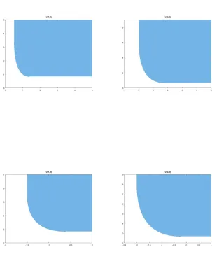
Example 6.5. Let us considerL, U0:R→R2 defined by

L(w) =



 1 2w

2

3 2w

2 

 and U0=

1−w

1 +w

andC=R2+. Some images of the value function are in Figure 1.

Given ζ= (ζ1, ζ2)∈C+\{0}, thenwˆ = ˆw(t, x, ζ)defined in (13) is

ˆ

w=x+tζ1−ζ2 ζ1+ 3ζ2

.

Hypothesis (14) is fulfilled, in fact:

1 tHLζ

_x₋_w_ˆ

t

+HU0,ζ( ˆw) = 1

t(ζ1+ 3ζ2)>0.

Then it is possible to compute (15) and (16):

Ut,ζ(t, x) =

z∈Z

ζ·z≥ −

1 2

(ζ1−ζ2)2

ζ1+ 3ζ2

Uq,ζ(t, x) =

n

z∈Z

ζ·z≥ −(ζ1−ζ2)q o

.

For example for(t, x) = (1,0) and some values ofζ we obtain the following sets:

ζ= (1,0) Ut,ζ(1,0) =

(z1, z2)| z1≥ −1₂

Uq,ζ(1,0) ={(z1, z2)| z1≥ −q}

ζ= (1,1) Ut,ζ(1,0) ={(z1, z2)| z1+z2≥0} Uq,ζ(1,0) ={(z1, z2)| z1+z2≥0}

ζ= (0,1) Ut,ζ(1,0) =

(z1, z2)| z2≥ −1₆

Uq,ζ(1,0) ={(z1, z2)| z2≥q}

The Hamiltonian function is:

Hζ(p) =

\

q∈R

S(p,ζ)(q)−ζL(q)

=

z∈Z | ζ·z≥sup

q∈R

[pq−Lζ(q)]

=

z∈Z | ζ·z≥ p

2

2(ζ1+ 3ζ2)

.

7 Real-valued case

In the particular cased= 1, so when the objective function is real-valued, the value function can be

written as

U(t, x) =u(t, x) +_R+,

where u(t, x) is the classical value function. If the hypotheses hold andu(t, x) is differentiable, it is

easy to see that

Ut,1(t, x) =ut(t, x) +R+,

Uq,1(t, x) =∇u(t, x)·q+R+.

(18)

Hypothesis (14) becomes

1 tL

00

x−wˆ t

+U₀00( ˆw)>0,

since ˆwis a minimizer.

Since

S(p,1)(q) =p·q+R+,

the Hamiltonian function is

H1(p) = sup

q∈Rn

(p·q−L(q)) +_R+

and equations (17) and (18) both become

ut(t, x) +H1

∇L

_x₋_w_ˆ

t

=_R+.

Using (16) and the second equation in (22), the previous equation can be written

ut(t, x) +H1(∇u(t, x)) =R+

and the real-valued case is recovered.

References

[1] _{J.P. Aubin, H. Frankowska,}Set-Valued Analysis,Birkh¨auser, Boston-Basel-Berlin 1990.

[2] R.J. Aumann,Integrals of set-valued functions,J. Math. Anal. Appl.12(1965), 1–12.

[3] E.N. Barron, R. Jensen, W. Liu,Hopf-Lax-type formula for ut+H(u, Du) = 0, Journal of

Differential Equations1261 (1996), 48–61.

[4] _{H. Bonnel, C.Y. Kaya}, Optimization over the efficient set of multi-objective convex optimal control problems, Journal of Optimization Theory and Applications1471 (2010), 93–112.

[5] _{P. Cannarsa, C. Sinestrari,} Semiconcave Functions, Hamilton-Jacobi Equations, and Op-timal Control, Progress in Nonlinear Differential Equations and Their Applications, Birkh¨auser (2004).

[6] _{N. Caroff,}Multicriteria Optimal Control and Vectorial Hamilton-Jacobi Equation,in:

Large-Scale Scientific Computing, LSSC 2007, Eds. I. Lirkov, S. Margenov and J. Wa´sniewski, Lecture

Notes in Computer Science4818, Springer, Berlin, Heidelberg, 293–299.

[7] _{M. Ehrgott,} Multicriteria Optimization, 2nd edition, Springer Science & Business Media (2005).

[8] L.C. Evans,Partial Differential Equations,Graduate Studies in Mathematics 19, Providence, RI, American Mathematical Society (2010).

[9] _{A. G¨}_{opfert, H. Riahi, C. Tammer, C. Zalinescu,}Variational Methods in Partially Ordered Spaces, Springer Science & Business Media (2003).

(19)

[11] _{A.H. Hamel, F. Heyde, A. L¨}_{ohne, B. Rudloff, C. Schrage (Eds.),} Set Optimization and Applications - The State of the Art,Springer Proceedings in Mathematics and Statistics151 (2015).

[12] A.H. Hamel, C. Schrage, Directional derivatives, subdifferentials and optimality conditions for set-valued convex functions,Pacific Journal of Optimization104 (2014), 667–689.

[13] _{N. Katzourakis, T. Pryer,} On Hamilton-Jacobi-Bellman equations arising in deterministic and stochastic optimal control with vectorial cost,arXiv:1409.8648 (2014), 1–18.

[14] _{P.L. Lions,}Generalized Solutions of Hamilton-Jacobi Equations,Research Notes In mathematics

Series69, Pitman Publishing (1982).

[15] _{J. Matkowski, K. Nikodem,}An integral Jensen inequality for convex multifunctions,Results

in Mathematics26 3-4 (1994), 348–353.

[16] _{W. Marks,}Multicriteria optimisation of shape of energy-saving buildings, Building and

Envi-ronment324 (1997), 331–339.

[17] M. Pilecka,Set-valued optimization and its application to bilevel optimization,PhD-thesis 2016,

Technische Universit¨at Bergakademie Freiberg.

[18] R.W. Reid, S.J. Citron,On noninferior performance index vectors, Journal of Optimization

Theory and Applications71 (1971), 11–28.

[19] _{R.B. Vinter,}Optimal Control, Boston, Publisher: Birkhauser (2000).

[20] _{J.J. Wang, Y.Y. Jing, C.F. Zhang, J.H. Zhao,}Review on multi-criteria decision analysis aid in sustainable energy decision-making, Renewable and Sustainable Energy Reviews139 (2009), 2263–2278.

[21] _{P.L. Yu, G. Leitmann,} Nondominated decisions and cone convexity in dynamic multicriteria decision problems, Journal of Optimization Theory and Applications145 (1974), 573–584.

[22] _{P.L. Yu, G. Leitmann,}Compromise solutions, domination structures, and Salukvadze’s

solu-tion, Journal of Optimization Theory and Applications133 (1974), 362–378.

[23] L. Zadeh,Optimality and non-scalar-valued performance criteria, IEEE Transactions on