SPARSE CODED AUTOENCODER FEATURES FOR CHEMOMETRIC DATA ANALYSIS
Muhammad Bilal
1Mohib Ullah
21
University of Trento, Italy.
2
Norwegian University of Science and Technology, Norway.
ABSTRACT
We proposed a deep learning based chemometric data analy-sis technique. We trained L2 regularized sparse autoencoder end-to-end for reducing the size of the feature vector to han-dle the classic problem of curse of dimensionality in chemo-metric data analysis. We introduce a novel technique of auto-matic selection of nodes inside hidden layer of an autoencoder through pareto optimization. Moreover, linear regression, ε-SVR , and Gaussian process regressor are applied on the re-duced size feature vector for the regression. We evaluated our technique on orange juice and wine dataset and results are compared against state-of-the-art methods. Quantitative re-sults are shown on Normalized Mean Square Error (NMSE) and the results show considerable improvement in the state-of-the-art.
Index Terms— Chemometric data,sparse autoencoder, gaussian process regressor, pareto optimization.
1. INTRODUCTION
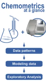
The term chemometric refers to the process of extracting meaningful information from data obtained through a chem-ical experiment [1]. It is a multidisciplinary field of study where techniques from statistical modeling, bayesian infer-ence, deep learning, signal and image processing are applied for data analysis and achieve objective results. Usually, data come from fields like chemistry, Pharmaceutics, bio-chemistry, to name a few. In a nutshell, chemometric consist of three steps:
• Data acquisition
• Descriptive analysis
• Predictive analysis
Chemometric process begins with data acquisition phase. In our experiment, data is obtained through spectroscopy. In spectroscopy, the material under consideration (wine and or-ange juice in our case) is illuminated with a light source of specific wavelength and the reflection and transmission prop-erties are recorded as a function of wavelength. The instru-ment that is used for measuring the intensity of light ray as
Fig. 1: Chemometric analysis in a nutshell.
a function of its wavelength is called photometer. The es-sential characteristics of a spectrophotometer is operational bandwidth, i.e. the range of wavelengths a spectrophotometer is capable of working on the test samples. The the transmis-sion, reflectance and absorption capacities of a test sample are also important parameters. Modern spectrophotometer works in the following four steps:
• The light rays of the desired wavelength are passed through sample under test.
• The incident rays are either transmitted or reflected from the sample.
• The resultant light falls on photodetector device and produces current.
• The current produced is amplified and converted into absorption or transmission values that are later on used for analysis.
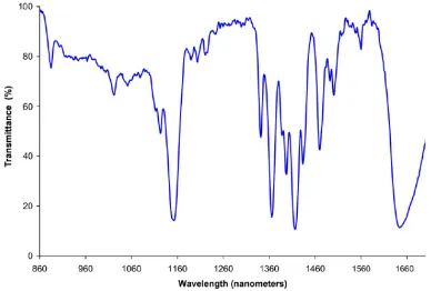
Based on the nature of application, spectroscopic analysis uses different light source like Ultraviolet-Visible (UV-Vis), Infrared (IR), Near Magnetic Resonance (NMR) and X-ray. We will here particularly focus on the IR spectroscopy due to the fact the two datasets for our analysis are collected through IR spectrophotometer.
Fig. 2: Single beam spectrophotometer
Fig. 3: Near-IR absorption spectrum of dichloromethane showing complicated overlapping overtones of mid IR ab-sorption features
1.1. IR spectroscopy
It deals with the effects of interaction of infrared radiation with matter for experimental purposes. Infrared spectrom-eters are used to create infrared spectrum for experimental analysis on the samples, which is basically a graph of in-frared light absorbance or transmittance on vertical axis and frequency or wavelength on horizontal axis, as given in fig.3. The infrared portion of electromagnetic spectrum is fur-ther divided into the following regions;
• Far infrared, with the range 40010cm1
• Mid infrared, with the range 4000400cm1
• Near infrared, with the range 140004000cm1
The mid infrared region is also called FTIR, where FT stands for Fourier Transform. It is called FTIR because to get the actual spectrum a Fourier transform is applied to original raw data that is obtained through FTIR spectrometer. Near in-frared spectroscopy (NIR) has found wide use in applications that are best suited with rapid analyses that allow one to mea-sure a sample in its natural state, as it does not require sample preparation.
Then second and third step of chemometric consist of description and predictive analysis. In descriptive analysis,
properties of chemical systems are modeled for determining the fundamental relationships and structure of the system. While in predictive analysis, properties of chemical systems are modeled for predicting new properties or behavior of interest. In both cases, the datasets can be small but highly complex. Depending on the system requirements and com-plexity levels, the investigative parameters and variables can range from few hundreds to few thousands resulting into a large number of outcomes and case studies. This work is mainly focused on the predictive analysis.
Primarily, the focus is on estimating sugar and alcohol concentration in orange juice and wine. The data is acquired through near infrared (orange juice dataset) and mind infrared (wine dataset) reflectance spectroscopy. The acquired data suffers from the curse of dimensionality. An autoencoder net-work has been designed for reducing the data dimensional-ity and hence addressing this issues. The parameters selec-tion of network is modeled as an optimizaselec-tion problem and pareto optimization is used to get the optimal set of parame-ters. Moreover, three regression models (linear, SVM, Gaus-sian process) have been used to get the estimation on sugar and alcohol concentration.
The paper is organized in the following order. In section 2, related work is elaborated. In the section3, the proposed method is explained. In section4, we present autoencoder training and parameter optimization. The loss function and the training strategies are explained in section5and6, respec-tively. Section7illustrate our baseline regressor. In section8, quantitative results are presented and section9concludes the paper.
2. RELATED WORK
Pre-vious work suggests that existence of such high collinearity between the spectral variables can result in inaccurate pre-dictions [2,3]. It is problematic to apply directly statistical methods due to high collinearity, like multiple linear regres-sion (MLR) in [4–7].
In order to deal with curse of dimensionality and data collinearity, different works have been proposed in literature [8]. Most of the previous work suggests to reduce the number of variables or features to cope with curse of dimensionality problem, thus allowing to get more accurate results through regression techniques. The feature reduction can be gener-ally achieved in two different methods. The first one contains selecting the most relevant features based on a chosen crite-rion from the original set of features [9–12], while in second case the original features are transformed from one space to another in such a way to keep the reconstruction error as mini-mum as possible. This transformation of features set from one space to another can either be linear or non-linear depending upon the scope of application. The examples of later method are Principle Component Regression [13] (PCR) and Partial Least Square Regression (PLSR) [6]. PCR is composed of simple linear regression model based on few principle com-ponents of the original spectral data. While PLSR focuses on calculating the linear projections that shows maximum cor-relation with the output or target variable, thus estimating a linear regression model determined by the projected coordi-nates. Gujral et al. [14] used unlabeled data for reducing the the modeling error. Moreover, an analytic study on a sequen-tial version of Optimal filtering (OF) based PLSR and PCA-based PLSR is conducted and it has been proved analytically that OFbased PLSR is equivalent to that of PCAbased PLSR. Benoudjit et al. [10] proposed linear and nonlinear regres-sion methodologies which are based upon an incremental rou-tine for feature selection and using a validation set. In [11,12], different techniques have been introduced to improve the re-sults of previous method by choosing the best feature set for initializing the routine and finding a feature selection strat-egy that depends entirely on the shared information between spectral data and target variable. An interesting approach to the chemometric problem has been discussed in [15], where instead of traditional feature reduction approach, the whole information in spectral data space is exploited by using Mul-tiple Regression System (MRS). In MRS approach, the esti-mates obtained from a group of regression methods are fused together through a defined mechanism to get the final esti-mate. The results obtained from MRS can be more accurate than single regressor method provided the ensemble is prop-erly designed. The results obtained from MRS technique out-perform the ones obtained through traditional feature reduc-tion techniques such as PCR and PLSR [6,15].
Douak et al. [16] come up with two stage regression ap-proach that is based on residual-based correction (RBC) con-cept. Their basic idea is to correct any adopted regressor, called functional estimator, by analyzing and modeling its
residual errors directly in feature space. RBC is particularly a correction method and not a regressor which does not focuses on achieving the best possible accuracy on the given data set but rather improving the estimation model of the given regres-sion error. In general this proposed technique is suitable for any regression method. The underlying motivation for RBC is that it is typically challenging to acquire a single feature set that is alone capable of giving highly accurate estimates over the total input space. This is due to the fact that the accuracy of the estimator depends on the region of the input space to which the analyzed pattern belongs to.
A semi-supervised approach has been presented in [17], where the unlabeled samples (whose spectral values are known, but the corresponding output concentration values are unknown) are used during the design and configuration of the regressor model in order to counterbalance the deficiency in labeled samples. The advantage in those samples come at no price from the data which is under analysis. Similarly, [18] et al. proposed a semi-supervised Fisher’s linear discriminant analysis (LDA) for projecting the multivariate chemometric data into a lower dimensional space for better data separabil-ity. Consequently, these projections are used to classify test data into different groups.
normalized mean square error as performance indicator for obtaining optimal ELM parameters.
The commonality among existing approaches is, they as-sumed that the training set is composed of sufficient number of training samples in order to obtain accurate estimates of the chemical components of interests through regression tech-niques. However, the process of obtaining training samples through spectroscopic technique is complex and costly. It can be subjected to errors because the concentration measurement is carried out manually by human experts. Consequently, the datasets collected for both training and testing purposes are limited and it possibly affects the performance of the overall estimation process.
The importance of feature reduction and salient fea-tures extraction have been highlighted in other computer vision applications as well like scene understanding [22–24], crowd analysis [25–27], illuminant estimation [28], segmen-tation [29,30], and anomaly detection [31], to name a few. Similarly, In the last few years, deep learning has shown outstanding results on a image classification [32], segmenta-tion [33], and tracking [34,35] etc. Inspired by the success of deep learning in such applications, we proposed an auto-matic deep learning based feature extraction technique. In a nutshell, deep models learns hierarchical features [36,37] and have the capability to learn the structure of the underlying data. We designed an autoencoder neural network [38] for removing redundant and irrelevant features from the spec-tral data. It is an automatic feature extraction technique that is capable of linear and nonlinear feature extraction based upon the selection of parameters of the architecture. Pareto optimization technique is applied in order to choose the best architecture (in terms of model complexity) of autoencoder for the feature extraction. After extracting meaningful fea-tures from the original feature set, we exploited 3 repression techniques (Linear,ε-SVR, and Gaussian process regression) to solved our concentration estimation problem.
3. PROPOSED APPROACH
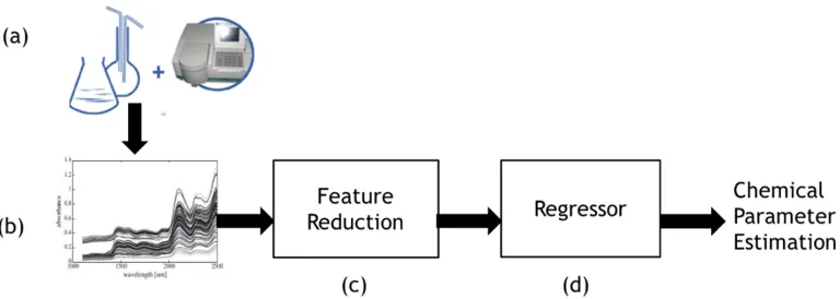
We focus on estimating sugar and alcohol concentration in orange juice and wine datasets. The whole pipeline can be seen in 3 discrete steps. In the first step, date is acquired from the liquids through near infrared (orange juice data set) and mid infrared (wine dataset) reflectance spectroscopy tech-nique Fig. 4 (a,b). In the 2nd step, the acquired data is processed through auto-encoder neural network for feature reduction Fig. 4 (c) and then in the last step, three regres-sion techniques (Gaussian process regressor, linear regressor, SVM regressor) has been used to estimate the concentration of the mentioned components Fig. 4(d). The aim of autoen-coder is to retrieve set of features which are the best represen-tation of original data without redundancy. In a nutshell, the contribution of our work is three folds:
• We proposed a deep learning based framework for au-tomatic chromatic data analysis.
• An autoencoder neural network is designed for address-ing the problem of curse of dimensionality and data collinearity. Moreover, pareto optimization is used to struck the optimal number of parameters in the net-work.
• Three different regressor has been used for estimating the concentration of sugar and alcohol in the datasets and extensive experiments are conducted to validate the proposed scheme.
In the next section4, autoencoder design, the parameter optimization and feature reduction strategy is explained.
4. AUTOENCODER
An autoencoder is a neural network that is trained to recon-struct the input data into the output with minimum amount of reconstruction error. They are designed in a way not to copy the input but to learn important and unique feature of the in-put data. Autoencoders are mainly used for pre-train deep networks dimensionality reduction, feature learning and gen-erative modeling of data. It is composed of two main parts, input layer and output layer together with hidden layer con-necting the two layers. The input layer has the same number of nodes as the output layer. To build an autoencoder we need encoding function at the input, decoding function at the out-put and loss function to calculate the amount of information loss between encoded representation and decoded representa-tion of the input and output data respectively.
4.1. Encoder
It maps an input vectorx∈Rn, into encoded representation
h(x)∈Rm. The typical form is affine mapping followed by
nonlinearity (eq. 1). The parameter set isΘ = (w, b)where wis weight matrix of sizemxnandb∈Rmis bias vector,f
is activation function.
hΘ=f(wx+b) (1)
4.2. Decoder
It maps the resulting encoded representationh(x)back into an estimate of reconstructed n-dimensional vectorr ∈ Rn,
where
rφ=g(f(x)) (2)
Fig. 4: (a) Data collection through spectrophotometry. (b) Spectral signature. (c) Feature reduction through autoencoder neural network. (d) Gaussian process regressor for estimating chemical parameter of interest.
The parameterφ =
w0, b0 , wherew0 is weight matrix of size isnxm,b0∈Rnis bias vector andgis activation func-tion of the decoder. The autoencoder tries to learn a funcfunc-tion rφ'x, thus each training datax(i)is mapped to correspond-ing reconstructed datar(i). By forcing the number of hidden nodes lower than the dimension of the input data, the autoen-coder tries to learn representative structure of the data or by imposing sparsity constraint on the hidden nodes the autoen-coder learns useful features even for hidden nodes equal or higher than the input dimension. For a given N training sam-ples the autoencoder learns to minimize the loss function eq. 5such as mean squared reconstruction error by optimizing the model parametersΘandΩeq.4
Θ,Ω = arg min Θ,Ω
L(x, r) (4)
L= 1 N
N
X
n=1
(xi−ri)2 (5)
4.3. Regularized autoencoder
In order to have a flexible model independent of the size of the hidden nodes and capability of the activation functions on the other hand that relies on the complexity of distribution of the data is an ideal condition. To achieve this, we introduce ad-ditional regularization parameters to the loss function, mainly sparsity of representation and smallness of the derivative of the representation (weight decay).
4.3.1. Regularizing by weight decay (L2 regularization)
To avoid overfitting - a problem where a model memorizes training data but not able to generalize when it is given unseen data leading to performance decline in the model, the rate in which the model reacts to changes in the training example distribution is penalized by forcing the autoencoder to learn
most significant features.
Ωweights= 1 2
L
X
l N
X
j K
X
i
(wlij))2 (6)
whereLthe number of hidden layers is,N is the number of training examples andKis the number of features.
4.4. Sparse autoencoder
Typical use of sparse Autoencoders is to learn features for the purpose of classification or regression. Imposing spar-sity constraint on the hidden nodes enables the model to learn unique statistical features of the data even when the number of hidden units are larger compared to the feature space of the input data. A neuron is considered active if its output value is close to maximum value of the activation function used (close to 1 for sigmoid activation function) and inactive if its output is close to minimum value (0 in case of sigmoid). The average activation ofithhidden unitρˆ
ieq.7, where n is total number of inputs,xj is thejthtraining example andhi activation of jthhidden unit is given as:
ˆ ρi = 1
n n
X
j=1
hi(xj) (7)
Ωsparsity= m
X
i=1
KL(ρ||ρi)ˆ (8)
Choosing sparsity parameterρsmall (ρ=0.01) and impos-ingρiˆ = ρconstraint, Kullback-Leibler divergence term is applied to penalizeρi. Penalty value that diverges fromˆ ρwill give reasonable result.
KL(ρ||ρi) =ˆ ρlog(ρ ˆ ρi
) + (1−ρ) log(1−ρ 1−ρˆi
) (9)
random variable with meanρi. Ifˆ ρ = ˆρi,KL(ρ||ρi) = 0,ˆ else increases monotonically asρiˆ diverges fromρ. Minimiz-ing theKLdivergence penalty term leads toρˆito be close to ρ.
5. LOSS FUNCTION
Imposing sparsity constraint on the hidden nodes of an au-toencoder enables the model to learn unique statistical fea-tures of the data even when the number of hidden units are larger compared to the feature space of the input data. A neu-ron is considered active if its output value is close to maxi-mum value of the activation function used (close to 1 for sig-moid activation function) and inactive if its output is close to minimum value (0 in case of sigmoid). The average activa-tion ofithhidden unitρiˆ is given in eq. 7, wherenis total number of inputs,xj is thejthtraining example andhi acti-vation ofjthhidden unit. The combining all the components, the synergetic loss function can be written as:
L(Θ,Ω) = 1 N N X n=1 K X k=1
(xkn−rkn)2+λ∗Ωweights+β∗Ωsparsity
(10) whereΩsparsity is sparsity regularizer and calculated as eq. 8: Similarly, Ωweights is L2 regularization term. It’s task is to avoid overfitting by penalizing the rate in which the model reacts to changes in the training example distribution and forcing the model to learn most significant features. It is calculated as eq.11
Ωweights= 1 2 L X l N X j K X i (wlij))
2
(11)
where L is number of hidden layers, N is the number of training examples andK is the number of features. In the lost function,λis coefficient for theL2regularization term, Ωweights andβ is the coefficient for sparsity regularization Ωsparsityterm.
6. TRAINING
Once the model is setup, our goal is to minimize the cost func-tionL(Θ,Ω)as a function of weightswand biasb. To train our autoencoder neural network, we initialized each parame-terw(l)i,j,andb(l)i to a small random value near zero(N(0, ε2) distribution for a smallε)), and then apply stochastic conju-gate gradient decent (SCG) algorithms to learn the network parameters of autoencoder. Random initialization is neces-sary, if all the parameters start off at identical values, then all the hidden layer units will end up learning the same function of the input.
SCG minimizes network parameters by taking steps in negative direction of the loss function. Starting with initial set
of parameter values, the algorithm iteratively approaches to-wards a set of parameters values that minimize the loss func-tion. Back-propagation is used to compute the derivative of the loss function with respect to network parameters. A loss function that penalizes for estimatingrinstead of x, gradi-ent decgradi-ent algorithm iteratively updates network parameter (weights and biases) in such a way that the reconstruction error at the output is minimized. A single iteration of SCG updates the parametersw,bas (eq. 12) and (eq. 13) respec-tively.
w(l)ij =w(l)ij −ζ ∂ w(l)ij
L (12)
b(l)i =b(l)i −ζ ∂ b(l)i
L (13)
Whereζis learning rate andLis the loss function. The partial derivatives of the loss function L(w, b;x, r)defined with respect to a single example(x, r)is given by (eq. 14) and (eq.15) respectively.
∂ w(ijl)
L=
1 N
PN i=1w∂(l)
ij
L(w, b;x(i), r(i))
+λwij(l)+β−ρρˆi+11+ ˆ−ρρ
(14)
∂ b(l)i
L= 1 N
N
X
i=1 ∂ w(l)ij
L(w, b;x(i), r(i)) (15)
Back-propagation is used to efficiently compute these par-tial derivatives. Given a training examplex, we will first run a forward pass to compute all the activations throughout the network, including the output value of the reconstructionr. Then, for each nodeiin layerl, we would like to compute an error termδi(l)that measures how much that node was re-sponsible for any errors in our output. For an output node, we can directly measure the difference between the network’s activation and the true target value, and use that to define δi(nl)(where layernlis the output layer). For hidden units we computeδi(l)based on a weighted average of the error terms of the nodes that useshi(l)as an input. In Back-propagation algorithm, first perform a feed-forward pass computing the activation of all layers starting from the first hidden layer to the output layernl, then for each output unitiin layernlthe error value is given by (eq.16).
δ(nl)=−(x−r)∗g0(h(nl)) (16)
δl= (wl)Tδl+1∗g0(h(l)) l=nl−1, nl−2, ...,2 (17)
For the hidden layers, the error is given by equation16, and the desired partial derivatives are given by (eq. 18) for weight update and (eq.19) for the bias term update.
∇b(l)L=δl+1 (19) wheregis activation function at a given layer. By repeat-edly taking conjugate gradient decent steps it minimizes the loss functionL.
6.1. Optimization
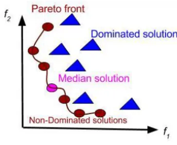
The choice on model complexity and mean squared error (MSE) are two trade-offs to optimize the loss function. As we increase the number of hidden nodes MSE decreases. However, the increase in the number of hidden-neurons might lead to overfitting the data, thus decreasing the generalization performance of the model. The goal is to find an optimal solution for both model complexity and MSE that maxi-mizes the model performance. We exploited Pareto Based Multi Objective Learning(PMOL) for estimating the optimal number of parameters for our autoencoder. It uses vector of objective functions and therefore number of optimal solutions are more than one. Pareto front of optimal solution is a set of non-dominated solutions, being chosen as optimal, if no objective can be improved without sacrificing at least one other objective. On the other hand a solutionX is referred to as dominated by another solutionY if, and only if,Y is equally good or better thanX with respect to all objectives. Pareto based multi object optimization can be formulated as eq.20withQobjective functions;
f(p) = [fi(p), i= 1, ..., Q] (20) subjected to the equality constraints
gj(p) = 0 j = 1,2, ..., J (21) And the K inequality constraints
hk(p)≤0 k= 1,2, ..., K (22)
The aim is to find vectorp∗which minimizesf(p), in our case since we have two objective function thus pareto based bi-objective learning problem can be formulated to minimize the two objectives, that is data fitting term and model com-plexity term given by eq.23
f1=−L(E|Θ), f2=γklog(L) (23) wheref1 = −L(E|Θ) is data fitting objective function andf2 =γklog(L)is model complexity objective function. f1 is log-likelihood function that is found with a maximum likelihood estimation algorithm.E= (ε1, ε2, ...εL)is a set of multi-dimensional reconstruction error. Assuming the error is multivariate normal distribution with Mean vectorM = 0and covarianceΣ, then the distribution function is given by:
p(ε) =N(M,Σ) = 1 2πq|Σn2
f|
exp(−1
2ε
TΣ−1ε) (24)
Fig. 5: Pareto front and the median solution
where the negative log-likelihood function will be repre-sented by
−L(E|Θ) = log L
Y
i=1
p(εi) (25)
Assuming the features are identically independently dis-tributed (iid), the covariance matrixΣis given by;
Σ =
Ω2
1 0 0 . . . 0 0 Ω2
2 0 . . . 0 0 0 Ω2
3 . . . 0 . . . .
0 0 0 . . . Ω2 n
γis a constant determined by a pareto optimizer,Lis input training sample size, k is the number of parameters of the model to be estimated (weight and bias). Ωis the standard deviation.
Pareto-based multi objective learning algorithms are able to achieve a number of Pareto-optimal solutions, from which the user is able to extract knowledge about the problem and make a better decision when choosing the final solution. Once the pareto front optimal solutions are found, one optimal so-lution can be chosen using different methods for example the average, median etc. In this paper, we use median value as an optimal solution as shown in the fig.5.
7. REGRESSION TECHNIQUES
Statistical regression is basically a way to predict unknown quantities from a batch of existing data. In all regression tech-niques the aim is to find ’the best’ function that is estimated over training samples(X1, y1),(Xn, yn)in order to predict y given X, where X ∈ Rd andy ∈ R. In our work, we
have used the following three regression techniques for pre-dicting the concentration of chemical component of interest in the given data sets.
Fig. 6: Near-infrared spectra of orange juice training samples
• support vector regression (SVR)
• Gaussian process regression (GPR)
A detailed description of regression techniques is beyond the scope of this paper. Interested readers may refer to [39]. GPR worked well for our application because our data is non-linear and it fits very well for our problem.
8. EXPERIMENTS 8.1. Dataset description
In this work we have used two spectrophotometric datasets, coming from the food industry. The first dataset deals with determining sugar content in the orange juice sample by near infrared reflectance spectrometry [40]. The training and test samples in the orange juice data are 149 and 67 respectively; with 700 spectral variables that represents the absorbance (log 1/R) between 1100nm and 2500nm. The value of R represents light reflected by the sample. The concentration of sugar ranges from 0%to 95.2%by weight in the sample. The spectra of orange juice obtained from the training set is shown in fig6.
The second dataset deals with the determination of al-cohol content by mid-infrared spectroscopy in wine samples [40]. The training and test data sets contain 91 and 30 spec-tra, respectively, with 256 spectral variables that are the ab-sorbance (log 1/T) at 256 wave numbers between 4000 and 400 cm−1 (where T is the light transmittance through the sample thickness). Alcohol content varies from 7.48% to 15.5%by volume. No preprocessing has been performed on the orange juice and wine datasets.
8.2. Estimation Error Assessment
For the quantitative results, the accuracy of the approach is represented in normalized mean square error (NMSE) metric,
Methods Orange juice Wine
Douak et al. [16] 01574 0.0070
Benoudjit et al. [15] 0.2435 0.0052
Alhichri et al. [21] 0.32076 0.0034
Ours 0.1711 0.0042
Table 1: Quantitative results of our method against 3 state-of-the-art methods. Numeric values shows Normalized Mean Square Error (NMSE), the lower is NMSE, the better is per-formance.
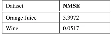
Dataset NMSE
Orange Juice 5.3972
Wine 0.0517
Table 2: NMSE achieved on orange juice and wine dataset using all feature by linear regressor
which is define as:
N M SE= 1 Vtrain+test
M
X
i=1
(yitest−y0itest)2 (26)
whereM represents the number of testing samples,yitest andy0itestare the real and estimated outputs for theith test samplexitestandVtrain+testis the combined variance of the training and test output samplesyitrainandyitest.
8.3. Quantitative results
An extensive experiments are conducted to validate our ap-proach. Initially, we used all the spectral features for both he datasets. Later, we used different number of features ex-tracted through autoencoder neural networks for estimating the sugar and alcohol concentration in the samples.
8.3.1. All features
This section report the results obtained from different regres-sors by using ALL-features (original hyper dimensional input space), that is, 700 and 256 features for orange juice and wine data set, respectively.
Dataset Kernel type NMSE
Orange juice linear 0.1905
Orange juice radial basis function 0.1820
wine linear 0.0039
wine radial basis function 0.0038
Table 3: NMSE achieved on orange juice and wine dataset using all feature byε-SVR
Kernel function Basis function
Orange juice
Wine
Squared exponential constant 0.1316 0.0041
matern32 constant 0.1244 0.0038
matern32 constant 0.1313 0.0041
Squared exponential linear 5.3972 0.0517
matern32 linear 5.3972 0.0517
matern32 linear 5.3972 0.0517
Table 4: NMSE achieved on orange juice and wine dataset using all feature by GPR
Parameter for orange juice:
• Linear: C = 183.29,ε=10−2
• Radial Basis Function: C= 103,ε=103,γ= 0.3
Parameter for wine:
• Linear: C =103,ε=10−2
• Radial Basis Function: C=103,ε=10−2,γ= 0.15
8.3.2. Deep features through autoencoder
This section report the results obtained from three regressors using features that extracted through autoencoder neural net-work. The number of hidden units used in the autoencoder architecture are 2, 5, 10, 20,..., 200 with an increment value of 10 between 10 and 200 nodes. The encoder and decoder transfer functions used are ’satlin’ [41] and ’logsig’ [42].
Orange juice dataset
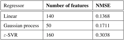
For the orange juice dataset, 700 spectral features are reduced to 2, 5, 10, 20,..., 200 features, with an increment value of
Regressor Number of features NMSE
Linear 140 0.1368
Gaussian process 50 0.1711
ε-SVR 160 0.3038
Table 5: NMSE achieved on orange juice dataset using deep feature
10. The extracted features (2, 5, 10, 20,..., 200 with an in-crement value of 10) of 149 training samples are used one by one to train the regression model of Linear, Gaussian process and support vector regressors. For testing, 67 samples from test data set is used and the performance of each regressor is shown in terms of normalized means square error NMSE value. In table5, the best NMSE values achieved on three regressors are reported.
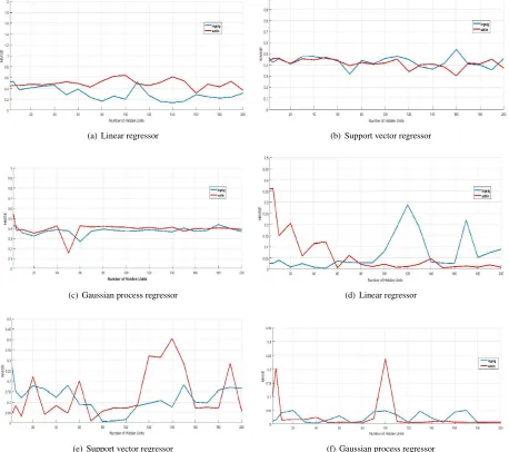
In case of GPR, the square exponential kernel function is adopted with ’constant’ basis function. For SVR, the re-sult reported in table5is achieved using ’radial basis func-tion’. kernel function with regularization parameter C = 103, ε = 10−2and kernel widthγ= 0.1. In particular, C, γand εwere varied from10−4to103, from10−4to103and from 10−4to10−1, respectively. The result obtained using linear kernel function is quiet close to the one reported in table5, which is NMSE = 0.3084. In fig.7(a-c), we demonstrate the varying behavior of NMSE over different hidden units used in autoencoder during feature extraction process for all the three regressors.
In case of linear regressor, the performance achieved us-ing ’logsig’ activation function for hidden units or nodes in encoder and decoder of autoencoder is more consistent and better than the one achieved used ’satlin’, as number of hid-den nodes increases. While for GPR and SVR, the behavior of NMSE achieved using ’logsig’ and ’satlin’ activation func-tions is consistent and more stable over the set of hidden units chosen for the feature extraction through autoencoder.
8.3.3. Autoencoder parameter optimization for orange juice
(a) Linear regressor (b) Support vector regressor
(c) Gaussian process regressor (d) Linear regressor
(e) Support vector regressor (f) Gaussian process regressor
Fig. 8: Pareto dominance for orange juice dataset
Regressor Number of hid-den units in first layer
NMSE using 1 hidden layer
Number of hid-den units in second layer
NMSE using 2 hidden layers
Linear 140 0.1368 100 0.3086
Gaussian process
50 0.1711 150 0.4098
ε-SVR 160 0.3038 100 0.4059
Table 6: Comparison of best NMSEs achieved using one and two hidden layers for orange juice dataset
indicating increasing the hidden layer have negative effect in the model. This is due to the fact that we already selected an optimal number of hidden units in the first layer that best represents the network architecture.
8.3.4. Wine dataset
In wine dataset, the number of spectral features are 256 which are less as compare to the ones in orange juice dataset. Like orange juice dataset experiment, the extracted features (2, 5, 10, 20,..., 200 with an increment value of 10) of 91 training samples are used one by one to train the regression model of Linear, Gaussian process and support vector regressors. For testing, 30 samples from test data set is used and the per-formance of each regressor is shown in terms of normalized means square error NMSE value. In table7, the best NMSE values achieved on three regressors are reported.
In fig. 7(d-f), we demonstrate the varying behavior of NMSE over different hidden units used in autoencoder dur-ing feature extraction process for all the three regressors.
Regressor Number of features NMSE
Linear 50 0.0039
Gaussian process 40 0.0042
ε-SVR 80 0.0075
Table 7: NMSE achieved on wine dataset using deep feature
Regressor Number of hid-den units in first layer
NMSE using 1 hidden layer
Number of hid-den units in second layer
NMSE using 2 hidden layers
Linear 50 0.0039 30 0.0035
Gaussian process
40 0.0043 30 0.0137
ε-SVR 80 0.0075 100 0.0241
Table 8: Comparison of best NMSEs achieved using one and two hidden layers for wine dataset
8.3.5. Autoencoder parameter optimization for wine dataset
Just like orange dataset, we did quantitative analysis through deep learning by using 2 hidden layers (stacked AE). From table 11, the overall NMSE decrease comparing to the values obtained using single layer for GPR and SVR, indicating in-creasing the hidden layer have negative effect on the model. This is due to the fact that we already selected an optimal number of hidden units in the first layer which represents the network architecture optimally.
To determine the optimal number of hidden nodes in the network, we use pareto dominance optimization technique to optimizes the trade-off between number of hidden nodes and model complexity as we did for the orange juice dataset. The fig.9shows a plot of dominated and non-dominated solution using pareto dominance technique for wine data.
It can be seen from Table5and7that in contrast to the concentration of alcohol in the wine samples, the estimation of sugar concentration appears more difficult despite a larger number of spectral data and training samples. This is due to high nonlinearity of the spectral signature of this chemical component.
8.4. Comparsion with state-of-the-art
Fig. 9: Pareto dominance for wine dataset
Regressor methods
NMSE values for orange juice dataset
NMSE values for wine dataset
PLSR 0.161 0.0053
RBFN 0.1574 0.007
SVM 0.2497 0.0081
Table 9: NMSE values achieved on 3 regression methods im-plemented with residual based correction (RBC) [16]
9. CONCLUSION
We propose a novel deep learning based chemometric data analysis technique for estimating sugar and alcohol concen-tration in orange juice and wine samples. L2 regularized sparse autoencoder is trained end-to-end for reducing the size of the feature vector to handle the classic problem of curse of dimensionality in chemometric data analysis. The optimal set of parameters of the autoencoder are selected through pareto optimization. Three regressor namely, Gaussian process, sup-port vector and linear regressor are applied on the reduced size feature vector for estimating the concentration of sugar and alcohol in the corresponding samples. Extensive quan-titative analysis are conducted with different configuration and the results are compared with state-of-the-art methods. Quantitative results are shown on Normalized Mean Square Error (NMSE) and our approach shows better results on both datasets.
10. REFERENCES
[1] Svante Wold, “Chemometrics; what do we mean with it, and what do we want from it?,”Chemometrics and Intelligent Lab-oratory Systems, vol. 30, no. 1, pp. 109–115, 1995.
[2] Jon M Sutter and John H Kalivas, “Comparison of forward selection, backward elimination, and generalized simulated an-nealing for variable selection,”Microchemical journal, vol. 47, no. 1-2, pp. 60–66, 1993.
Regressor methods
NMSE values for orange juice dataset
NMSE values for wine dataset
Linear 0.1368 0.0039
GPR 0.1711 0.0042
ε-SVR 0.3038 0.0075
Table 10: NMSE values for both datasets using number of extracted features suggested by pareto optimization.
[3] Dominique Bertrand, “La spectroscopie proche infrarouge et ses applications dans les industries de lalimentation animale,”
Productions Animales 3 (15), 209-219.(2002), 2002.
[4] David A Belsley, Edwin Kuh, and Roy E Welsch, Regres-sion diagnostics: Identifying influential data and sources of collinearity, vol. 571, John Wiley & Sons, 2005.
[5] Tomas Ekl¨ov, Per M˚artensson, and Ingemar Lundstr¨om, “Se-lection of variables for interpreting multivariate gas sensor data,”Analytica Chimica Acta, vol. 381, no. 2-3, pp. 221–232, 1999.
[6] Paul Geladi, “Some recent trends in the calibration literature,”
Chemometrics and Intelligent Laboratory Systems, vol. 60, no. 1-2, pp. 211–224, 2002.
[7] Harald Martens and Paul Geladi,Multivariate calibration, Wi-ley Online Library, 1989.
[8] Michel Verleysen et al., “Learning high-dimensional data,” 2003.
[9] John A Cornell, “Classical and modern regression with appli-cations,” 1987.
[10] Nabil Benoudjit, E Cools, Marc Meurens, and Michel Ver-leysen, “Chemometric calibration of infrared spectrometers: selection and validation of variables by non-linear models,”
Chemometrics and Intelligent Laboratory Systems, vol. 70, no. 1, pp. 47–53, 2004.
[11] Nabil Benoudjit, Damien Franc¸ois, Marc Meurens, and Michel Verleysen, “Spectrophotometric variable selection by mutual information,” Chemometrics and Intelligent Laboratory Sys-tems, vol. 74, no. 2, pp. 243–251, 2004.
[12] Fabrice Rossi, Amaury Lendasse, Damien Franc¸ois, Vincent Wertz, and Michel Verleysen, “Mutual information for the se-lection of relevant variables in spectrometric nonlinear mod-elling,”Chemometrics and intelligent laboratory systems, vol. 80, no. 2, pp. 215–226, 2006.
[13] Svante Wold, Kim Esbensen, and Paul Geladi, “Principal com-ponent analysis,”Chemometrics and intelligent laboratory sys-tems, vol. 2, no. 1-3, pp. 37–52, 1987.
Regressor methods
NMSE values for orange juice dataset
NMSE values for wine dataset
PCR 0.2596 0.003
PLSR 0.2435 0.0052
VW-PLS 0.2315 0.0031
MRS with lin-ear regressors (AFS)
0.2334 0.0038
MRS with lin-ear regressors (WFS)
0.2354 0.0033
MRS with lin-ear regressors (NLFS)
0.1461 0.0030
MRS with RBFN re-gressors (AFS)
0.3123 0.0038
MRS with lin-ear regressors (WFS)
0.1806 0.0028
MRS with lin-ear regressors (NLFS)
0.1742 0.0026
Table 11: Results achieved on both the wine and orange juice datasets by three reference regression methods and proposed MRS approach implemented with UPS technique [15]
[15] N Benoudjit, F Melgani, and H Bouzgou, “Multiple regression systems for spectrophotometric data analysis,” Chemometrics and Intelligent Laboratory Systems, vol. 95, no. 2, pp. 144– 149, 2009.
[16] F Douak, N Benoudjit, and F Melgani, “A two-stage regression approach for spectroscopic quantitative analysis,” Chemomet-rics and Intelligent Laboratory Systems, vol. 109, no. 1, pp. 34–41, 2011.
[17] Xiaojin Zhu, “Semi-supervised learning literature survey,” 2005.
[18] Deirdre Toher, Gerard Downey, and Thomas Brendan Mur-phy, “Semi-supervised linear discriminant analysis,” Journal of Chemometrics, vol. 25, no. 12, pp. 621–630, 2011. [19] Burr Settles, “Active learning literature survey. 2010,”
Com-puter Sciences Technical Report, vol. 1648.
[20] Fouzi Douak, Farid Melgani, Naif Alajlan, Edoardo Pasolli, Yakoub Bazi, and Nabil Benoudjit, “Active learning for spec-troscopic data regression,” Journal of Chemometrics, vol. 26, no. 7, pp. 374–383, 2012.
Regressor meth-ods
NMSE values for orange juice dataset
NMSE values for wine dataset
Fusion average 0.31978 0.00329
WCS 0.31844 0.00277
IOWA 0.1355 0.00265
Table 12: Results for orange juice and wine datasets [21]
[21] Haikel AlHichri, Yakoub Bazi, Naif Alajlan, Farid Melgani, Salim Malek, and Ronald R Yager, “A novel fusion approach based on induced ordered weighted averaging operators for chemometric data analysis,” Journal of Chemometrics, vol. 27, no. 12, pp. 447–456, 2013.
[22] Habib Ullah and Nicola Conci, “Crowd motion segmentation and anomaly detection via multi-label optimization,” inICPR workshop on pattern recognition and crowd analysis, 2012.
[23] Habib Ullah and Nicola Conci, “Structured learning for crowd motion segmentation,” in2013 IEEE International Conference on Image Processing. IEEE, 2013, pp. 824–828.
[24] Mohib Ullah, Habib Ullah, Nicola Conci, and Francesco GB De Natale, “Crowd behavior identification,” in2016 IEEE International Conference on Image Processing (ICIP). IEEE, 2016, pp. 1195–1199.
[25] Habib Ullah, Muhammad Uzair, Mohib Ullah, Asif Khan, Ayaz Ahmad, and Wilayat Khan, “Density independent hy-drodynamics model for crowd coherency detection,” Neuro-computing, vol. 242, pp. 28–39, 2017.
[26] Paolo Rota, Habib Ullah, Nicola Conci, Nicu Sebe, and Francesco GB De Natale, “Particles cross-influence for en-tity grouping,” in21st European Signal Processing Conference (EUSIPCO 2013). IEEE, 2013, pp. 1–5.
[27] Habib Ullah,Crowd Motion Analysis: Segmentation, Anomaly Detection, and Behavior Classification, Ph.D. thesis, Univer-sity of Trento, 2015.
[28] Fawad Ahmad, Asif Khan, Ihtesham Ul Islam, Muhammad Uzair, and Habib Ullah, “Illumination normalization using independent component analysis and filtering,” The Imaging Science Journal, vol. 65, no. 5, pp. 308–313, 2017.
[29] Habib Ullah, Mohib Ullah, and Muhammad Uzair, “A hybrid social influence model for pedestrian motion segmentation,”
Neural Computing and Applications, pp. 1–17, 2018.
[30] Habib Ullah, Mohib Ullah, and Nicola Conci, “Dominant mo-tion analysis in regular and irregular crowd scenes,” in Interna-tional Workshop on Human Behavior Understanding. Springer, 2014, pp. 62–72.
[31] Habib Ullah, Ahmed B Altamimi, Muhammad Uzair, and Mo-hib Ullah, “Anomalous entities detection and localization in pedestrian flows,”Neurocomputing, vol. 290, pp. 74–86, 2018.
impact of residual connections on learning,” inThirty-First AAAI Conference on Artificial Intelligence, 2017.
[33] Mohib Ullah, Ahmed Mohammed, and Faouzi Alaya Cheikh, “Pednet: A spatio-temporal deep convolutional neural network for pedestrian segmentation,” Journal of Imaging, vol. 4, no. 9, pp. 107, 2018.
[34] Mohib Ullah and Faouzi Alaya Cheikh, “Deep feature based end-to-end transportation network for multi-target tracking,” in
IEEE International Conference on Image Processing (ICIP), 2018, pp. 3738–3742.
[35] Mohib Ullah and Faouzi Alaya Cheikh, “A directed sparse graphical model for multi-target tracking,” inIEEE Conference on Computer Vision and Pattern Recognition Workshops, 2018, pp. 1816–1823.
[36] Mohib Ullah, Ahmed Kedir Mohammed, Faouzi Alaya Cheikh, and Zhaohui Wang, “A hierarchical feature model for multi-target tracking,” inIEEE International Conference on Image Processing (ICIP), 2017, pp. 2612–2616.
[37] Habib Ullah, Muhammad Uzair, Arif Mahmood, Mohib Ullah, Sultan Daud Khan, and Faouzi Alaya Cheikh, “Internal emo-tion classificaemo-tion using eeg signal with sparse discriminative ensemble,”IEEE Access, vol. 7, pp. 40144–40153, 2019.
[38] Pierre Baldi, “Autoencoders, unsupervised learning, and deep architectures,” inProceedings of ICML Workshop on Unsuper-vised and Transfer Learning, 2012, pp. 37–49.
[39] Carl Edward Rasmussen, “Gaussian processes in machine learning,” inAdvanced lectures on machine learning, pp. 63– 71. Springer, 2004.
[40] Marc Meurens, “Spectrophotometric samples of orange juice and wine for chemometric analysis,” .
[41] HK Chang and WA Chien, “Neural network with multi-trend simulating transfer function for forecasting typhoon wave,”
Advances in Engineering Software, vol. 37, no. 3, pp. 184–194, 2006.

![Table 9: NMSE values achieved on 3 regression methods im-plemented with residual based correction (RBC) [16]](https://thumb-us.123doks.com/thumbv2/123dok_us/8014177.1332507/12.612.315.558.71.161/table-values-achieved-regression-methods-plemented-residual-correction.webp)
