https://doi.org/10.5194/nhess-18-383-2018 © Author(s) 2018. This work is distributed under the Creative Commons Attribution 4.0 License.
Automatic detection of snow avalanches in continuous seismic
data using hidden Markov models
Matthias Heck1, Conny Hammer2, Alec van Herwijnen1, Jürg Schweizer1, and Donat Fäh2
1WSL Institute for Snow and Avalanche Research SLF, Davos, Switzerland 2Swiss Seismological Service (SED), ETH Zurich, Zurich, Switzerland
Correspondence:Matthias Heck ([email protected]) Received: 20 June 2017 – Discussion started: 10 July 2017
Revised: 21 November 2017 – Accepted: 2 December 2017 – Published: 25 January 2018
Abstract.Snow avalanches generate seismic signals as many other mass movements. Detection of avalanches by seis-mic monitoring is highly relevant to assess avalanche dan-ger. In contrast to other seismic events, signals generated by avalanches do not have a characteristic first arrival nor is it possible to detect different wave phases. In addition, the moving source character of avalanches increases the in-tricacy of the signals. Although it is possible to visually detect seismic signals produced by avalanches, reliable au-tomatic detection methods for all types of avalanches do not exist yet. We therefore evaluate whether hidden Markov models (HMMs) are suitable for the automatic detection of avalanches in continuous seismic data. We analyzed data recorded during the winter season 2010 by a seismic ar-ray deployed in an avalanche starting zone above Davos, Switzerland. We re-evaluated a reference catalogue contain-ing 385 events by groupcontain-ing the events in seven probability classes. Since most of the data consist of noise, we first ap-plied a simple amplitude threshold to reduce the amount of data. As first classification results were unsatisfying, we an-alyzed the temporal behavior of the seismic signals for the whole data set and found that there is a high variability in the seismic signals. We therefore applied further post-processing steps to reduce the number of false alarms by defining a min-imal duration for the detected event, implementing a voting-based approach and analyzing the coherence of the detected events. We obtained the best classification results for events detected by at least five sensors and with a minimal duration of 12 s. These processing steps allowed identifying two pe-riods of high avalanche activity, suggesting that HMMs are suitable for the automatic detection of avalanches in seismic data. However, our results also showed that more sensitive
sensors and more appropriate sensor locations are needed to improve the signal-to-noise ratio of the signals and therefore the classification.
1 Introduction
During the winter season, snow avalanches may threaten people and infrastructure in mountainous regions through-out the world. Avalanche forecasting services therefore reg-ularly issue avalanche bulletins to inform the public about the avalanche conditions. Such an avalanche forecast re-quires meteorological data, information about the snow-pack and avalanche activity data. The latter are mostly ob-tained through visual observations requiring good visibility. Avalanche activity data are therefore often lacking during periods of intense snowfall, which are typically the periods when they are most important for forecasting. A possible al-ternative approach to determine the avalanche activity is to use a seismic monitoring system (e.g., van Herwijnen and Schweizer, 2011a).
earth-quakes or nearby blasts. A more in-depth analysis of seis-mic signals generated by avalanches was performed 20 years later, identifying typical characteristics in both the time and time–frequency domain (Kishimura and Izumi, 1997; Sabot et al., 1998). Using automatic cameras to film avalanches, (Sabot et al., 1998) showed that specific features in the seis-mic signals were related directly to changes in the flow of the avalanche; these findings were confirmed by (Suriñach et al., 2000) and (Suriñach et al., 2001). Since then, seismic signal characteristics were used to estimate specific properties of single avalanches such as the flow velocity (Vilajosana et al., 2007a), the total energy of the avalanche (Vilajosana et al., 2007b) or the runout distance (Pérez-Guillén et al., 2016; van Herwijnen et al., 2013).
While many studies focused on using seismic signals to better understand the properties of single avalanches, con-tinuous monitoring of avalanche starting zones to obtain more accurate avalanche activity data is of particular interest for avalanche forecasting (e.g., van Herwijnen et al., 2016). (Leprettre et al., 1996) deployed three-component seismic sensors at two different field sites and compared seismic sig-nal characteristics to a database including avalanches, heli-copters, thunder rolls and earthquakes. (Lacroix et al., 2012) improved the seismic monitoring system used by (Leprettre et al., 1996) by deploying a seismic array between two known avalanche paths. The array consisted of six vertical nent geophones arranged in a circle around a three compo-nent geophone in the center. Using array techniques, (Lacroix et al., 2012) determined the release area and the path of man-ually identified avalanches and estimated their speed. These studies mainly monitored medium and large avalanches. Van Herwijnen and Schweizer (2011) however, deployed seis-mic sensors near an avalanche starting zone above Davos in the eastern Swiss Alps to also detect small avalanches. They manually identified several hundred avalanche events in the continuous seismic data during 4 winter months.
While these studies have highlighted the usefulness of seismic monitoring to obtain more accurate and complete avalanche activity data, using machine learning algorithms to automatically detect snow avalanches has thus far remained relatively unsuccessful. Nevertheless, the interest in these techniques has been evident for several decades (Leprettre et al., 1998; Bessason et al., 2007; Rubin et al., 2012). The first attempt to automatically detect avalanches focused on using fuzzy logic rules and credibility factors derived from features of the seismic signal in the time and time–frequency domain (Leprettre et al., 1996, 1998). In a first step, the fea-tures of unambiguously identified seismic events were an-alyzed including avalanches, blast and teleseismic events. They then formulated several fuzzy logic rules for each type of event to train a classifier used to identify the type of a new unknown seismic event. While the probability of detection (POD), i.e., the number of detected avalanches divided by the total number of observed avalanches, was high (≈90 %), one of the main drawbacks of this method is the subjective
expert knowledge used to derive the fuzzy logic rules and the need to adapt these rules to each individual field site.
(Bessason et al., 2007) deployed seismic sensors in sev-eral known avalanche paths along an exposed road in Iceland. They used a nearest-neighbor method to automatically iden-tify avalanche events. The method consists of comparing new events with those in a database. Although a 10-year database was used, the identification performed rather poorly. Seismic signals generated by rockfalls and debris flows were wrongly classified as avalanches and vice versa, resulting in a POD of about 65 %.
In an attempt to improve the automatic detection of avalanches, (Rubin et al., 2012) used a seismic avalanche cat-alogue presented by (van Herwijnen and Schweizer, 2011b) and compared the performance of 12 different machine learn-ing algorithms. The PODs of all classifiers were high (be-tween 84 and 93 %). However, the main drawback were the high false alarm rates, much too high for operational tasks.
The methods described above are generally difficult to ap-ply at new sites since they require time to build a training data set and/or expert knowledge to define thresholds and rules. To overcome these drawbacks, we investigate using a hid-den Markov model (HMM). A HMM is a statistical pattern recognition tool commonly used for speech recognition (Ra-biner, 1989) and was first introduced for the classification of seismic traces by Ohrnberger (2001). The advantage of HMMs compared to other classification algorithms is that the time dependency of the data is explicitly taken into account. First studies using HMMs for the classification of seismic data relied on large training data sets (Ohrnberger, 2001). Us-ing this approach, Beyreuther et al. (2012) created an earth-quake detector.
More recently, Hammer et al. (2012) developed a new approach which only requires one training event. This ap-proach was applied for a volcano fast response system (Hammer et al., 2012) and the detection of rockfalls, earth-quakes and quarry blasts on seismic broadband stations of the Swiss Seismological Service (SED; Hammer et al., 2013; Dammeier et al., 2016. Furthermore, Hammer et al. (2017) also detected snow avalanches using data from a seismic broadband station of the SED. During a period with high avalanche activity in February 1999, 43 very large confirmed avalanches were detected over a 5-day period with only four presumable false alarms. While these detection rates are very encouraging, the investigated avalanche period was excep-tional. Furthermore, due to the location of the broadband sta-tion at valley bottom, they could not detect small or medium-sized avalanches.
with the sensors deployed near avalanche starting zones (van Herwijnen and Schweizer, 2011b).
Based on the duration of the seismic signals, the majority of these avalanches were likely rather small (van Herwijnen et al., 2016). We therefore used this avalanche catalogue to train and evaluate the performance of a HMM model and dis-cuss limitations and possible improvements.
2 Field site and instrumentation
We analyzed data obtained from a seismic array deployed above Davos, Switzerland. The field site is located at 2500 m a.s.l. and is surrounded by several avalanche starting zones. The site is easily accessible during the entire year and is also equipped with various automatic weather stations and automatic cameras observing the adjacent slopes.
The array consisted of seven vertical geophones with an eigenfrequency of 14 Hz. The maximum distance between the sensors was 12 m. Six of the geophones were inserted in a styrofoam housing and placed within the snow, whereas the seventh geophone (Sensor 7) was inserted in the ground with a spike (see Figs. 3 and 4 in van Herwijnen and Schweizer, 2011a). Sensors 1 and 4 are the ones nearest to the ridge and most deeply covered (see Fig. 2 in van Herwijnen and Schweizer, 2011b). The seismic sensors were deployed at the field site from early December until the snow had melted.
The instrumentation was originally designed to record higher frequency signals in order to detect precursor sig-nals of avalanche release (van Herwijnen and Schweizer, 2011b). A 24 bit data acquisition system (Seismic Instru-ments) was used to continuously acquire data from the sen-sors at a sampling rate of 500 Hz. The data were stored lo-cally on a low power computer and manually retrieved ap-proximately every 10 days. A more detailed description of the field site and the instrumentation can be found in van Herwijnen and Schweizer (2011a) and van Herwijnen and Schweizer (2011b).
3 Data
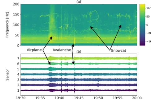
Continuous seismic data were recorded from 12 January to 30 April 2010. These data were previously used by van Herwijnen and Schweizer (2011b), Rubin et al. (2012) and van Herwijnen et al. (2016). The recorded seismic data con-tain various types of events (van Herwijnen and Schweizer, 2011a), including aeroplanes, helicopters and of course avalanches (Fig. 1).
3.1 Pre-processing of the seismic data
While during the 107-day period several hundred avalanches were identified, the vast majority of the data consist of noise or seismic events produced by other sources. To reduce the amount of data to process, we applied a simple
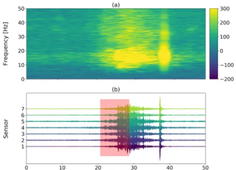
threshold-Figure 1. (a) Spectrogram of an unfiltered 30 min time series.
(b)Corresponding time series. An airplane and an avalanche are visible. Furthermore, noise produced by a snowcat can be seen in the second half of the time series.
Figure 2.Example of the pre-processing:(a)the mean energy val-ues of each window shown as the blue line and the threshold value indicated by the red line;(b) the remaining data cut by the pre-processing step.
based event detection method. It consisted of dividing the continuous seismic data stream in non-overlapping windows of 1024 samples. For each window, a mean absolute ampli-tudeAi was determined. WhenAi≥5A, withA the daily
mean amplitude, the data were used. Furthermore, a data sec-tion of 1t=60 s before and after each event was also in-cluded to ensure that the onset and coda of each event were incorporated. The amount of data to process was thus re-duced by 80 % (Fig. 2).
3.2 Reference avalanche catalogue
Van Herwijnen and Schweizer (2011) visually analyzed the unprocessed seismic time series and the corresponding spec-trogram of one sensor and identifiedN=385 avalanches be-tween 12 January and 30 April 2010. They thus obtained an avalanche catalogue consisting of the release timeti and
du-ration Ti for each avalanche. The onset was defined as the
first appearance of energetic low frequency signals (i.e., be-tween 15 and 25 Hz), while the end of the signal was de-fined as the time when low frequency signals reverted back to background levels. However, only 25 of these avalanches were confirmed by visual observations, i.e., on images ob-tained from automatic cameras. Hence there remains sub-stantial uncertainty about the nature of the identified events.
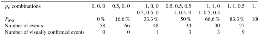
To reduce the uncertainty, three of the authors therefore independently re-evaluated this avalanche catalogue. From the 385 avalanches in the original avalanche catalogue only Npre=283 remained after pre-processing (see Sect. 3.1);
none of the 25 confirmed avalanches were dismissed. By vi-sually inspecting the seismic time series of the seven sen-sors and the stacked spectrogram for each event, they then assigned a subjective probabilitype to each of these
possi-ble avalanche events. Three probabilities were assigned: 1 when it was certain that the observed event was an avalanche, 0 when it was certain that the observed event was not an avalanche and 0.5 when it was uncertain whether the event was an avalanche or not. The probabilities were then com-bined into seven probability classes depending on the mean probability of each event:
Pava=
1 3
3 X
e=1
pe, (1)
with pe the subjective probability that each assigned to a
specific event. In Table 1 the number of events in each probability class is listed. In the reclassified data set, only 20 avalanches were considered as certain avalanche by all three evaluators and 58 events were marked as certainly not an avalanche. Furthermore 18 of the 25 visually confirmed avalanches were within the two highest probability classes.
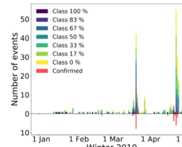
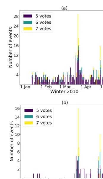
The avalanche activity of the season 2010 is shown in Fig. 3.
Overall, most avalanches were detected in the second half of the investigated period, with two distinct peaks in the avalanche activity around 22 March and 24 April.
The distribution of the event duration changed as the prob-ability class increased (Fig. 4). All events in the lowest proba-bility class had a duration<6 s. More than 90 % of the events had durations≥12 s for the three highest probability classes.
Figure 3.Avalanche activity for the winter season of 2010. The different colors above the zero line indicate the different probability classes derived from the manual detection. The red bars below the zero line indicate the visually confirmed events.
Figure 4.Event duration distribution per probability class.
4 Methods
4.1 Hidden Markov model
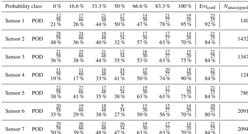
Table 1.Number of events per probability classPavaafter re-evaluation and the corresponding number of confirmed events for each class.
The first row shows the possible combinations of subjective probability (pe): whenpe=1 it was certain that the event was an avalanche;
whenpe=0.5 it was uncertain; and whenpe=0 it was certain that the event was not an avalanche.
pecombinations 0, 0, 0 0.5, 0, 0 1, 0, 0 0.5, 0.5, 0.5 1, 1, 0 1, 1, 0.5 1, 1, 1
0.5, 0.5, 0 1, 0.5, 0 1, 0.5, 0.5
Pava 0 % 16.6 % 33.3 % 50 % 66.6 % 83.3 % 100 %
Number of events 58 66 48 34 30 27 20 Number of visually confirmed events 0 0 1 3 3 9 9
training sets, we used a new approach developed by Hammer et al. (2012). This classification approach exploits the abun-dance of data containing mainly background signals to ob-tain general wave-field properties. Using these properties, a widespread background model can be learned from the gen-eral properties. A new event class is then implemented by using the background model to adjust the event model de-scription by using only one training event. The so-obtained classifier therefore consists of the background model and one model for each implemented event class. The classification process itself calculates the likelihood that an unknown data stream has been generated by a specific class for each indi-vidual class HMM. More detailed information can be found in Hammer et al. (2012); Hammer et al. (2013).
4.2 Feature calculation
Although it is possible to use the raw seismic data as input for the hidden Markov model, we used a compressed form of it, so-called features. Several features can be calculated rep-resenting different aspects of the time series such as spectral, temporal or polarization characteristics. The representation of the seismic signals by features is more adequate to high-light differences between diverse event types. Since we used single component geophones, we only used spectral and tem-poral features. Based on preliminary analysis, we used the following features:
– central frequency – dominant frequency – instantaneous bandwidth – instantaneous frequency – cepstral coefficients – half-octave bands.
A detailed list of the functions used to calculate these features can be found in Hammer et al. (2012).
To calculate the features, we used a sliding window with width,wof 1024 samples. The sliding window is then moved forward with a step of 0.05 s or 25 samples, resulting in an overlap of 97 %.
For the half-octave bands we used a central frequency of fc=1.3 Hz for the first band and a total number of
nine bands. Since the geophones have an eigenfrequency of 14 Hz, only signals with a higher frequency are recorded without any loss of information. However, preliminary re-sults showed that half-octave bands with a central frequency higher thanfmin=5 Hz are adequate.
4.3 Post-processing
The HMM classification resulted in several hundred events in the avalanche class. Many of these events were, however, of very short duration or only identified at one sensor and did not necessarily coincide with avalanches in the reference cat-alogue; i.e., these events were likely false alarms. We there-fore investigated three post-processing methods to reduce the number of false alarms, namely
1. applying a duration threshold for the detected events; 2. analyzing the results of all sensors by introducing a
voting-based classification;
3. analyzing the coherence between all sensors for each detected event.
First, we used an event duration threshold. The duration Tj of any automatically detected eventj was determined by
the HMM. Based on the analysis of van Herwijnen et al. (2013) and van Herwijnen et al. (2016), we can assume that event duration correlates with avalanche size. The first post-processing method therefore consisted of using a minimal durationTminfor the events as described below in Sect. 5.3.1.
Any automatically detected eventj withTj≤Tminwas thus
removed. Similarly, any avalanche i in the reference cata-logue with a durationTi≤Tminwas also removed.
Second, we used a voting-based threshold by tallying the classified events of each sensor. (Rubin et al., 2012) used a similar approach and found that with increasing votes the false alarm rate decreased. The overall idea is that although an avalanche event might not be recorded by one sensor, for instance due to poor coupling of the sensor, it is unlikely that an avalanche is missed by all sensors, especially larger avalanches (Faillettaz et al., 2016). Any automatically de-tected event withVj≤VminwithV the number of votes was
Third, we used a threshold based on the cross-correlation coefficient between the seven sensors. Wave fields gener-ated by avalanches should be relatively coherent, while wave fields generated by noise (e.g., wind) are expected to be incoherent. We therefore divided the seismic data in non-overlapping windows of 1024 samples and for each window we defined a mean normalized correlation coefficient as
R(twin)=
1 Npairs
Npairs X
k=1
rkl(twin), (2)
with Npairs=21 the number of sensor pairs, rkl(twin) the
maximum in the normalized cross correlation between sensor kandlandtwinthe time of the sliding window. The
normal-ized cross correlation is defined as φkl(t )=√ φkl(t )
φkk(0)φll(0)
, (3)
withφkk(0)andφll(0)the zero lag autocorrelation of each
sensor, which is equal to the energy of each single time win-dow. The maximum of the normalized correlation is picked for a maximum lag of tmax=0.05 s, which is the time a
sonic wave field at a speed of 330 m s−1needs to travel the maximum distance between the most distant receiver pair (≈15 m):
rkl(twin)=maxφkl(t ),|t| ≤0.05 s. (4)
The normalized cross correlation only yields values between −1 (perfectly anticorrelated) and 1 (perfectly correlated). A value of 0 means that the signals are completely uncorrelated. Finally, the coherence of each automatically detected event was defined as
Cj=maxR(twin),0≤twin≤Tj. (5)
Any automatically detected event with Cj ≤Cmin was
re-moved.
4.4 Model performance evaluation
To evaluate the performance of the HMM classification, we compared the automatic picks with the reference data set described in Sect. 3.2. To assign an event classified by the HMM as a positive detection we defined a tolerance interval d: the time tjHMM of an event had to be within the interval ti−d≤tjHMM≤ti+d, with ti the release time of the ith
avalanche in the reference data set andd=60 s. The toler-ance intervaldwas necessary, since the release timestiof the
avalanches were picked manually and may contain some un-certainties. In addition, the releases timestjHMM do not nec-essarily coincide with the reference data since the classifier is not an onset picker.
To describe the performance of the classifier we used three values: Nhit,Nunassigned andNmiss. The first valueNhit
de-scribes the total number of avalanches which were correctly
detected by the classifier, i.e., events identified by the classi-fier which corresponded to avalanches in the reference data set. The second value Nunassigned describes the number of
events identified by the classifier which did not correspond to an avalanche in the reference data set. We do not call these events false alarms as during the manual detection some avalanche events might have been missed that are therefore not present in the reference data set. Avalanche events may still be found in the unassigned detections. Finally, the third valueNmissdescribes the number of avalanches in the
refer-ence data that were not identified by the HMM classifier. The three values were used to evaluate the overall model perfor-mance in terms of POD and false alarm ratio (FAR), defined as POD=Nhit/(Nhit+Nmiss)and FAR=Nunassigned/(Nhit+
Nunassigned)(Wilks, 2011).
To determine the best threshold values for the post-processing steps (Sect. 4.3), we plotted POD against FAR values for all probability classes and for different values of Tmin,vminandCmin. One curve therefore illustrates the POD
and FAR with respect to the probability classes for a fixed threshold value. Ideally, when only considering the 100 % probability class, the POD value should be 1 while the FAR value should also be relatively high since all detections of the lower classes are counted as false alarms. By taking more probability classes into account, the FAR will decrease while the POD value should stay close to 1. A perfect model should therefore result in constant POD values of 1 whereas the FAR values should decrease to 0. For realistic models, how-ever, POD and FAR values are expected to decrease when accounting for more probability classes. By plotting POD against FAR values for different threshold values, the opti-mal threshold value can be found by searching for the largest area under the curve (AUC). A perfect model would result in an AUC value of 1, while an AUC value of 0.5 corresponds to a model with a 50–50 chance. Threshold values obtained for models with an AUC value lower than 0.5 are therefore not reliable and any random threshold value can be chosen. In our case, the POD–FAR curves did not span from 0 to 1 on thexaxis. To determine the AUC value we therefore cal-culated the ratio between the area under the POD–FAR curve and the area under the bisector with the samex-axis limits: AUC= AUCHMM
AUCbisector
·0.5. (6)
5 Results
5.1 Temporal feature distribution
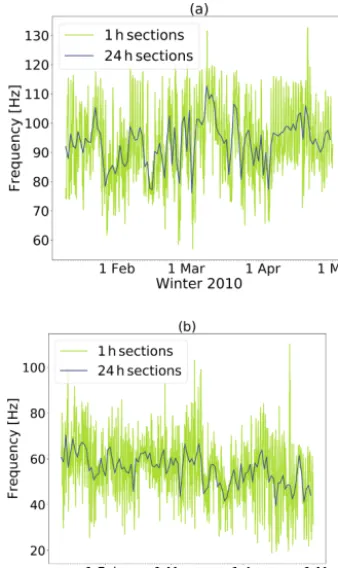
distri-Figure 5. (a)Temporal variations in the central frequency hourly average (yellow) and daily average (blue).(b)Temporal variations in the dominant frequency.
bution at various timescales. First, there were strong diurnal variations (yellow lines in Fig. 5). These were observed in all features (not shown). Second, there were also large variations at longer timescales (blue lines in Fig. 5). While for some features there were significant seasonal trends, for instance for the dominant frequency (Pearsonr= −0.56,p <0.001; Fig. 5b), for others there were no clear trends, for instance for the central frequency (Pearsonr=0.23,p=0.02; Fig. 5a). Building a single background model to classify the entire season would therefore likely not result in a reliable classifi-cation. The background model thus has to be regularly recal-culated. We therefore decided to recalculate the background model each day to classify the events within the same day. 5.2 Training event
While building a representative background model is im-portant, choosing an appropriate training event is of utmost importance for the classifier. As outlined in (van Herwij-nen et al., 2016), the avalanche catalogue consists of var-ious avalanches of different size and type. At the begin-ning of the season the avalanches are most likely dry-snow avalanches, while at the end of the season there a mostly wet-snow avalanches. Our avalanche catalogue only consists of the release time and little information is available on the
Figure 6. (a)Central frequency with normalized time for four dif-ferent avalanche events (colors) from 4 difdif-ferent months. For com-parison, the time was normalized by the event duration, with 0 indi-cating the start of the avalanche and 1 the end of the event.(b) Sec-ond cepstral coefficient.
type of the avalanches. We therefore compared the feature distribution of four different avalanche events, on 21 Jan-uary, 27 FebrJan-uary, 22 March and 24 April 2010, to investigate whether substantial differences related to avalanche type ex-isted (Fig. 6).
While there were some subtle differences in the fea-ture distribution for the four avalanches (e.g., between the avalanches on 21 January and 22 March 2010 in Fig. 6a), overall the four avalanches exhibited very similar behavior. Thus, when viewing avalanches in the feature space, wet- and dry-snow avalanches appear to be very similar. We therefore used one single avalanche class for the HMM classifier and used one training event to learn the model. Specifically, we used an avalanche withPava=100 % recorded on 22 March
2010 (Fig. 7) with a duration of 30 s. However, as seen in Fig. 6, the most rapid changes in feature values occurred at the beginning of the events. In the coda changes in feature values were rather slow, providing limited relevant informa-tion for the classifier. We therefore only used the first 8 s of the training event (marked by the red rectangle in Fig. 7). 5.3 Automatic avalanche classification
5.3.1 Single sensor classification
de-Figure 7.The event used for training the HMM.(a)Stacked spec-trogram of all seven sensors.(b)Seismic waveform for each indi-vidual sensor (colors). The red area highlights the part of the signal used as the training event for the HMM.
Figure 8. (a)POD–FAR curves for sensor 1 for different minimum event durationsTmin(colors).(b)Area under the POD–FAR curve
withTminfor all sensors (colors). The stars show theTminvalue
with the largest area under the curve for each sensor.
tected for each sensor which were not listed in the reference data set. Clearly without any post-processing the number of unassigned events was high.
To reduce the number of unassigned events we applied a minimum duration Tmin to remove events. To obtain a
rea-sonable threshold value, we determined the area under the POD–FAR curve for differentTminvalues (Fig. 8).
Due to the large number of unassigned events (see Table 2) AUC values were generally below 0.5 and using a minimum duration threshold did not result in much improvement. How-ever, for sensors 1 and 6 the number of unassigned events was much lower and there was an optimum Tminthreshold
value around 12 s (Fig. 8 b). In the following, we therefore used the same minimal durationTmin=12 s for all sensors.
While with thisTminthreshold the POD values for the
high-est probability class somewhat decreased, they still remained high (between 68 and 84 %; Table 3). Furthermore, the POD for the confirmed avalanches also remained relatively high,
Figure 9. Classification results using a minimal event duration length of 12 s for(a)sensor 1 and(b)sensor 7. Grey bars show the number of matching detections (hit), blue bars show the unassigned events and the red bars show the events that were not detected as an avalanche (missed). The hatched bars indicate the number of hits (grey) or misses (red) for the confirmed events.
ranging from 60 to 84 %. Note that the duration threshold was also applied to remove events from the reference data set. For a threshold value ofTmin=12 s, the number of events
in the reference data set reduced from 283 to 170 while the number of confirmed avalanches was not affected.
Overall the number of unassigned events substantially de-creased (compare Tables 2 and 3), especially for sensors 1 and 6. For these two sensors the POD values also substan-tially decreased for the lower probability classes but the two main avalanche periods in March and April are clearly visi-ble in the detections (see Fig. 9a for sensor 1). However, for the other sensors, the POD values remained relatively high for the lower probability classes and there were still many unassigned events and the two main avalanche periods were less evident (see Fig. 9b for sensor 7). Clearly, for some of the sensors the number of unassigned events remained very high.
5.3.2 Array-based classification
meth-Table 2.Number of detections (Nhit) and probability of detection (POD) for each sensor and each probability class as well as the POD for
confirmed events Evtconfand number of events that were not in the reference data set (Nunassigned).
Probability class 0 % 16.6 % 33.3 % 50 % 66.6 % 83.3 % 100 % Evtconf Nunassigned
Sensor 1 POD
12 58 17 66 21 48 17 34 14 30 21 27 19 20 23 25 149
21 % 26 % 44 % 50 % 47 % 78 % 95 % 92 %
Sensor 2 POD
28 58 24 66 19 48 11 34 17 30 17 27 14 20 21 25 1432
48 % 36 % 40 % 32 % 57 % 63 % 70 % 84 %
Sensor 3 POD
21 58 25 66 21 48 12 34 16 30 17 27 15 20 21 25 1347
36 % 38 % 44 % 35 % 53 % 63 % 75 % 84 %
Sensor 4 POD
11 58 11 66 16 48 14 34 15 30 20 27 18 20 21 25 124
19 % 17 % 33 % 41 % 50 % 74 % 90 % 84 %
Sensor 5 POD
22 58 27 66 17 48 13 34 19 30 17 27 15 20 21 25 786
38 % 41 % 35 % 38 % 63 % 63 % 75 % 84 %
Sensor 6 POD
20
58 1966 1848 349 1530 1527 1420 2025 2091
35 % 29 % 38 % 27 % 50 % 56 % 70 % 80 %
Sensor 7 POD
29
58 2666 2348 1634 1930 1727 1420 2125 2094
50 % 39 % 48 % 47 % 63 % 63 % 70 % 84 %
Table 3.Number of detections (Nhit) and probability of detection (POD) for each sensor and each probability class as well as the POD
for confirmed events Evtconfand number of events that were not in the reference data set (Nunassigned) using a minimal event duration of Tmin=12 s.
Probability class 0 % 16.6 % 33.3 % 50 % 66.6 % 83.3 % 100 % Evtconf Nunassigned
Sensor 1 POD
0 0 4 39 6 36 11 23 10 26 15 27 16 19 20 25 22
0 % 10 % 17 % 48 % 39 % 56 % 84 % 80 %
Sensor 2 POD
0 0 17 39 12 36 7 23 14 26 17 27 14 19 21 25 408
0 % 44 % 33 % 30 % 54 % 63 % 74 % 84 %
Sensor 3 POD
0 0 14 39 13 36 9 23 13 26 16 27 14 19 20 25 340
0 % 36 % 36 % 39 % 50 % 59 % 74 % 80 %
Sensor 4 POD
0 0 3 38 5 35 6 22 8 26 12 26 15 19 15 25 15
0 % 8 % 14 % 27 % 31 % 46 % 79 % 60 %
Sensor 5 POD
0
0 1639 1136 239 1526 1427 1319 2125 157
0 % 41 % 31 % 39 % 58 % 52 % 68 % 84 %
Sensor 6 POD
0
0 397 1336 235 1026 1427 1319 1825 597
0 % 18 % 36 % 22 % 39 % 52 % 69 % 72 %
Sensor 7 POD
0 0 17 39 14 36 10 23 15 26 17 27 14 19 21 25 653
0 % 43 % 39 % 44 % 58 % 63 % 74 % 84 %
ods the detections from all sensors were pooled, the number of unassigned events was very high. This resulted in much higher FAR values and thus poor model performance with low AUC values, all below 0.5. Arbitrary values forvminor
Cmin could therefore be chosen. However, the overall goal
of these post-processing steps was to reduce the number of unassigned events, while still retaining a reasonable POD.
We therefore analyzed the effect of different threshold values on FAR values as well as on POD values for the probability classes.
unas-Figure 10. (a) POD for each probability class depending on the minimum number of votes (colors). (b) Number of unassigned events for different number of votes (colors).
Figure 11. (a) POD for each probability class depending on the minimal coherence (colors).(b)Number of unassigned events for different coherence threshold values (colors).
signed events. Following the same procedure we selected a coherence value of 0.6. Using this value, the POD was rel-atively high and the number of unassigned events could be reduced to less than 100 events.
In total, we thus have three different post-processing steps which can be applied to the data: a minimal event dura-tion Tmin=12 s, a minimum number of votesvmin=5 and
a coherence thresholdCmin=0.6. By combining these three
steps, six array-based post-processing workflows were im-plemented:
– v:vj≥vmin
– c:Cj ≥Cmin
– vc:vj≥vminandCj≥Cmin
– t v:Tj≥Tminandvj≥vmin
– t c:Tj≥TminandCj≥Cmin
– t vc:Tj≥Tmin,vj≥vminandCj ≥Cmin.
The number of unassigned events decreased most with a combined approach always including the number of votes (vc,t v, ort vcin Fig. 12). When using only one array-based
Figure 12. (a)POD for each probability class for different post-processing workflows (colors).vis minimal number of votes used,
tis minimal event duration andcis minimal coherence.(b)Number of unassigned events remaining after the post-processing for each workflow.
Figure 13.All events detected by at least five sensors. The different colors indicate the number of votes.(a)The results without any lim-itation of the duration of the events are plotted.(b)Only events with a minimum duration as mentioned before are taken into account. On the right the two main avalanche periods are more clearly visible.
probability classes were obtained for the voting-based pro-cessing with and without a minimal duration of the events (vandt vin Fig. 12a). For both these post-processing work-flows the two periods of high avalanche activity are visible (Fig. 13). However, by also applying the duration threshold, the total number of detections decreased and the two periods in March and April became more clearly visible (Fig. 13b). 5.3.3 Unassigned events
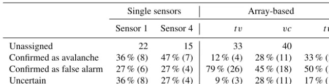
We compared the automatic detections with the reference avalanche catalogue and obtained a large number of unas-signed events. It remains unclear whether the unasunas-signed events are all false alarms or partly correspond to avalanches that were not identified in the reference data. We therefore visually inspected the unassigned events. In order to keep this reanalysis manageable, we only focused on the post-processing steps which resulted in less than 50 unassigned events. Thus, we individually investigated single sensor re-sults from sensor 1 and 4 withTmin=12 s and array-based
results fort v,vcandt vc. The visual inspection showed that for the single sensor results between 36 and 47 % of the unas-signed events were likely unidentified avalanches and less than one-third were false alarms (Table 4). For the array-based results, however, most of the unassigned events (be-tween 45 and 79 %) were false alarms while fewer events were likely associated with avalanches that were missed by van Herwijnen and Schweizer (2011a).
6 Discussion and summary
We trained HMMs, a machine learning algorithm, to au-tomatically detect avalanches in continuous seismic data recorded near an avalanche starting zone above Davos, Switzerland, for the winter season of 2010. To reduce the amount of data to process, we pre-processed the continuous data using an amplitude threshold (Fig. 2). We then imple-mented single sensor and array-based post-processing steps and the performance of the models was evaluated using a previously published reference avalanche catalogue obtained from the same seismic data (van Herwijnen and Schweizer, 2011a; van Herwijnen et al., 2016).
After pre-processing the data, the reference avalanche cat-alogue contained 283 avalanches between 12 January and 30 April 2010, events that were identified by visual inspection of the waveform and spectrogram of a single sensor (van Her-wijnen and Schweizer, 2011a). Since only 25 of these events were independently confirmed avalanches, considerable un-certainty remained about the identified events. To reduce the uncertainty in the reference catalogue, three of the authors therefore re-evaluated the data. This allowed us to assign seven subjective probability classes between 0 and 100 % to each event. Overall, only 20 events were marked as certain avalanche (Table 1) and hence the performance of the
clas-sifiers can only be evaluated for these particular events. For the remaining events, there are still uncertainties and hence the performance of the classifier can only be estimated. Fur-thermore, this reanalysis highlighted the difficulty in obtain-ing an objective and reliable reference avalanche catalogue. It also showed that expert decisions are biased and there is a need for a reliable automatic classifier to identify avalanches in continuous seismic data.
Recent work by Hammer et al. (2017) showed very promising results for applying a HMM to automatically de-tect avalanches in continuous seismic data. While they only focused on a 5-day period during an exceptional avalanche cycle in 1999, our goal was to classify continuous seismic data spanning more than 100 days. This prevented us from building a single background model to classify the entire sea-son since temporal variations in feature distributions at var-ious timescales were present (Fig. 5). Indeed, when using a single background model to classify the entire season for sen-sor 1 only two-thirds of the events were detected by having almost 6 times the number of unassigned events. One pos-sible reason for these variations in feature distribution was likely the setup of the sensor array. The geophones were packed in a Styrofoam housing and inserted within the snow-pack. As such, less snow covered the sensors than if they had been inserted in the ground, making them more suscepti-ble to environmental noise. Furthermore, it is also likely that the snow cover introduced additional noise in spring due to the rapid settlement and water infiltration. We therefore re-calculated the background model for each day and for each sensor to classify the data from the same day. However, for the operational implementation this would be impractical, since there would always be a 24 h delay in the detections. Other strategies for regularly updating the background model should therefore be investigated (e.g., Riggelsen and Ohrn-berger, 2014).
Table 4.Results of the reanalysis of the detections not covered by the test data set. Left side of the table shows the results of the reanalysis of two single sensors, while the right side shows the results of the array-based classification. For the single sensors a minimum duration for the events oftmin=12 s was taken into account. The voting-based processing steps analyzed are minimum number of votes (v), minimum
duration (t) and coherence (c).
Single sensors Array-based
Sensor 1 Sensor 4 t v vc t vc
Unassigned 22 15 33 40 6
Confirmed as avalanche 36 % (8) 47 % (7) 12 % (4) 28 % (11) 33 % (2) Confirmed as false alarm 27 % (6) 27 % (4) 79 % (26) 45 % (18) 50 % (3) Uncertain 36 % (8) 27 % (4) 9 % (3) 28 % (11) 17 % (1)
the slope closest to a cornice where the snow was the deepest (van Herwijnen and Schweizer, 2011a). The other five sen-sors were covered by less snow due to local inhomogeneities, leaving these sensors more sensitive to environmental noise. For future deployments it will thus be important to deploy the sensors below a homogeneous snow cover and not within the snow cover. This should reduce the amount of environmental noise and consequently the number of false alarms.
To further reduce the number of false alarms, we im-plemented two array-based post-processing steps, namely a voting-based approach and a signal coherence threshold. In combination with the minimal event duration, we thus inves-tigated six array-based post-processing workflows. Results showed that these array-based methods were effective in re-ducing the number of unassigned events (Fig. 12). However, the POD values generally also decreased, resulting in overall fewer detections. Combined post-processing methods which included the voting-based approach resulted in better model performance, in line with results presented by Rubin et al. (2012). The best model performance was obtained by com-bining the event duration threshold for events with at least five votes. The number of unassigned events reduced to about 30 and POD values were highest (∼55 %) for the highest probability class and decreased for the lower classes. De-spite the large differences in model performance for the in-dividual sensors, the model still performed marginally better when pooling the data from the entire array. These results are promising as with an improved sensor deployment strategy array-based post-processing is likely to further improve.
Comparing our model performance to previously pub-lished studies is not straightforward. We assigned subjec-tive probability classes to our reference avalanche catalogue rather than using a yes or no approach. Furthermore, we used geophones deployed in an avalanche starting zone, while Bessason et al. (2007), Leprettre et al. (1996) and Ham-mer et al. (2017) used sensitive broadband seismometers de-ployed at valley bottom. Therefore, it is very likely that there was more environmental noise in our data and many of the detected avalanches in our reference data set were rather small (van Herwijnen et al., 2016). Given these differences in instrumentation and deployment, our detection results are
encouraging and highlight the advantage of using HMMs for the automatic identification of avalanches in continuous seis-mic data.
The main advantages of the proposed approach is that only one training event (Fig. 7) is needed to classify the entire sea-son. As shown by Hammer et al. (2017), for large avalanches it is possible to build a HMM with a high POD and very low FAR with one training event. Even though we used less-sensitive sensors in this work, we were also able to iden-tify periods of high avalanche activity (compare Fig. 3 with Figs. 9 and 13). Furthermore, when only considering the vi-sually confirmed avalanches, the POD was typically around 80 % (see Tables 2 and 3). This suggests that HMMs can eas-ily be implemented at new sites. In contrast, the model used by Bessason et al. (2007) relied on a 10-year database, and Leprettre et al. (1996) used a set of fuzzy logic rules derived by the experts. Note that the post-processing steps we inves-tigated are likely site dependent, in particular the event dura-tion threshold. However, such a threshold value is intuitive, has a linear influence on model outcome and is thus easily tunable.
For operational use, the model should be able to automat-ically detect avalanches in near real time. The main disad-vantage of the proposed approach is its computational cost. The feature calculation for 1 day takes≈1 h for the pre-processed data and≈7 h for the unprocessed data. Replac-ing the used features with computationally less expensive at-tributes would decrease the processing time drastically and encourage real-time applications.
In this work, we classified the data from each sensor in-dividually, requiring a separate background model for each sensor. The results from the different sensors were then combined using post-processing rules either on a voting-based approach or taking the coherence into account. Strictly speaking, the coherence could have been added to the model as an additional feature. However, calculating the coher-ence for 21 receiver pairs, even after applying the amplitude threshold during pre-processing, was still very time consum-ing (≈200 % real time).
seis-mic data. The variable model performance between the dif-ferent sensors highlighted problems which can likely be over-come by improving the sensor deployment strategy. Specif-ically, we suggest that the sensors should be deployed 30 to 50 cm underground at a site with a homogeneous and preferably thick snow cover and to increase the distance be-tween the sensors to apply array processing techniques for source localization (Lacroix et al., 2012). In addition, further avalanche events may be used for training to improve model performance. Finally, incorporating localization parameters as new features in the HMM could open the door for further model improvement, as is done for the automatic detection of avalanches in continuous infrasound data (Marchetti et al., 2015; Thüring et al., 2015). These features can then either be implemented directly into the HMM or be used in additional post-processing steps.
Data availability. Due to the huge amount of seismic raw data and parameterized waveforms, we are not able to provide these data. Instead we provide a data package containing the classification re-sults, the reference data set, the start and end times of the pre-processed seismic data and some Python scripts. The data are avail-able under the following: https://doi.org/10.16904/envidat.29 (Heck and van Herwijnen, 2018).
Competing interests. The authors declare that they have no conflict of interest.
Acknowledgements. Matthias Heck was supported by a grant of the Swiss National Science Foundation (200021_149329). We thank numerous colleagues from SLF for help with field work and maintaining the instrumentation.
Edited by: Margreth Keiler
Reviewed by: Naomi Vouillamoz and one anonymous referee
References
Bessason, B., Eiriksson, G., Thorarinsson, O., Thorarinsson, A., and Einarsson, S.: Automatic detection of avalanches and debris flows by seismic methods, J. Glaciol., 53, 461–472, 2007. Beyreuther, M., Hammer, C., Wassermann, J., and Ohrnberger, M.:
Constructing a Hidden Markov Model based earthquake detec-tor: application to induced seismicity, Geophys. J. Int., 189, 602– 610, 2012.
Caplan-Auerbach, J. and Huggel, C.: Precursory seismic-ity associated with frequent, large ice avalanches on Il-iamna volcano, Alaska, USA, J. Glaciol., 53, 128–140, https://doi.org/10.3189/172756507781833866, 2007.
Dammeier, F., Moore, J. R., Hammer, C., Haslinger, F., and Loew, S.: Automatic detection of alpine rockslides in continuous seis-mic data using hidden Markov models, J. Geophys. Res.-Earth, 121, 351–371, 2016.
Faillettaz, J., Funk, M., and Vincent, C.: Avalanching glacier instabilities: Review on processes and early warning perspectives, Rev. Geophys., 53, 203–224, https://doi.org/10.1002/2014RG000466, 2015.
Faillettaz, J., Or, D., and Reiweger, I.: Codetection of acoustic emis-sions during failure of heterogeneous media: New perspectives for natural hazard early warning, Rev. Geophys., 43, 1075–1083, https://doi.org/10.1002/2015GL067435, 2016.
Hammer, C., Beyreuther, M., and Ohrnberger, M.: A seismic-event spotting system for Volcano fast-response systems, B. Seismol. Soc. Am., 102, 948–960, 2012.
Hammer, C., Ohrnberger, M., and Fäh, D.: Classifying seismic waveforms from scratch: a case study in the alpine environment, Geophys. J. Int., 192, 425–439, 2013.
Hammer, C., Fäh, D., and Ohrnberger, M.: Automatic detection of wet-snow avalanche seismic signals, Nat. Hazards, 86, 601–618, https://doi.org/10.1007/s11069-016-2707-0, 2017.
Harrison, J.: Seismic signals from avalanches, Armstrong and Ives (Eds.), Avalanche release and snow characteristics. Institute of Arctic and Alpine Research, University of Colorado, Occasional Paper No. 19, 145–150, 1976.
Heck, M. and van Herwijnen, A.: Automatic detection of avalanches; WSL Institute for Snow and Avalanche Research SLF, https://doi.org/10.16904/envidat.29, 2018.
Kishimura, K. and Izumi, K.: Seismic signals induced by snow avalanche flow, Nat. Hazards, 15, 89–100, 1997.
Lacroix, P., Grasso, J.-R., Roulle, J., Giraud, G., Goetz, D., Morin, S., and Helmstetter, A.: Monitoring of snow avalanches using a seismic array: Location, speed estimation, and relationships to meteorological variables, J. Geophys. Res.-Earth, 117, F01034, https://doi.org/10.1029/2011JF002106, 2012.
Leprettre, B., Navarre, J., and Taillefer, A.: First results from a pre-operational system for automatic detection and recognition of seismic signals associated with avalanches, J. Glaciol., 42, 352– 363, 1996.
Leprettre, B., Martin, N., Glangeaud, F., and Navarre, J.: Three-Component Signal Recognition Using Time, Time–Frequency, and Polarization Information – Application to Seismic Detection of Avalanches, IEEE T. Signal Process., 46, 83–102, 1998. Marchetti, E., Ripepe, M., Ulivieri, G., and Kogelnig, A.:
Infra-sound array criteria for automatic detection and front velocity es-timation of snow avalanches: towards a real-time early-warning system, Nat. Hazards, 15, 2545–2555, 2015.
Ohrnberger, M.: Continuous automatic classification of seismic sig-nals of volcanic origin at Mt. Merapi, Java, Indonesia, PhD the-sis, 19–58, 71–112, 2001.
Pérez-Guillén, C., Sovilla, B., E. Suriñach, E., Tapia, M., and Köh-ler, A.: Deducing avalanche size and flow regimes from seismic measurements, Cold Reg. Sci. Tech., 121, 25–41, 2016. Podolskiy, E. A. and Walter, F.: Cryoseismology, Rev. Geophys.,
54, 708–758, https://doi.org/10.1002/2016RG000526, 2016. Rabiner, L.: A tutorial on Hidden Markov Models and selected
ap-plication in speech recognition, P. IEEE, 77, 257–286, 1989. Riggelsen, C. and Ohrnberger, M.: A Machine Learning
Ap-proach for Improving the Detection Capabilities at 3C Seismic Stations, Pure Appl. Geophys., 171, 395–411, https://doi.org/10.1007/s00024-012-0592-3, 2014.
IEEE International Conference on Machine Learning and Appli-cations, 1, 13–20, 2012.
Sabot, F., Naaim, M., Granada, F., Suriñach, E., Planet, P., and Furada, G.: Study of avalanche dynamics by seismic meth-ods, image-processing techniques and numerical models, Ann. Glaciol., 26, 319–323, 1998.
Schaerer, P. A. and Salway, A. A.: Seismic and impact-pressure monitoring of flowing avalanches, J. Glaciol., 26, 179–187, 1980. St. Lawrence, W. and Williams, T.: Seismic signals associated with
avalanches, J. Glaciol., 17, 521–526, 1976.
Suriñach, E., Sabot, F., Furdada, G., and Vilaplana, J.: Study of seis-mic signals of artificially released snow avalanches for monitor-ing purposes, Phys. Chem. Earth Pt. B, 25, 721–727, 2000. Suriñach, E., Furdada, G., Sabot, F., Biescas, B., and Vilaplana,
J.: On the characterization of seismic signals generated by snow avalanches for monitoring purposes, Ann. Glaciol., 32, 268–274, https://doi.org/10.3189/172756401781819634, 2001.
Suriñach, E., Vilajosana, I., Khazaradze, G., Biescas, B., Fur-dada, G., and Vilaplana, J. M.: Seismic detection and charac-terization of landslides and other mass movements, Nat. Haz-ards Earth Syst. Sci., 5, 791–798, https://doi.org/10.5194/nhess-5-791-2005, 2005.
Thüring, T., Schoch, M., van Herwijnen, A., and Schweizer, J.: Ro-bust snow avalanche detection using supervised machine learn-ing with infrasonic sensor arrays, Cold Reg. Sci. Technol., 111, 60–66, 2015.
van Herwijnen, A. and Schweizer, J.: Seismic sensor array for mon-itoring an avalanche start zone: design, deployment and prelimi-nary results, J. Glaciol., 57, 257–264, 2011a.
van Herwijnen, A. and Schweizer, J.: Monitoring avalanche activity using a seismic sensor, Cold Reg. Sci. Technol., 69, 165–176, 2011b.
van Herwijnen, A., Dreier, L., and Bartelt, P.: Towards a basic avalanche characterization based on the generated seismic signal, Proceedings 2013 International Snow Science Workshop, Greno-ble, France, 1033–1037, 2013.
van Herwijnen, A., Heck, M., and Schweizer, J.: Forecasting snow avalanches by using highly resolved avalanche activity data ob-tained through seismic monitoring, Cold Reg. Sci. Technol., 132, 68–80, 2016.
Vilajosana, I., Khazaradze, G., Surinach, E., Lied, E., and Kristensen, K.: Snow avalanche speed determination us-ing seismic methods, Cold Reg. Sci. Technol., 49, 2–10, https://doi.org/10.1016/j.coldregions.2006.09.007, 2007a. Vilajosana, I., Suriñach, E., Khazaradze, G., and Gauer,
P.: Snow avalanche energy estimation from seismic signal analysis, Cold Reg. Sci. Technol., 50, 72–85, https://doi.org/10.1016/j.coldregions.2007.03.007, 2007b. Wilks, D. S.: Statistical methods in the atmospheric sciences, Vol.
100, Academic press, 2011.