i
EFFECT OF INCLINED MAGNETIC FIELD IN MHD FLOWS PAST A VERTICAL PLAT IN PRESENCES OF HALL CURRENT
A DISSERTATION SUBMITTED IN PARTIAL FULFILLMENT OF THE REQUIREMENT FOR THE DEGREE OF MASTER OF SCIENCE AND APPLIED MATHEMATICS IN THE SCHOOL OF PURE AND APPLIED SCIENCES OF KENYATTA UNIVERSITY
JULY, 2019 BY
ZEINAB ALI MOHAMED 156/CE/26265/2014
ii
DECLARATION
I Zeinab Ali Mohamed, hereby declare that the contents of this dissertation represent my own work and that this dissertation has not been previously submitted for any academic examination towards any degree or masters qualification at any other university.
Furthermore, it represents my own opinions and not necessarily those of Kenyatta University.
Signature: ... Date...
Zeinab Ali Mohamed
I confirm that the work reported in this dissertation was carried out by the candidate
Under my supervision.
Signature: ... Date...
iii
DEDICATIONiv
ACKNOWLEDGEMENTS
First, I would like to thank my project supervisor; Dr. Amos Magua, who dedicated his time and took the responsibility of guiding me throughout the project work. The discussions and encouragement always revitalized my hopes and rekindled the desire to continue.
My humble gratitude and appreciation go to the staff of Kenyatta University in the School of Pure and Applied Science particularly academic staff of the department of mathematics for having given me the much needed opportunity and to use the excellent facilities. Thank you all for your support and encouragement I received.
I also wish to appreciate my course mates, colleagues who encouraged me always. A quick mention of some of them like Alex and Nzioka is in order. The time I spent with you is always special and memorable. You expanded my horizon during our interaction.
I cannot forget my family who had to content with my seemingly perennial failures from time to time as I was pursuing this work. Thank you, may the Good Lord bless you all.
v
ABSTRACTvi
NOMENCLATURE
SYMBOL QUANTITY UNIT
B Magnetic induction vector
p
C Specific heat, J KgK
D Diffusion coefficient 2
/
m s
g
F Body force, N
e
F Electromagnetic force, N
g Acceleration due to gravity 2
m s
Gr Grashof number
h Specific enthalpy K Kg
0
H Magnitude of the magnetic field
J Current density A m2
z y
x J J
J , , Components of current density, 2
A m
k Thermal conductivity w mk
M Magnetic field parameter
Pr Prandtl number
q Velocity of the fluid m s
Q Heat flux vector 2
W m
Sc Schmidt number
w
T Dimensional temperature of the fluid at the plate K
T Dimensionless temperature of the fluid K
Coefficient of volumetric expansion 1 K
e
Electron cyclotron frequency HzE Electric field volts m
e Electric charge 3
/m coul
e
Collision time of electrons s0
L Hall current parameter
Dimensionless temperature of fluid
Fluid density 3Kg m
v Kinematics viscosity of the fluid 2
m s
Dynamic viscosity of the fluid, 1Kgm s
Electrical conductivity 1m
t
Dimensionless timet
Time interval
x
y z Distance intervals
U Free stream velocity m s
w v
u , , Velocity components, m s
z y
viii
TABLE OF CONTENTS
DECLARATION ... ii
DEDICATION ... iii
ACKNOWLEDGEMENTS... iv
ABSTRACT ... v
NOMENCLATURE ... vi
TABLE OF CONTENTS ... viii
CHAPTER ONE ... 1
1.0 Introduction ... 1
1.1 Background ... 1
1.2 Definition of terms ... 2
1.2.1 Forward finite and central finite difference formulae ... 3
1.2.2 Mass diffusion ... 4
1.2.3 Angle of inclination ... 5
1.2.4 Magnetic field ... 5
1.2.5 Schmidt number ... 6
1.2.6 Hall parameter ... 6
1.2.7 Definition of mesh ... 7
1.3 PROBLEM STATEMENT AND JUSTIFICATION ... 8
I.4 OBJECTIVES ... 9
1.4.1 GENERAL RESEARCH OBJECTIVES ... 9
1.4.2 SPECIFIC RESEARCH OBJECTIVES ... 9
1.5 SIGNIFICANCE OF THE STUDY ... 9
1.6 APPLICATIONS ... 10
1.6.1 Geophysics ... 10
1.6.2 Earthquakes ... 10
1.6.3 Astrophysics ... 10
1.6.4 Sensors ... 10
1.6.5 Engineering ... 11
CHAPTER TWO ... 12
2.0 LITERATURE REVIEW ... 12
CHAPTER THREE ... 14
ix
3.1 MODEL ASSUMPTIONS ... 14
3.2 MODEL EQUATIONS ... 14
3.2.1 GENERAL EQUATIONS GOVERNING THE FLUID FLOW ... 14
3.2.2 CONTINUITY EQUATION ... 14
3.2.3 NAVIER-STOKES’S EQUATION ... 15
3.2.4 ENERGY EQUATION ... 16
3.2.5 THE CONCENTRATION EQUATION. ... 18
3.2.6 MAXWELL’S EQUATIONS ... 19
3.2.7 OHM’S LAW ... 19
3.2.7 CONSERVATION OF ELECTRIC CHARGE ... 19
3.4 SPECIFIC GOVERNING EQUATIONS. ... 20
3.4.1 CONTINUITY EQUATION ... 21
3.4.2 MOMENTUM EQUATION ... 22
3.4.3 ENERGY EQUATION ... 26
3.4.4 CONCENTRATION EQUATION ... 27
3.5 APPROXIMATIONS AND ASSUMPTIONS ... 28
CHAPTER FOUR ... 30
4.0 RESULT FINDINGS ... 30
4.1 NUMERICAL METHOD OF SOLUTION ... 30
4.3 NON-DIMENSIONALISATION ... 31
THE NUMERICAL SOLUTION ... 34
CHAPTER FIVE ... 36
5.0 recommendation and summary... 36
5.2 Observations ... 49
5.3 Conclusion ... 49
5.4 RECOMENDATION ... 49
1
CHAPTER ONE
1.0 Introduction
In this chapter, the main terminologies used are introduced and defined for the study of the effect of inclination of the magnetic field with variable temperature and mass diffusion in MHD flow past a vertical plate in the presence of hall current in details. The statement of the problem, objectives of the study and the significance are also discussed
1.1 Background
An unsteady viscous incompressible electrically conducting fluid past an impulsively started oscillating vertical plane whereby the magnetic field is applied at an angle α is considered here. The plate is electrically conducting. A uniform magnetic field, Bo is applied at an angle of inclination α to the flow .At a time 𝑡 = 0 the temperature of the fluid and the plate is T∞ and concentration of the fluid is C∞. .At time 𝑡 > 0, the plate starts oscillating in its own plane with frequency w, the concentration of the fluid and the temperature of the plate are raised to Cw and Tw. 𝑇ℎ𝑒 the magnetic field is given by
𝐵0 = 𝐵0𝑥𝑖 + 𝐵0𝑦𝑗 + 𝑂𝐾
Where𝐵0𝑥 = |𝐵⃗⃗⃗⃗ |𝑐𝑜𝑠𝛼 = 𝐵0 0cos 𝛼
𝐵0𝑦 = |𝐵⃗⃗⃗⃗ | sin 𝛼 = 𝐵0 0sin 𝛼 𝐵0 = 𝐵0cos 𝛼 𝑖 + 𝐵0sin 𝛼 𝑖 + 𝑂𝐾
= (𝐵0cos 𝛼 , 𝐵0sin 𝛼 , 0)
2
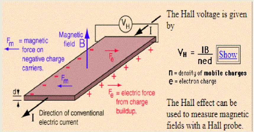
1.2 Definition of termsMHD- MHD is the study of the dynamics of electrically conducting fluids. Such fluids include: Liquid metals (Mercury, Gallium, and Molten Iron), salt water or electrolytes, plasmas. MHD is comprised of three words. Magneto meaning magnetic, hydro meaning fluids and dynamics meaning movement. MHD was initiated by Hannes Alfven (2012). The concept behind MHD is that magnetic fields can induce currents in a moving conductive fluid which in turn creates forces on the fluid and also changes the magnetic field itself. The set of equations which describe MHD are a combination of the Navier-Stokes equations of fluid dynamics and Maxwell‟s equations of electromagnetism.
3
Figure 1: Hall Effect1.2.1 Forward finite and central finite difference formulae METHOD OF SOLUTION
The above system of equations together with the initial and boundary conditions are solved numerically by finite difference method. To relate the partial derivatives in the differential equations to the function values at the adjacent nodal points, a uniform mesh is used. We divide the x-z plane into a network of uniform rectangular cells of height ∆x and width ∆zas shown in figure 2, where i and k refer to x and z respectively. If ∆x represents an increment in x and represents an increment in z, then x= i∆x and z = k∆z
The finite difference approximations of the partial derivatives in equations ++are obtained using Taylor series expansion of the dependent variable about the grid point (k, i)
𝜙(𝑘 − 1, 𝑖) = 𝜙(𝑘 − 𝑖) − 𝜙′(𝑘 − 𝑖)Δ𝑧 +1 2𝜙
′(𝑘, 𝑖)(Δ𝑧)2−1 6𝜙
"(𝑘 − 𝑖)(Δ𝑧)3….. (2.21)
𝜙(𝑘 + 1, 𝑖) = 𝜙(𝑘, 𝑖) + 𝜙′(𝑘, 𝑖)Δ𝑧 +1 2𝜙
′(𝑘, 𝑖)(Δ𝑧)2+1 6𝜙
"(𝑘, 𝑖)(Δ𝑧)3+…. (2.22)
4
𝜙′ = 𝜙(𝑘+1,𝑖)−𝜙(𝑘−1,𝑖)2Δ𝑧 …….. (2.23)
On eliminating from equations (2.22) and (2.23), we have
𝜙" =𝜙(𝑘+1,𝑖)−2𝜙(𝑘,𝑖)+𝜙(𝑘−1,𝑖)
(Δ𝑥)2 …….. (2.24)
Central difference formulas for the first and second derivatives with respect to x are: 𝜙′ = 𝜙(𝑘+1,𝑖)−𝜙(𝑘−1,𝑖)
2Δ𝑥 ……… (2.25) 𝜙" =𝜙(𝑘+1,𝑖)−2𝜙(𝑘,𝑖)+𝜙(𝑘−1,𝑖)
(Δ𝑥)2 ………….. (2.26)
In forward difference, we have
𝜙′ = 𝜙(𝑘+1,𝑖)−𝜙(𝑘,𝑖)
Δ𝑧 ……… (2.27) 𝜙" =𝜙(𝑘+1,𝑖)−2𝜙(𝑘,𝑖)+𝜙(𝑘−1,𝑖)
(Δ𝑧)2 ………….. (2.28)
𝜙′ = 𝜙(𝑘+1,𝑖)−𝜙(𝑘,𝑖)
Δ𝑥 ……… (2.29)
In this research, we use the subscripts to indicate spatial points and superscripts to indicate time 𝑇𝑘,𝑖𝑛+1 = (𝑧𝑘, 𝑥𝑖, 𝑡𝑛+1) If we let the mesh point variable at time tn to be denoted by 𝜙(𝑘,𝑖)𝑛 , the forward difference for the first order derivatives with respect to time t is given by:
𝜙(𝑘,𝑖)𝑛 = 𝜙(𝑘,𝑖)
𝑛+1−𝜙 (𝑘,𝑖) 𝑛
Δ𝑡 …… (2.30) 1.2.2 Mass diffusion
Mass transfer happens due to relative activity of each molecule.
5
Figure 2: Mass Diffusion1.2.3 Angle of inclination
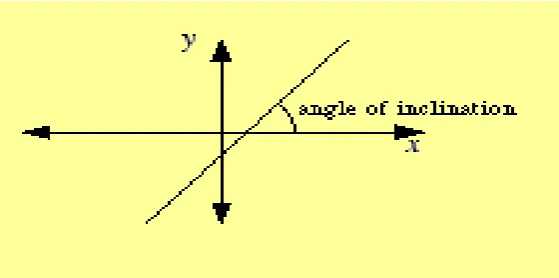
The angle between a line and the x-axis. This angle is between 0 and 90 and is measured counterclockwise from the part of the x-axis to the right of the line.
Figure 3: Angle of inclination
1.2.4 Magnetic field
6
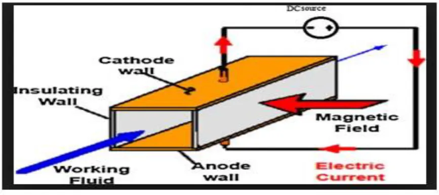
Figure 4: Magnetic Field1.2.5 Schmidt number
Schmidt Number, Sc, is a dimensionless parameter representing the ratio of diffusion of momentum to the diffusion of mass in a fluid. It is defined as 𝑆𝑐 = 𝑣 𝛿⁄ where ν is kinematic viscosity and δ diffusivity.
1.2.6 Hall parameter
The Hall Parameter, β, in plasma can take values between 1 and 5. The following formula is
used:
where: 𝛽 = 𝑒𝐵 𝑀𝑒𝑉
e = elementary charge
B = magnetic field
Me = electron mass
7
1.2.7 Definition of meshIn order to give a relation between the partial derivatives in the differential equation and the function values at the adjacent nodal points, we use a uniform mesh. Let the x-y plane be divided into a network of uniform rectangular cells of width y and heightx, as shown below.
Let m and n refer to x and y respectively
If we let y represent increment in y and x represent increment in x then y= my and
x = n .The finite difference approximations of the partial derivatives are obtained by Taylor series expansion of the dependent variable.
' 1 '' 2 1 ''' 3
( 1, ) ( , ) ( , ) ( , )( ) ( , )( ) ...4.1
2 6
m n m n m n y m n y m n y
𝜓(𝑚 + 1, 𝑛) = 𝜓(𝑚, 𝑛) + 𝜓(𝑚, 𝑛)∆𝑦 +1 2𝜓
0(𝑚. 𝑛)(Δ𝑦)2+1 6𝜓
0(𝑚. 𝑛)(Δ𝑦)3+……...2.5
On eliminating
''from equation (4.1) and (4.2) yieldsx
8
' ( 1, ) ( 1, )
2
m n m n
Hot y
……….………2.6
On eliminating
'from equation (4.1) and (4.2) results to''
2
( 1, ) 2 ( , ) ( , ) ( )
m n m n m n
Hot y
……….2.7
Similarly
' ( , 1) ( , 1)
2
m n m n
Hot x ……….2.8 '' 2
( , 1) 2 ( , ) ( , 1) ( )
m n m n m n
Hot x
………..2.9
1.3 PROBLEM STATEMENT AND JUSTIFICATION
9
I.4 OBJECTIVES1.4.1 GENERAL RESEARCH OBJECTIVES
To study the effect of inclination of the magnetic field with variable temperature and mass diffusion in MHD flow past a vertical plate in the presence of hall current.
1.4.2 SPECIFIC RESEARCH OBJECTIVES
1. To develop the equation governing MHD fluid flow with inclined magnetic field.
2. To determine the effects of varying the angle of magnetic inclination on velocity,
temperature and concentration.
3. To determine the effects of varying the flow parameters i.e Gr, Pr, Sc and Gm on the
flow variables when the applied magnetic field is inclined.
1.5 SIGNIFICANCE OF THE STUDY
10
applications; devices based on this relatively simple relationship between current, magnetic field and voltage can be used to measure position, speed and magnetic field strength.
1.6 APPLICATIONS
1.6.1 Geophysics
Beneath the Earth's mantle lies the core, which is made up of two parts: the solid inner core and liquid outer core. Both have significant quantities of iron. The liquid outer core moves in the presence of the magnetic field and eddies are set up into the same due to the Coriolis effect.
1.6.2 Earthquakes
Some monitoring stations have reported that earthquakes are sometimes preceded by a spike in ultra-low frequency (ULF) activity.
1.6.3 Astrophysics
MHD applies to astrophysics, including stars, the interplanetary medium (space between the planets), and possibly within the interstellar medium (space between the stars) and jets.
1.6.4 Sensors
Principle of MHD sensor for angular velocity measurement
11
1.6.5 EngineeringMHD is related to engineering problems such as plasma confinement, liquid-metal cooling of nuclear reactors, and electromagnetic casting (among others).
12
CHAPTER TWO
2.0 LITERATURE REVIEW
Magneto hydrodynamics (MHD) flow with heat transfer is one of the classes of flow in fluid mechanics which has received considerable attention in recent decades. This is due to the advancement of numerous transport processes in engineering and industries where the flow is applied. Some of the areas where this type of flow is applied are in the extrusion of polymer in the melt spinning process, dispersion of metals, metallurgy, design of MHD pumps and MHD generators. The performances presented by Nano fluids have led to innovative way of improving the thermophysical properties of working fluids. Choi (1995) experimentally demonstrated the anomalous convective heat transfer enhancement when nanometer-sized particles are suspended in the base fluid. These tiny particles are made up of materials that are chemically stable.
13
14
CHAPTER THREE
3.0 METHODOLOGY
3.1 MODEL ASSUMPTIONS
The model assumptions made are as follows; - The flow is steady and lamina.
- The fluid is viscous and incompressible. - The fluid is electrically conducting. - The plate is electrically non-conducting.
- Uniform magnetic field is applied at an inclination.
3.2 MODEL EQUATIONS
3.2.1 GENERAL EQUATIONS GOVERNING THE FLUID FLOW
General equations governing the flow of electrically conducting fluid with variable temperature and mass diffusion in the presence of inclined magnetic field and hall current are presented in this chapter. These equations include equation of continuity, equation of momentum, energy and concentration equations together with Maxwell’s equations and Ohm’s law.
3.2.2 CONTINUITY EQUATION
This equation is based on two fundamental propositions:
1. That the mass of the fluid is conserved I.e. it can neither be created nor destroyed
2. That the flow is continuous i.e. empty spaces do not occur between particles which were in contact.
15
𝜕𝜌𝜕𝑡 + 𝜕(𝜌𝑈𝑗)
𝜕𝑥𝑗 = 0 ……….(3.1)
For an incompressible fluid (density is assumed constant) and equation (3.1) reduces to
𝜕(𝑈𝑗)
𝜕𝑥𝑖 = 0……….. (3.2)
Where 𝑗 = 1,2,3
Equation (3.2) in x. y, z components 𝜕𝑢
𝜕𝑥 + 𝜕𝑣 𝜕𝑦+
𝜕𝑤
𝜕𝑧 = 0……… (3.3)
3.2.3 NAVIER-STOKES’S EQUATION
The equation of motion is based on the Newtons second law of motion, that is, the net rate change of momentum must equal the net sum of forces acting on the fluid. These equations are also known as Navier- Stokes Equation. In vector notation, the body force due to gravity and electromagnetic force only is written as
𝜕𝑞
𝜕𝑡 + (𝑞 ∙ ∇)𝑞 = − 1
𝜌∇𝑝 + 𝑣∇
2𝑞 + 𝐹………. (3.4)
The first term on the LHS of equation (3.4) is the temporal acceleration; the second term is convective acceleration and it allows for acceleration even when the flow is steady. On RHS the first term is the pressure gradient, the second term is the body force term. The body forces considered are electromagnetic force and gravity. Hence
𝜕𝑞
𝜕𝑡 + (𝑞 ∙ ∇)𝑞 = − 1
𝜌∇𝑝 + 𝑣∇ 2𝑞 + 𝑓
𝑒+ 𝑓𝑔 ………. (3.5)
16
Since electric field in many flow problem is negligible, then
𝑓𝑒 = 𝐽 × 𝐵⃗ ………. (3.6)
Thus considering both the gravitational force g and electromagnetic force so that the volume density of the external forces is given by (Moreu1990)
As 𝑓𝑒+ 𝑓𝑔 = 𝜌𝑔 + 𝐽 × 𝐵⃗ ……….. (3.7)
Substituting equation (3.7) into equation (3.5) yields
𝜌𝜕𝑞
𝜕𝑡 + 𝜌(𝑞. ∇)𝑞 = −∇𝑝 + 𝛾∇
2𝑞 − 𝜌𝑔 + 𝐽 × 𝐵⃗ …………. (3.8)
3.2.4 ENERGY EQUATION
The energy equation is derived from the first law of thermodynamics which states that the amount of heat added to a system dQ is equal to the change in internal energy dE plus the amount of energy lost due to work done on the system dW. i.e.
𝑑𝑄 = 𝑑𝐸 + 𝑑𝑊……….. (3.9)
If heat produced by external forces is ignored then in tensor form is written as
𝜌𝜕ℎ 𝜕𝑡 + 𝜕(𝜌𝑈𝑗ℎ) 𝜕𝑥𝑗 = 𝜕𝑝 𝜕𝑡 + 𝜕(𝑈𝑗𝑝) 𝜕𝑥𝑗 −
𝜕𝑞𝑖0
𝜕𝑥𝑗+ ∅………. (3.10)
Where ∅ is the viscous dissipation? In three dimensions it’s given by
∅ = 𝜇 [[𝜕𝑢 𝜕𝑥] 2 + [𝜕𝑣 𝜕𝑦] 2 + [𝜕𝑤 𝜕𝑧] 2 ] + [[𝜕𝑢 𝜕𝑦] + [ 𝜕𝑣 𝜕𝑥]] 2 + [[𝜕𝑣 𝜕𝑧] + [ 𝜕𝑤 𝜕𝑦]] 2 + [[𝜕𝑤 𝜕𝑥] + [ 𝜕𝑣 𝜕𝑧]] 2
To simplify equation (3.9) ) , apply thermodynamic definition of h,
Where h= E + 𝜌
17
Where E is the specific internal energy.In differential form equation ( 3.11 ) becomes
dh =dE+ 𝑑𝜌 𝜌 +pd(
1
𝜌)………(3.12)
Substituting the Maxwell’s thermodynamic relation given by
𝑑𝐸 = 𝑇𝑑𝑠 − 𝑝𝑑(1
𝜌) ………(3.13)
Into equation (3.12) yields
𝑑ℎ = 𝑇𝑑𝑠 +1
𝜌𝑑𝑝……… (3.14)
Where s is the entropy.
Taking 𝑠(𝑝, 𝑇) then
𝑑𝑠 = [𝛿𝑠
𝛿𝑇]𝑝𝑑𝑇 + [ 𝛿𝑠
𝛿𝑝]𝑇𝑑𝑝………….. (3.15)
By using the generalized thermodynamics relations
[𝛿𝑠 𝛿𝑝]𝑇 =
−𝛽 𝜌 [
𝛿𝑠 𝛿𝑇]𝑝 =
𝑐𝑝
𝑇 ………. (3.16)
Where β is the coefficient of volumetric expansion
Substituting equation (3.16) into equation (3.15) results to
𝑑𝑠 =𝑐𝑝 𝑇 𝑑𝑇 −
−𝛽
𝜌 𝑑𝑝…….. (3.17)
18
𝑑ℎ = 𝑐𝑝𝑑𝑇 +1𝜌(1 − 𝛽𝑇)𝑑𝑝 ……….. (3.18)
Using Fourier’s law of heat conduction given by
𝑞𝑗0 = −𝑘 𝛿𝑇
𝛿𝑥𝑗………. (3.19)
Where k is thermal conductivity, cp is the specific heat capacity at constant pressure
Substituting equations (3.18) and (3.19) in equation (3.10) the energy equation reduces to
𝜌𝑐𝑝𝐷𝑇 𝐷𝑡 = 𝑘∇
2T + Q0+ βTDp
Dt + ∅…….. (3.20)
Where Q0 is the dissipation function which is as result of electromagnetic interactions.
By considering electrical dissipation, which is the heat energy produced by the work done by the electrical currents and is given by 𝐽
2
𝜎 equation (3.20) becomes
𝜌𝑐𝑝𝐷𝑇 𝐷𝑡 = 𝑘∇
2T + μ [δui
δxj+
δuj
δxi]
2 +𝐽2
𝜎 + ∅…….. (3.31)
Neglecting, electrical dissipation function and electromagnetic dissipation terms we get
𝜌𝑐𝑝𝐷𝑇 𝐷𝑡 = 𝑘∇
2T + ∅……… (3.32)
3.2.5 THE CONCENTRATION EQUATION.
19
𝐷𝐶𝑗𝐷𝑡 = 𝛿𝐽𝑗
𝛿𝑥𝑗 ……….(3.23)
3.2.6 MAXWELL’S EQUATIONS
These equations provide links between the electric and magnetic fields independent of the properties of the matter. In this case we consider the following set of equations
∇ × 𝐻⃗⃗ = 𝐽
∇ ∙ β = 0 (3.24)
∇ × 𝐸⃗ =𝛿𝐵⃗ 𝛿𝑡
3.2.7 OHM’S LAW
This law characterizes the ability of material to transport electric charge under the influence of an applied electric field. For electrically conducting material at rest the current density is𝐽 = 𝜎𝐸⃗ ………(3.25)
In moving electrically conducting fluids the magnetic field induces a voltage in the conductor of the magnitude 𝑞 × 𝐵⃗ ………(3.26)
The generalized Ohm’s law is
𝐽 = 𝜎(𝐸⃗ + 𝑞 × 𝐵⃗ )……… (3.27)
3.2.7 CONSERVATION OF ELECTRIC CHARGE
The relationship derived from the principle of conservation of electric charge with density 𝜆 is ∇ ∙ 𝐽 = −𝛿𝜆
20
This equation is known as continuity equation for electric charges.
For steady current the charge density does not vary with time hence
∇ ∙ 𝐽 = 0………..(3.29)
The geometry of the problem is given in the figure below.
3.4 SPECIFIC GOVERNING EQUATIONS. The initial and boundary conditions.
Initial: u=0, w=0, T=𝑇∞ C=𝐶∞ for t=0 𝐵0
X
θ
𝐵𝑂𝑦
x
𝐵𝑂𝑥𝐵0
𝐵𝑂𝑥
21
Boundary; u→0, T →T∞ C→ 𝐶∞ for y→∞u=u0cos 𝑤𝑡 , w=0, T =T∞ + (Tw-T∞) 𝑢0𝑡
2
√ due to 𝑅𝑒 = 𝑢02𝑙
√ [ 𝑢0𝑢0𝑡
√ ] C=Cw for y=0 t>0 u=u0sin 𝑤𝑡……… (a)
Let V be the velocity vector and u, v, and w are respectively the velocity components along x, y and z directions.
To obtain the specific equations for fluid flow we need to write the general governing equation (in vector form) and use the vectorB⃗⃗ and V⃗⃗ accordingly.
In this study a steady free convection flow and mass transfer of a viscous ,
incompressible and electrically conducting fluid past a heated semi infinite vertical plate subjected to a strong non- uniform magnetic field at an angle α to the plate is studied
Figure 5: Geometry of the problem
3.4.1 CONTINUITY EQUATION 𝜕𝜌
𝜕𝑡 + ∇. 𝜌𝑉 = 0 … … … . (3.1)
For incompressible fluids 𝜌= constant hence equation (3.1) reduces to
22
Which shows the rate of changing volume of a moving fluid element per unit volume.
The leading edge of the plate coincides with the y- axis. Since there is no variation of the flow in y direction then the equation becomes
∇ ⃗⃗ . 𝑉⃗ = (𝑖𝜕 𝜕𝑥+ 𝑗𝜕 𝜕𝑦+ 𝑘𝜕 𝜕𝑧) (𝑢𝑖 + 𝑜𝑗 + 𝑤𝑘) = 𝜕𝑢 𝜕𝑥 + 𝜕𝑤
𝜕𝑧 = 0…….. (3.2)
3.4.2 MOMENTUM EQUATION
Since the fluid is in motion it possesses momentum hence we consider the momentum equation
𝜌𝜕𝑣
𝜕𝑡 + 𝜌(𝑣 . ∇)𝑣 = −𝑣 𝜌 + 𝛾∇
2𝑣 − 𝜌𝑔 + 𝐽 × 𝐵⃗ ……… (3.3)
The flow is steady thus: 𝜕𝑣 𝜕𝑡=0 Hence equation 3.3 becomes
(𝑣 . ∇⃗⃗ )𝑣 = −𝜕𝑝 𝜕𝑥+ 𝛾∇
2𝑣 − 𝑔 +1
𝜌𝐽 × 𝐵⃗ ……. (3.4) Since there is no variation in the y-axis
𝜕𝑣⃗ 𝜕𝑡 = 𝜕𝑢 𝜕𝑡 𝑖̂ + 𝑜𝑗̅ + 𝜕𝑤 𝜕𝑡 𝑘̂
Obtaining the component form of the terms in the equation (3.4)
(𝑣 . ∇⃗⃗⃗⃗ )𝑣 = (𝑢𝑖 + 𝑜𝑗 + 𝑤𝑘). (𝑖𝜕 𝜕𝑥+ 𝑗𝜕 𝜕𝑦+ 𝑘𝜕 𝜕𝑧) 𝑣 = ( 𝑢𝜕 𝜕𝑥+ 𝑤𝜕 𝜕𝑧) (𝑢𝑖 + 𝑜𝑗 + 𝑤𝑘) = ( 𝑢𝜕 𝜕𝑥+ 𝑤𝜕 𝜕𝑧) 𝑢𝑖̂ + 𝑜𝑗̂ + (𝑢𝜕 𝜕𝑥+ 𝑤𝜕
𝜕𝑧) 𝑤𝑘̂ …… (3.5)
𝑣 𝜌 = 𝑖𝜕𝜌 𝜕𝑥 + 𝑗̂
𝜕𝜌 𝜕𝑥+ 𝑘̂
𝜕𝜌
𝜕𝑧 …… (3.6)
∇2𝑣 = (𝜕2 𝜕𝑥2+
𝜕2 𝜕𝑦2+
𝜕2
𝜕𝑧2) (𝑢𝑖 + 𝑜𝑗 + 𝑤𝑘̂) = ( 𝜕2𝑢 𝜕𝑥2+
𝜕2𝑢 𝜕𝑦2+
𝜕2𝑢
𝜕𝑧2) 𝑖 + 𝑜𝑗 + ( 𝜕2𝑤 𝜕𝑥2 +
𝜕2𝑤 𝜕𝑦2+
23
𝑔 = 𝑜𝑖̂ + 𝑜𝑗̂ + 𝑔𝑘̂ ……. (3.8)To obtain the component form of 𝐽 × 𝐵⃗ we can invoke the Maxwell equations.
However from the Ohm’s law 𝐽 = 𝜎(𝐸 + 𝑉⃗ × 𝐵⃗ )we can derive the Lorentz force term and obtain the component values/expressions. To achieve this we use the generalized Ohm’s law.
𝑗 = 𝜎(𝐸 + 𝑉⃗ × 𝐵⃗ ) + ℰ℮𝑣
But in the following form for a moving conductor taking into account the Hall current.
𝐽 +𝜔℮𝜏℮ 𝐻0
𝐽 × 𝐻 = 𝜎(𝐸⃗ × 𝑉⃗ × 𝑢℮𝐻⃗⃗ ) + −𝜎 ℰ℮𝜂℮
∇. 𝜌℮
Assuming that E=0 we get
𝐽 +𝜔℮𝜏℮(𝐽 ×𝐻⃗⃗ )
𝐻0 = 𝜎m℮(𝑣 × 𝐻⃗⃗ )…… (3.9)
Where 𝐻 = 1 m℮𝐵⃗ =
1
m℮(𝐵0 cos 𝛼 , 𝐵0sin 𝛼 , 0)
Evaluating 𝐽 × 𝐻⃗⃗
𝐽 × 𝐻⃗⃗ = |
𝑖̂ 𝑗̂ 𝑘̂ 𝐽𝑥 𝐽𝑦 𝐽𝑧 𝐵0cos 𝛼
m℮
𝐵0sin 𝛼
m℮ 0
| = 𝑖 (0 − 𝑗𝑧𝐵0sin 𝛼
m℮ ) − 𝑗̂ (0 − 𝑗𝑧
𝐵0cos 𝛼
m℮ ) +
𝑘̂ (𝑗𝑥𝐵0sin 𝛼
m℮ )….(3.10)
Evaluating 𝑉⃗ × 𝐻
𝑉⃗ × 𝐻 = |
𝑖 𝑗̂ 𝑘
𝑢 𝑜 𝜔
ℬ0cos 𝛼
m℮
ℬ0sin 𝛼
m℮ 0
| = 𝑖 (0 −𝜔ℬ𝑂sin 𝛼
m℮ ) − 𝑗̂ (0 −
𝜔ℬ0cos 𝛼
m℮ ) +
𝑘 (𝑢ℬ0sin 𝛼
m℮ )…..(3.11)
24
𝐽𝑥+ M𝐻0
𝐽𝑍ℬ0sin 𝛼
m℮ = −
𝜎m℮ℬ0sin 𝛼
m℮
𝐽𝑥 = M𝐽𝑧sin 𝛼 − 𝜎𝜔ℬ0sin 𝛼……… (3.12)
Substituting 3.10 and 3.11 in equation 3.9 in y- direction and making Jz the subject, we obtain equation (3.13)
𝐽𝑧+ M 𝐻0
𝐽𝑥𝐵0sin 𝛼 m℮ =
𝜎m℮𝜇𝐵0sin 𝛼 m℮
𝐽𝑧 = 𝜎𝜇𝐵0sin 𝛼 − M𝐽𝑥sin 𝛼……….(3.13)
Substituting Jz in Jx and making Jx the subject we obtain equation (3.14)
𝐽𝑥 = M sin 𝛼(𝜎𝜇𝐵0sin 𝛼 − M𝐽𝑥sin 𝛼) − 𝜎𝜔𝐵0sin 𝛼
𝐽𝑥 = M𝜎𝜇ℬ0𝑠𝑖𝑛2𝛼 − M2𝐽
𝑥𝑠𝑖𝑛2𝛼 − 𝜎𝜔ℬ0sin 𝛼
𝐽𝑥(1 + M2𝑠𝑖𝑛2𝛼) = M𝜎𝜇ℬ
0𝑠𝑖𝑛2𝛼 − 𝜎𝜔ℬ0sin 𝛼
= 𝜎ℬ0sin 𝛼 (M𝜇 sin 𝛼 − 𝜔)
𝐽𝑥 = 𝛿𝛽0sin 𝛼(M𝜇 sin 𝛼−𝜔)
1+M2𝑠𝑖𝑛2𝛼 ………….(3,14)
𝐽 +𝜔℮𝜏℮
𝐻0 (𝐽 × 𝐻⃗⃗ ) = 𝛿𝜇℮(𝑉⃗ × 𝐻⃗⃗ )
Substituting equation 3.10 and 3.11 into 3.9 for x, y and z direction. Also substitute
m = 𝜔℮𝜏℮ to obtain equation (3.15)
(𝐽𝒳𝑖̂ + 𝐽𝑦𝑗̂ + 𝐽𝑧𝑘̂) +m 𝐻0[
−𝐽𝑧ℬ0sin 𝛼𝑖̂
m℮ +
𝐽𝑧ℬ0cos 𝛼𝑗̂
m℮ ] + (
𝐽𝑥𝛽0sin 𝛼−𝑗̂𝑦𝛽0cos 𝛼
m℮ ) 𝑘̂ =
𝛿M℮[(−𝜔𝛽0sin 𝛼
m℮ ) 𝑖 + (
𝜔𝛽0cos 𝛼
m℮ ) 𝑗 (
𝜇ℬ0sin 𝛼
m℮ ) 𝑘̂ +]………(3.15)
[𝐽𝑥 − (𝐽𝑧𝛽0sin 𝛼) m
𝐻0m℮] 𝑖 = [−𝜔𝛽0sin 𝛼 𝜎]𝑖
25
𝐽𝑧𝑘̂ + m𝐻0(
𝐽𝑥𝛽0sin 𝛼
m℮ ) 𝑘̂ = [𝜎𝜇℮( 𝑢 sin 𝛼
m℮ )] 𝑘̂
𝐽𝑧+ m𝐽𝑥sin 𝛼 = 𝜎𝑢𝛽0sin 𝛼
And 𝐽𝑧= 𝜎𝑢𝛽0sin 𝛼 − m𝐽𝑥sin 𝛼 Substituting 𝐽𝑧 into 𝑗𝑥
ℎ𝑒𝑛𝑐𝑒 𝐽𝑥 = m(𝜎𝑢𝛽0sin 𝛼 − m𝐽𝑥sin 𝛼) sin 𝛼 − 𝜎𝜔𝛽0sin 𝛼
𝐽𝑥 = m(𝜎𝑢𝛽0𝑠𝑖𝑛2𝛼 − m2𝐽
𝑥𝑠𝑖𝑛2𝛼 − 𝜎𝜔𝛽0sin 𝛼)
(1 + m2𝑠𝑖𝑛2𝛼)𝐽
𝑥 = m𝜎𝑢𝛽0𝑠𝑖𝑛2𝛼 − 𝜎𝜔𝛽0sin 𝛼
𝐽𝑥 = 𝜎𝛽0sin 𝛼(m𝑢 sin 𝛼−𝜔)
1+m2𝑠𝑖𝑛2𝛼 …………..(3.16) 𝐽𝑧+ m𝐽𝑥sin 𝛼 = 𝜎𝑢𝛽0sin 𝛼
𝐵𝑢𝑡 𝐽𝑥 = m𝐽𝑧sin 𝛼 − 𝜎𝜔𝛽0sin 𝛼
Substituting Jx in Jz we get equation 3.17
𝐽𝑧+ m(m𝐽𝑧sin 𝛼 − 𝜎𝜔𝛽0sin 𝛼) sin 𝛼 = 𝜎𝑢𝛽0sin 𝛼
𝐽𝑧+ m2𝐽𝑧𝑠𝑖𝑛2𝛼 − 𝜎𝜔𝛽0𝑠𝑖𝑛2𝛼𝑚 = 𝜎𝑢𝛽0sin 𝛼
𝐽𝑧(1 + m2𝑠𝑖𝑛2𝛼) = 𝜎𝑢𝛽
0sin 𝛼 + 𝜎m𝜔𝛽0𝑠𝑖𝑛2𝛼
𝐽𝑧 =
𝜎𝛽0sin 𝛼(𝑢+m sin 𝛼𝜔)
1+m2𝑠𝑖𝑛2𝛼 ………. (3. 17) Evauluating 𝐽 × 𝐵⃗
𝐽 × 𝐵⃗ = |
𝑖 𝑗 𝑘̂
𝐽𝑥 0 𝐽𝑧 𝛽0cos 𝛼 𝛽0sin 𝛼 0
| = 𝑖(−𝐽𝑧𝛽0sin 𝛼) − 𝑗(0 − 𝐽𝑧𝛽0cos 𝛼) + 𝑘(𝐽𝑥𝛽0sin 𝛼)…
26
𝐽 × 𝐵⃗ = −𝛽0sin 𝛼 [𝜎𝛽0sin 𝛼 (𝑢 + m sin 𝛼𝜔)1 + m2𝑠𝑖𝑛2𝛼 ] 𝑖 + 𝛽0cos 𝛼 [
𝜎𝛽0sin 𝛼(𝑢 + m sin 𝛼𝜔) 1 + m2𝑠𝑖𝑛2𝛼 ] 𝑗
+ 𝛽0sin 𝛼 [
𝜎𝛽0sin 𝛼 (m𝑢 sin 𝛼 − 𝜔) 1 + m2𝑠𝑖𝑛2𝛼 ]
= −𝜎𝛽02𝑠𝑖𝑛2𝛼 [𝑢+m sin 𝛼𝜔
1+m2𝑠𝑖𝑛2𝛼] 𝑖 + 𝜎𝛽0
2𝑠𝑖𝑛2𝛼 cos 𝛼 [𝑢+m sin 𝛼𝜔
1+m2𝑠𝑖𝑛2𝛼] 𝑗 + 𝜎𝛽0
2𝑠𝑖𝑛2𝛼 [m𝑢 sin 𝛼−𝜔
1+m2𝑠𝑖𝑛2𝛼] 𝑘̂ ….
(3.18)
Substituting in the momentum equation for the x- direction we get equation (3.19)
𝜕𝑢 𝜕𝑡 + [𝑢 𝜕 𝜕𝑥+ 𝜔 𝜕 𝜕𝑧] 𝑢 = −𝜕𝜌 𝜕𝑥 + 𝛾 [
𝜕2𝑢 𝜕𝑥2+
𝜕2𝑢 𝜕𝑦2+
𝜕2𝑢
𝜕𝑧2] + 𝑔 − 1 𝜌𝜎𝛽0
2𝑠𝑖𝑛2𝛼 (𝑢 + m𝜔 sin 𝛼 1 + m2𝑠𝑖𝑛2𝛼)
𝜕𝑢 𝜕𝑡 + 𝑢 𝜕𝑢 𝜕𝑥+ 𝜔 𝜕𝑢 𝜕𝑧 = −𝜕𝜌 𝜕𝑥 + 𝛾 [
𝜕2𝑢 𝜕𝑥2+
𝜕2𝑢 𝜕𝑦2+
𝜕2𝑢
𝜕𝑧2] + 𝑔 −
𝜎𝛽02𝑠𝑖𝑛2𝛼
𝜌
(𝜇+m𝜔 sin 𝛼)
(1+m2𝑠𝑖𝑛2𝛼) ………. (3.19)
- The derivative with respect to x and z are zero - The pressure gradient is zero
- Gravitational force is assumed to be negligible
Hence equation (3.19) reduces to
𝜕𝑢 𝜕𝑡 = 𝛾
𝜕2𝑢 𝜕𝑦2−
𝜎𝛽02𝑠𝑖𝑛2𝛼
𝜌 (
𝑢+m𝜔 sin 𝛼
1+m2𝑠𝑖𝑛2𝛼)………(3.20)
For the Z- direction we have 𝜕𝜔 𝜕𝑡 + [𝑢 𝜕 𝜕𝑥+ 𝜔 𝜕 𝜕𝑧] 𝜔 =𝜕𝜌 𝜕𝑧+ 𝛾 (
𝜕2𝜔 𝜕𝑥2 +
𝜕2𝜔 𝜕𝑦2 +
𝜕2𝜔
𝜕𝑧2) + 𝑔 + 1 𝜌𝜎𝛽0
2𝑠𝑖𝑛2𝛼 [m𝑢 sin 𝛼 − 𝜔 1 + m2𝑠𝑖𝑛2𝛼]
𝜕𝜔 𝜕𝑡 = 𝛾 (
𝜕2𝜔 𝜕𝑦2 +
1 𝜌𝜎𝛽0
2𝑠𝑖𝑛2𝛼 [m𝑢 sin 𝛼−𝜔
1+m2𝑠𝑖𝑛2𝛼])……… (3.21)
3.4.3 ENERGY EQUATION
27
∁𝜌𝐷𝑇𝐷𝑡 = Κ∇
2𝑇 + ∅……… (3.22) or𝜌∁𝜌[𝜕Τ
𝜕𝑡 + (𝑉⃗ . ∇⃗⃗ )𝑇] = 𝐾∇
2𝑇 + ∅
When 𝑉⃗ . ∇⃗⃗ = (𝑢𝑖 + 𝑜𝑗 + 𝜔𝑘̂). (𝜕 𝜕𝑥𝑖 + 𝜕 𝜕𝑦𝑗 + 𝜕 𝜕𝑧𝑘̂) = 𝜇 𝜕 𝜕𝑥+ 𝜔 𝜕 𝜕𝑧
Assuming there is no heat dissipation we get 𝜌∁̂𝜌[𝜕Τ 𝜕𝑡 + 𝑢 𝜕Τ 𝜕𝑡 + 𝜔 𝜕Τ 𝜕𝑡] = Κ∇ 2Τ 𝜕Τ 𝜕𝑡 + 𝜇 𝜕Τ 𝜕𝑡 = Κ 𝜌∁𝜌[
𝜕2Τ 𝜕𝑥2 +
𝜕2Τ 𝜕𝑦2+
𝜕2Τ
𝜕𝑧2] … … … (3.22)
Since the plate is on x and z plane and on the plane the temperature is set asΤ𝜔then equation (3.22) reduces to
𝜕Τ 𝜕𝑡 =
Κ 𝜌∁𝜌
𝜕2Τ
𝜕𝑦2…….(3.23)
3.4.4 CONCENTRATION EQUATION
The concentration equation is given by equation 3.24 𝐷𝐶
𝐷𝑡 = 𝐷𝑓∇
2𝐶…….. (3.24)
𝐷 𝐷𝑡=
𝜕
𝜕𝑡+ (𝑉⃗ . ∇⃗⃗ ) Material derivative 𝑜𝑟 𝜕∁
𝜕𝑡 + (𝑉⃗ . ∇⃗⃗ )∁= 𝐷𝑓∇∁ 2
And 𝑉⃗ . ∇⃗⃗ = (𝑢𝑖 + 𝑜𝑗 + 𝜔𝑘) (𝜕 𝜕𝑥𝑖 + 𝜕 𝜕𝑦𝑗 + 𝜕 𝜕𝑧𝑘) = 𝑢 𝜕 𝜕𝑥+ 𝜔 𝜕 𝜕𝑧 Since the plate is on x and z- plane equation (3.24) reduces (3.25)
𝜕∁ 𝜕𝑡 + 𝑢 𝜕∁ 𝜕𝑥+ 𝜔 𝜕∁ 𝜕𝑧 = 𝐷𝑓( 𝜕2∁ 𝜕𝑥2+
𝜕2∁ 𝜕𝑦2+
𝜕2∁ 𝜕𝑧2)
𝜕∁ 𝜕𝑡 = 𝐷𝑓
𝜕2∁
𝜕𝑦2 ………3.25
The general momentum equation 𝜕𝑣
𝜕𝑡 + (𝑉⃗ . ∇⃗⃗ )𝑉⃗ = −1
𝜌 𝑣 𝜌 + 𝛾∇
2𝑉⃗ − 𝑔 𝛽(Τ − Τ∞) + 𝑔 𝛽(∁ − ∁∞) +1 𝜌𝐽 × 𝐵⃗
28
From the derivation of 𝜕𝑉⃗⃗𝜕𝑡, (𝑉⃗ . ∇⃗⃗ )𝑉⃗ , −1
𝜌 𝑉⃗ 𝜌, 𝛾∇
2𝑉⃗ 𝑎𝑛𝑑 1
𝜌𝐽 × 𝐵⃗ component form we obtained the momentum equation in:
i. x-direction as 𝜕𝑢
𝜕𝑡 = 𝛾 𝜕2𝑢 𝜕𝑦2−
𝛿𝛽02𝑠𝑖𝑛2𝛼 𝜌 (
𝑢 + m𝜔 sin 𝛼
1 + m2𝑠𝑖𝑛2𝛼) + 𝑔𝛽(Τ − Τ∞) + 𝑔𝛽(∁ − ∁∞) … … 3.26
ii. z-direction 𝜕𝜔
𝜕𝑡 = 𝛾 𝜕2𝜔
𝜕𝑧2 −
𝛿𝛽02𝑠𝑖𝑛2𝛼 𝜌 (
𝜔 − m𝑢 sin 𝛼
1 + m2𝑠𝑖𝑛2𝛼) + 0 + 0 … … … 3.27
Because gravity is constant
The initial and boundary condition (a) become:
When t=0 u=0 C=0 ϴ=0 for every w
u(y, t=0) =0 C(y, t=0)=0 ϴ(y, t=0)=0
t>0
y=0 u(0,t) = Cos wt ϴ(0,t)=t C(o,t)=1 w=0 ……….(b)
3.5 APPROXIMATIONS AND ASSUMPTIONS 1. The flow is steady and lamina.
2. The fluid is viscous and incompressible. 3. The fluid is electrically conducting. 4. The plate is electrically non-conducting.
5. Uniform magnetic field is applied at an inclination.
6. Viscous and electrical dissipation are considered negligible. 7. Thermal conductivity is assumed constant.
29
30
CHAPTER FOUR
4.0 RESULT FINDINGS
4.1 NUMERICAL METHOD OF SOLUTION
In this study the equations governing free convection fluid flow are non-linear and thus their exact solution is not possible; in order to solve these equations a fast and stable method for the solution of finite difference approximation has been developed. The difference method used should be consistent, stable and convergent. A method is convergent if; as more grid points are taken or step size decreased, the numerical solution converges to the exact solution. A method is stable if; the effect of any single fixed round off error is bounded and finally a method is consistent if; the truncation error tends to zero as the step size decreases. The numerical error arises because in most computations we cannot exactly compute the difference solution as we encounter round off errors. In fact in some cases the exact solutions may differ considerably from the difference solution .If the effects of the round off error remains bounded as the mesh point tend to infinity with fixed step size then the difference method is said to be stable. In order to approximate equations by a set of finite difference equations, we first define a suitable mesh.
10. Body forces action on the fluid caused by gravity and Magnetic fields are assumed vital in the analysis.
11. There is no External applied electric field, E'=0 12. Specific heat is assumed Cp constant
31
4.3 NON-DIMENSIONALISATIONThe following non-dimensional quantities are introduced to transform equations (3.19), (3.20), (3.23) and (3.25) into dimensionless form:
We introduce the non-dimensional quantities as given below 𝑢⃗ = 𝑢
𝑢0, 𝜔 =⃗⃗⃗⃗⃗⃗⃗⃗ 𝜔 𝑢0, 𝑦 =⃗⃗⃗⃗⃗⃗⃗
𝑦𝑢0 𝛾 , 𝑠∁=
𝛾 𝐷
𝑃𝑟 =m∁𝜌 𝑘 , ℳ =
𝛿𝛽02𝛾 𝜌𝑢02 , 𝜏 =
𝑡𝜇02 𝛾 , 𝜔⃗⃗ =
𝜔𝑉 𝑢02
𝐺𝑟 =𝑔𝛽𝛾(Τω− Τ∞)
𝜇03 , 𝐺𝑚 =
𝑔𝛽𝛾(∁𝜔− ∁∞)
𝜇03 , ∁̅=
∁ − ∁∞ ∁𝜔− ∁∞ , 𝛼 = (Τ − Τ∞) (Τ𝜔− Τ∞) Where
𝑢⃗ -is the dimensionless velocity of fluid in x-direction 𝜔-is the dimensionless velocity of fluid in z-direction. 𝛳-is the dimensionless temperature.
The momentum equation above is transformed into the following dimensionless forms.
𝜕𝑢 𝜕𝑡 =
𝑢03 𝛾
𝜕𝑢̅ 𝜕𝑡
𝛾𝜕2𝑢
𝜕𝑦2 = 𝛾𝜕2𝑢0𝑢̅
Τ − Τ∞ = 𝛼(Τ𝜔− Τ∞)
𝑢̅ = 𝑢
𝑢0 𝑢 = 𝑢̅𝑢0𝑡̅ = 𝑡𝑢2
𝑉 𝑡 = 𝑉𝑡̅ 𝑢02𝜔̅ =
𝜔
𝑢0 𝜔 = 𝑢0𝜔̅ 𝑦 = 𝛾𝑦̅ 𝑢0
𝜕𝑢 𝜕𝑡 =
𝜕(𝑢̅𝑢0)
𝜕(𝑉𝑡̅ 𝑢2)
= 𝑢0 3𝜕𝑢̅
32
𝛾𝜕2𝑢𝜕𝑦2 =
𝛾𝜕2(𝑢̅𝑢 0) 𝜕(𝛾𝑦̅
𝑢0)
2 =
𝑢03𝜕2𝑢̅
𝛾𝜕𝑦̅2 … … … (𝑏)
𝛿𝛽02𝑠𝑖𝑛2𝛼 𝜌 (
𝑢 + m𝜔 sin 𝛼 1 + m2𝑠𝑖𝑛2𝛼) =
𝛿𝛽02𝑠𝑖𝑛2𝛼 𝜌 [
𝑢0𝑢̅ + m𝑢0𝜔̅ sin 𝛼 1 + m2𝑠𝑖𝑛2𝛼 ]
= −𝑢0𝛿𝛽0 2𝑠𝑖𝑛2𝛼
𝜌 (
𝑢̅ + m𝜔̅ sin 𝛼
1 + m2𝑠𝑖𝑛2𝛼) … … … (𝑐)
𝑔𝛽(Τ − Τ∞) = 𝑔𝛽(Τ𝜔 − Τ∞)𝛼 … … … (𝑑)
𝑔𝛽(∁ − ∁∞) = 𝑔𝛽(∁𝜔 − ∁∞)𝑐̅ … … … (𝑒)
Using (a), (b), (c), (d) and (e) in equation (3.26) we get 𝑢03
𝛾 𝜕𝑢̅
𝜕𝑡 = 𝑢03
𝛾 𝜕2𝑢̅ 𝜕𝑦̅2−
𝑢0𝛿𝛽02𝑠𝑖𝑛2𝛼
𝜌 (
𝑢̅ + m𝜔̅ sin 𝛼
1 + m2𝑠𝑖𝑛2𝛼) + 𝑔𝛽(Τ𝜔 − Τ∞)𝛼
+ 𝑔𝛽(∁𝜔 − ∁∞)𝑐̅
Dividing through with, 𝑢0
3
𝛾, we get 𝜕𝑢̅
𝜕𝑡 = 𝜕2𝑢̅ 𝜕𝑦̅2−
𝛾𝜎𝛽02𝑠𝑖𝑛2𝛼 𝜇2𝜌 (
𝑢̅ + m𝜔̅ sin 𝛼 1 + m2𝑠𝑖𝑛2𝛼) +
𝛾
𝑢03𝑔𝛽(Τ𝜔 − Τ∞)𝛼
+ 𝛾
𝑢03𝑔𝛽(∁𝜔 − ∁∞)𝑐̅ … … (3.28)
Since magnetic parameter 𝑀 =𝛿𝛽02𝛾
𝜌𝑢02
Thermal Grashof number𝐺𝑟Τ =𝑔𝛽𝛾 𝑢03
(Τ𝜔 − Τ∞)
Mass Grashof number𝐺𝑟𝑐 =𝑔𝛽𝛾
𝑢03 (∁𝜔 − ∁∞)
The equation (3.28) became 𝜕𝑢̅
𝜕𝑡 = 𝜕2𝑢̅
𝜕𝑦̅2− M𝑠𝑖𝑛
2𝛼 [𝑢̅+m𝜔̅ sin 𝛼
1+m2𝑠𝑖𝑛2𝛼] + 𝐺𝑟Τ𝛼 + 𝐺𝑟𝑐𝑐̅…….(3.29)
In the z-direction 𝜕𝜔
0𝑡 = 𝛾 𝜕2𝜔 𝜕𝑦2 −
𝜎𝛽02𝑠𝑖𝑛2𝛼
𝜌 (
𝜔−m𝑢 sin 𝛼
1+m2𝑠𝑖𝑛2𝛼)……..(3.30)
Non - dimensionalising 𝜕𝜔
𝜕𝑡 = 𝜕𝑢0𝜔̅
𝜕𝒱 𝜕𝑢2𝑡
̅̅̅̅̅̅ = 𝜕𝑢03𝜔̅
𝜕𝛾𝑡̅ = 𝑢3
𝛾 𝜕𝜔̅
33
𝛾𝜕2𝑢
𝜕𝑦2 =
𝛾𝜕2𝑢0𝜔̅
𝜕 (𝛾𝑦̅ 𝑢0)
2 =
𝛾𝑢03𝜕2𝜔̅ 𝛾2𝜕𝑦̅2 =
𝑢03𝜕2𝜔̅ 𝛾𝜕𝑦̅2
−𝜎𝛽0 2𝑠𝑖𝑛2𝛼
𝜌 (
𝜔 − m𝑢 sin 𝛼
1 + m2𝑠𝑖𝑛2𝛼) = −𝜎𝛽02𝑠𝑖𝑛2𝛼 (
𝑢0𝜔̅ + m𝑢0𝑢 sin 𝛼 1 + m2𝑠𝑖𝑛2𝛼 )
𝜇3 𝛾 𝜕𝜔̅ 𝜕𝑡 = 𝑢3 𝛾
𝜕2𝜔̅ 𝜕𝑦̅2 −
𝑢0𝜎𝛽02𝑠𝑖𝑛2𝛼
𝜌 [
𝜔̅ + m𝑢̅ sin 𝛼 1 + m2𝑠𝑖𝑛2𝛼]
M = 𝜎𝛽0 2𝛾
𝜌𝑢02
Equation 3.30 becomes 3.31 after non-dimensionalisation
𝜕𝜔̅ 𝜕𝑡 =
𝜕2𝜔̅
𝜕𝑦̅2 = M𝑠𝑖𝑛2𝛼 [
𝜔̅ +m𝜇̅ sin 𝛼
1+m2𝑠𝑖𝑛2𝛼] ……..3.31
Consider the temperature equation; 𝜕Τ
𝜕𝑡 =
𝜕(Τ−Τ∞)
𝜕𝑡 SinceΤ∞isa constant
so𝜕(Τ − Τ∞) 𝜕𝑡 =
𝜕(Τ𝜔 − Τ∞)
𝜕 (𝛾𝑡̅ 𝑢2)
=𝑢0 2(Τ
𝜔− Τ∞) 𝛾
𝜕𝛼
𝜕𝑡… … … (𝑖)
𝜕2Τ 𝜕𝑦2 =
𝜕2(Τ − Τ ∞) 𝜕𝑦2 =
𝜕2(Τ
𝜔− Τ∞)𝛼
𝜕 (𝛾𝑢̅ 𝑢0)
2 =
𝑢02(Τ
𝜔− Τ∞) 𝛾2
𝜕2θ
𝜕𝑦2… … … (𝑖𝑖)
34
𝑢02(Τ𝜔 − Τ∞) 𝛾 𝜕𝛼 𝜕𝑡 = 𝑘 𝜌∁𝜌
𝜇02(Τ
𝜔− Τ∞) 𝛾2
𝜕2θ 𝜕𝑦2
𝜕𝛼 𝜕𝑡 =
𝑘 𝜌∁𝜌
𝜕2θ 𝜕𝑦2
Such the Prandtl number 𝑃𝑟 =m∁𝜌
𝑘 and 𝑉 = 𝜇 𝜌then 𝜕𝛼 𝜕𝑡 = 1 𝜌𝛾
𝜕2θ 𝜕𝑦̅2
THE NUMERICAL SOLUTION
We use forward difference for the derivative and central difference for partial derivatives. 𝜕𝑢̅
𝜕𝑡 ≃
𝑢̅(𝑖, 𝑘 + 1) − 𝑢̅(𝑖, 𝑘) ∆𝑡
𝜕2𝑢̅ 𝜕𝑦̅2 =
𝑢̅(𝑖 + 1, 𝑘) − 2𝑢̅(𝑖, 𝑘) + 𝑢̅(𝑖 − 1, 𝑘) (∆𝑦̅)2
𝜕𝑤̅ 𝜕𝑡 ≃
𝑤̅(𝑖, 𝑘 + 1) − 𝑤̅(𝑖, 𝑘) ∆𝑡
𝜕2𝑤̅ 𝜕𝑦̅2 =
𝑤̅(𝑖 + 1, 𝑘) − 2𝑤̅(𝑖, 𝑘) + 𝑤̅(𝑖 − 1, 𝑘) (∆𝑦̅)2
𝜕𝜃 𝜕𝑡̅ =
𝜃𝑖𝑘−1− 𝜃𝑖𝑘 ∆𝑡
𝜕2𝜃 𝜕𝑦̅2 =
𝜃𝑖+1𝑘 − 2𝜃
𝑖𝑘+ 𝜃𝑖−1𝑘 (∆𝑦)2
𝜕𝑐̅ 𝜕𝑡 =
35
𝜕2𝑐̅𝜕𝑦̅2 =
𝑐𝑖+1𝑘 − 2𝑐𝑖𝑘+ 𝑐𝑖−1𝑘 (∆𝑦)2
Noting that 𝑢̅(𝑦, 𝑡) ≃ 𝑢̅(𝑖, 𝑘)then for velocity equation we get
𝑢̅𝑖𝑘+1− 𝑢̅𝑖𝑘 ∆𝑡 =
𝑢̅𝑖+1𝑘 − 2𝑢̅𝑖𝑘+ 𝑢̅𝑖−1𝑘
(∆𝑦̅)2 + 𝐺𝑟Τ𝛼𝑖𝑘+ 𝐺𝑟∁∁̅𝑖𝑘−
M(𝑢𝑖𝑘+ M𝜔̅𝑖𝑘) 1 + M2𝑠𝑖𝑛2𝛼
𝑢̅𝑖𝑘+1 = 𝑢̅ 𝑖𝑘+
∆𝑡
(∆𝑦̅)2[𝑢̅𝑖+1𝑘 − 2𝑢̅𝑖𝑘+ 𝑢̅𝑘𝑖−1] + ∆𝑡𝐺𝑟Τ𝛼𝑖𝑘+ ∆𝑡𝐺𝑟∁∁̅𝑖𝑘
− ∆𝑡M
1 + M2𝑠𝑖𝑛2𝛼(𝑢𝑖𝑘+ M𝜔̅𝑖𝑘)
𝑤̅𝑖𝑘+1− 𝑤̅𝑖𝑘 ∆𝑡 =
𝑤̅𝑖+1𝑘 − 2𝑤̅𝑖𝑘+ 𝑤̅𝑖−1𝑘 (∆𝑦̅)2 −
M(𝑢𝑖𝑘+ M𝜔̅𝑖𝑘) 1 + M2𝑠𝑖𝑛2𝛼
Similarly for temperature equation we get 𝜕𝜃
𝜕𝑡 ≃
𝜃𝑖𝑘+1−𝜃 𝑖𝑘 ∆𝑡 ,
𝜕2𝜃 𝜕𝑦̅2 =
𝜃𝑖+1𝑘 − 2𝜃
𝑖𝑘+ 𝜃𝑖−1𝑘 (∆𝑦)2
𝜃𝑖𝑘+1−𝜃𝑖𝑘 ∆𝑡 =
1 𝑃𝑟[
𝜃𝑖+1𝑘 − 2𝜃𝑖𝑘+ 𝜃𝑖−1𝑘 (∆𝑦)2 ]
𝜃𝑖𝑘+1= 𝜃𝑖𝑘+ ∆𝑡
𝑃𝑟(∆𝑦)2[𝜃𝑖+1𝑘 − 2𝜃𝑖𝑘+ 𝜃𝑖−1𝑘 ]
𝑐̅𝑖𝑘+1 = 𝑐̅𝑖𝑘+∆𝑡𝑆
𝑐[
𝑐𝑖+1𝑘 − 2𝑐𝑖𝑘+ 𝑐𝑖−1𝑘 (∆𝑦)2 ]
The initial and boundary conditions (b) become:
u(i,1)=0 C(i,1)=0 ϴ(i,1)=0 for every w
36
CHAPTER FIVE
5.0 RECOMMENDATION AND SUMMARY
37
Figure 6: concentration, C for different value of Sc
38
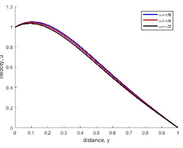
Figure 8: Velocity u for different values of α
39
40
41
Figure 12: Velocity u for different values of m42
43
44
Figure 16: Velocity w for different values of α
45
Figure 18: Velocity w for different values of Grc
46
47
Figure 21: Velocity w for different values of ω49
5.2 ObservationsIt has been observed from figure 10 and 12 that primary velocity ( u ) increases when Gr and m are increased. It means Hall current has increasing effect on the flow of the fluid along the plate. However figure 8, 9, 11, 13, 14 and 15 show that (u) decreases when α, ω, M, Grc, Pr and Sc are increased.
Figure 17, 18 and 19 show that, secondary velocity (w) decreases when Gr, Grc and M are increased. however figure 16, 20 , 21, 22 and 23 show that ( w) decreases when α, ω, m, Grc, Pr and Sc are increased.This shows that the Hall parameter slows down the transverse velocity.
Its observed that concentration reduces with increase in Sc and temperature reduces with increase in Pr .
5.3 Conclusion
The results of the model can have been tested form the graphs represented and support MHD flow. The effect of Hall current is observed on both the primary and secondary
velocities. It has been observed that the primary velocity increases with Hall parameter on the other hand secondary velocity decreases when Hall parameter is increased.
5.4 RECOMENDATION
50
REFERENCESAttia, H., 2002. Unsteady MHD flow and heat transfer of dusty fluid between parallel plates with variable physical properties. Applied Mathematical Modelling, 26, 9: 863–875.
Choi, U.S. (1995) Enhancing Thermal Conductivity of Fluids with Nanoparticles, Developments and Application of Non-Newtonian Flows. ASME Journal of Heat Transfer, 66, 99-105
Datta, N. and Jana, R. N., 1976. Oscillatory magneto hydrodynamic flow past a flat plate with Hall effects. Journal of the Physical Society of Japan, 40, 5: 1469-1474.
Deka, R. K., 2008. Hall effects on MHD flow past an accelerated plate.Theoretical and Applied Mechanics, 35, 4: 333-346.
Devika, B., Satya Narayana,P.V., and Venkataramana, S.2013.MHD Oscillatory flow of a visco elastic fluid in a porouschannel with chemical reaction.International Journal of Engineering Science Invention, 2, 2: 26-35.
Kafousias, N. G.and Raptis, A. 1981. Mass transfer and free convection effects on the flow past an accelerated vertical plate with variable suction or injection. Revue Roumaine des Sciences Techniques, Serie de MecaniqueAppliquee, 26:11-22.
Lighthill On sound generated aerodynamically II. Turbulence as a source of sound (1148): 1–32
Muthucumaraswamy, R. and Janakiraman, B. 2008, Mass transfer effects on isothermal vertical oscillating plate in the presence of chemical reaction.International Journal of Applied Mathematics and Mechanics, 4, 1: 66–74.
Rajput, U. S. and Kumar, S.2013.Radiation effect on MHD flow through porous media past an impulsively started vertical plate with variable heat and
51
Rajput, U. S. and Kumar,S.2011. MHD flow past an impulsively started vertical plate with variable temperature and mass diffusion.Applied Mathematical Sciences,5, 3: 149-157.
Raptis and Kafousias(1982) Magnetohydrodynamic free convective flow and mass transfer through a porous medium bounded by an infinite vertical porous plate
with constant heat flux, 60(12): 1725-1729
Satya Narayana, P. V., Venkateswarlu, B., and Devika, B.2015. Chemical reaction and heat source effects on MHD oscillatory flow in an irregular channel.Ain Shams Engineering Journal, in press.
Satya Narayana, P.V., Rami Reddy, G. and Venkataramana, S. 2011.Hall current effects on free convection MHD flow past a porous plate. International Journal of Automotive and Mechanical Engineering, 3, 350-363.
Satya Narayana, P.V., Venkateswarlu, B. and Venkataramana, S. 2013.Effects of Hall current and radiation absorption on MHD micropolar fluid in a rotating system.Ain Shams Engineering Journal, 4, 4:843-854.
Sharma, S. and Deka, R. K.2012. Thermal radiation and oscillating plate temperature effects on MHD unsteady flow past a semi-infinite porous vertical plate under suction and chemical reaction.International Journal of Physics and
Mathematical Sciences, 2, 2: 33-52.
Sudhakar,K.,Srinivasa Raju, R. and Rangamma, M. 2013. Hall effecton unsteady MHD flow past along a porous flat plate with thermal diffusion, diffusion thermo and chemical reaction.International Journal of Physical and Mathematical Sciences.4, 1:370-395.
U.S.Rajput and Neetu Kanaujia, 2016. MHD flow past vertical plate with variable temperature and mass diffusion in the presence of hall current. International journal of applied science and engineering, 14,2:115-123