WAVEGUIDE AS A NEAR-FIELD MEASURING PROBE OF THE TWO-ELEMENT ARRAY RADIATOR
S. Paramesha
Department of E & C
AIT, Chikmagalur- 577102, Karnataka, India
A. Chakrabarty
Department of E & ECE
IIT, Kharagpur-721302, West Bengal, India
Abstract—In the analysis, an open-ended rectangular waveguide in an infinite groundplane is usedas a near-fieldprobe andthe two-element waveguide array in an infinite groundplane is usedas a radiator. Moment methodanalysis is usedto findthe reflection coefficient of the array element andprobe voltage. The reflection coefficient of the array element, which is also an open-endof a rectangular waveguide, is computedandcomparedwith the reflection coefficients, when the probe is at different positions in the near-field. The computations have also been carriedout to findthe inducedprobe voltage, when the probe scan in transverse plane (planar scanning) at a distance z1 from the
radiator. Goodagreement is obtainedbetween measuredandMOM results.
1. INTRODUCTION
The radiating waveguide is a fundamental electromagnetic structure, andone about which a great deal is known. With the realization of large-scale microwave arrays, the subject of waveguide radiation and mutual coupling has arousedrenewedinterest. The waveguide elements in two-element array in an infinite groundplane being usedas radiating elements are assumedto be excitedin the dominant TE10 mode. An
multiple reflections between radiator and probe, and also mutual coupling effect between radiating elements into account.
The fieldis describedas a sum of M number of weightedsinusoidal basis functions, defined over the extent of the aperture at the plane of the waveguide. This field can be considered to be a magnetic current source which scatteredsome fieldinto the free space andsome fieldis scatteredwithin the waveguide. The tangential components of the scatteredmagnetic fieldwithin the waveguide and that scattered into the free space must be continuous at the plane of the aperture. Enforcement of this boundary condition leads to an integral equation involving the M unknowns used to describe the aperture electric field. This is transformedinto a matrix equation by taking moments with entire domain sinusoidal weighting functions [1]. A solution of this matrix equation provides the values of the unknown coefficients. The fields scattered inside and outside the waveguide are obtained in terms of these coefficients. Assuming a matcheddetector, the power received by the detector and the voltage measured by the measuring device are calculated.
2. FORMULATION OF THE PROBLEM
The geometry of the problem is a measuring waveguide probe at the near-fieldof a two-element waveguide array radiator and it is shown in Figure 1. The aperture dimension of each waveguide is 2a×2b.
The incident magnetic fields at the radiating waveguide apertures 1 and2 for the dominant TE10 mode are given by:
Hxinc1 = −Y0cos
πx 2a
e−jβz (1)
Hxinc2 = −Y0cos
πx 2a
e−jβz =Hxinc1 (2)
and the electric fields at the radiating apertures 1 and 2 are described by:
−→
E1(x, y,0) = uy M
p=1E 1
pe1p (3) −→
E2(x, y,0) = uy M
p=1E 2
pe2p (4)
where the entire domain basis functions ep (p = 1, 2, . . ., M) are defined by
e1p =
sin pπ
2a(x+a)
−a≤x≤a
−b≤y≤b
0 elsewhere
= e2p (5)
The equivalent magnetic current at aperture 1 for computing the externally radiatedmagnetic fieldusing the plane-wave spectrum approach is given by [2]:
−→
Me1 = 2−→E1(x, y,0)×uz = ux
M p=12E
1
psin
pπ
2a(x+a)
−a≤x≤a
−b≤y≤b (6)
The electric vector potential−→F1 at any point in space due to magnetic
current at aperture 1 is given by:
−→
F1 =
aper −→
M1
ee−jk|r−r
|
4π|r− r| ds
(7)
From the identity [3]:
e−jk|r−r|
|r−r| =
1 2πj
∞
−∞ ∞
−∞
ej{(x−x)kx+(y−y)ky−(z−z)kz} kz
The electric andmagnetic fields at any point in space are given by −→
E1 = −∇ ×−→F1 (9)
−→
H1 = −∇ × −→
E1
jωµ =
1
jkη∇ × ∇ ×
−→
F1 (10)
From Equations (2) through (10), the externally scatteredmagnetic fieldat the plane of the aperture 1 (z= 0) is obtainedas:
−→Hext1= 1
2πkη ∞ −∞ ∞ −∞
k×k× −→εs×uz kz
ej(kxx+kyy)dk
xdky
where−→ε1s is the Fourier Transform of the aperture electric field −→Es1; it is given by
−→
ε1s =uxεx1 +uyε1y = 1 2π
Aperture
Es1(x, y,0)e−j(kxx+kyy)dxdy (11)
Therefore, the x-component of the magnetic fieldis given by
Hxext1 = −1 2πkη ∞ −∞ ∞ −∞
kxkyε1x+
k2−k2xε1y kz
ej(kxx+kyy)dk
xdky (12)
Substituting Equation (11) in (12) andsimplifying, we obtain
Hxext11 = − ab
π2kη
M
p=1 Ep1
∞ −∞ ∞ −∞
k2−kx2
k2−k2
x−k2y
1/2sinc(kyb)
jsin(kxa) p even cos(kxa) p od d
pπ 2 1−
2akx
pπ
2 e
j(kxx+kyy)dk
xdky (13)
aperture 2 is obtainedas:
Hxext22 = − ab
π2kη
M
p=1 Ep2
∞ −∞ ∞ −∞
k2−kx2
k2−k2
x−k2y
1/2sinc(kyb)
jsin(kxa) p even cos(kxa) p od d
pπ 2 1−
2akx
pπ
2 e
j(kxx+kyy)dk
xdky (14)
The internally scatteredfieldat the waveguide aperture is obtainedby using the modal expansion approach [3]. Thex-component of the internally scatteredmagnetic fields at apertures 1 and2 are obtainedas:
Hxint1 = M
p=1
Ep1Ype0sin mπ
2a(x+a)
(15)
Hxint2 = M
p=1
Ep2Ype0sin mπ
2a(x+a)
(16)
The externally radiated x-component of the magnetic fields at the plane of the probe’s aperture due to the radiating apertures 1 and 2 are obtainedas:
Hxext31 = − ab
π2kη
M
p=1 Ep1
∞ −∞ ∞ −∞
k2−kx2
k2−k2
x−k2y
1/2sinc(kyb)
jsin(kxa) p even cos(kxa) p od d
pπ 2 1−
2akx
pπ
2 e
j(kxx+kyy−kzz)dk
xdky (17)
Hxext32 = − ab
π2kη
M
p=1 Ep2
∞ −∞ ∞ −∞
k2−kx2
k2−k2
x−k2y
1/2sinc(kyb)
jsin(kxa) p even
cos(kxa) p od d pπ 2 1−
2akx
pπ
2 e
j(kxx+kyy−kzz)dk
where superscript 3 indicates the probe aperture. Thex-component of the magnetic fieldat the plane of the probe aperture scatteredby the magnetic current on the probe is the same form as the Equation (13) (or (14)). In addition, thex-component of the magnetic fields, at the plane of the radiating waveguide apertures 1 and 2 scattered by the magnetic current on the probe are same form as Equations (17) and (18), respectively.
The boundary conditions are simultaneously imposed at the plane of the radiating waveguide apertures 1 and 2, and at the plane of the near-field probe’s aperture. The boundary condition at the region of the waveguide aperture is the tangential component of the magnetic field both inside the waveguide and outside it should be identical.
Atz= 0 plane, thex-component of the magnetic fieldat the plane of the radiating aperture 1 is given by:
2Hxinc1+Hxint1=Hxext11+Hxext12+Hxext13 (19)
The x-component of the magnetic fieldat the plane of the radiating aperture 2 is given by:
2Hxinc2+Hxint2=Hxext22+Hxext21+Hxext23 (20)
At z = z1 plane, the x-component of the magnetic fieldat the
plane of the measuring probe’s aperture is given by:
Hxint3=Hxext33+ 2Hxext31+ 2Hxext32 (21)
Since the fieldis describedby M basis functions, M unknowns are to be determined from the boundary condition. The Galerkin’s specialization of the methodof moments is usedto obtainM different equations from the boundary condition to enable the determination of theEp. The weighting functionwq is selectedto be of the same form as the basis function ep. The integral Equations (19), (20) and(21) are then convertedinto matrix form as:
2Linc1+Lint1Ep1=Lext11Ep1+Lext12Ep2+Lext13Ep3
(22)
2Linc2+Lint2Ep2=Lext22Ep2+Lext21Ep1+Lext23Ep3
(23)
Lint3 Ep3=Lext33 Ep3+Lext31 Ep1+Lext32 Ep2 (24)
as:
Linc1 = Lincq 1=Hxinc1, w1q=
−2abY0 q= 1
0 otherwise
(25)
Lint1 = Lintq,p1=Hxint1(e1p), wq1=
2abYe
p p=q =m &n= 0 0 otherwise
(26)
Lext11 = Lextq,p11=Hxext11(e1p), wq1
= −4a
2b2
π2kη ∞ −∞ ∞ −∞
k2−k2
x
k2−k2
x−ky2
1/2sinc 2(k
yb)
sin2(kxa) p,q both even cos2(kxa) p,q both odd 0 otherwise pπ 2 1− 2akx
pπ 2 qπ 2 1− 2akx
qπ
2dkxdky (27)
Lext12=Lextq,p12=Hxext12(e2p), w1q
=−4a
2b2
π2kη ∞ −∞ ∞ −∞
k2−k2
x
k2−k2
x−k2y
1/2sinc 2(k
yb)
sin2(kxa) p,q both even cos2(kxa) p,q both odd
0 otherwise pπ 2 1−
2akx
pπ
2qπ
2
1−
2akx
qπ
2e
−j(kxx1+kyy1)dk
xdky
(28)
Lext13=Lextq,p13=Hxext13(e3p), w1q
=−4a
2b2
π2kη ∞ −∞ ∞ −∞
k2−kx2
k2−k2
x−k2y
1/2sinc 2(k
sin2(kxa) p,q both even cos2(k
xa) p,q both odd 0 otherwise
pπ
2
1−
2akx
pπ
2 qπ
2
1−
2akx
qπ
2
e−j(kxx1+kyy1+kzz1)dkxdky (29)
The expressions forLinc2 is the same form as Equation (25),
Lint2and Lint3are the same form as Equation (26), Lext22 and
Lext33 are the same form as Equation (27), Lext21 is the same as Equations (28) andLext23,Lext31andLext32are the same form as Equation (29). Solving Equations (22), (23) and(24) simultaneously, we obtain the coefficients of the basis functions E1
p,Ep2 and Ep3. From these coefficients, radiating element reflection coefficient and power receivedby the probe andhence the voltage are determined. The expression for power coupledinto the probe waveguide in the TE10
mode is given by [4]:
P = 2abY0Ep3Ep3∗ (30)
Since measuring devices viz. spectrum analyzer has an input impedance of 50 ohms, the voltage is given by:
V =√50×Pvolts (31)
3. RESULTS AND DISCUSSION
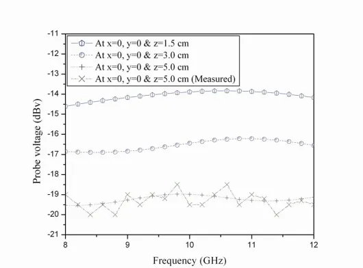
Figure 2. Probe voltage inx-yplane atx= 0 andz= 0.5λ/1.0λ/2.0λ, andat 10 GHz, when separation between radiating elements is d = 2.54 cm.
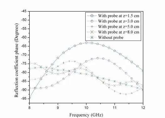
Figure 4. Absolute reflection coefficient for the radiating array element in the presence of the probe at x = 0, y = 0 and z = 1.5 cm/3.0 cm/5.0 cm/8.0 cm, and in the absence of the probe over 8 to 12 GHz when the separation between radiating elements isd= 2.54 cm.
separation between radiating elements d is 2.54 cm. When the probe is closer to the radiator, the reflection coefficient reduces, as it makes the better matching between radiator and probe. These are compared with the reflection coefficient of the radiating elements when there is no probe at the near-field. The reflection coefficient phase plots are shown in Figure 5.
4. CONCLUSION
When the radiating elements and probe are open-ended waveguides, because of multiple reflections and mutual coupling effect, and equivalent circuit properties of dominant mode the radiating element reflection coefficient improves. When the distance between probe and radiator reduces, the reflection coefficient decreases drastically, and the probe voltage increases, as evident from the plots. When the distance between the radiator and probe is larger, then the reflection coefficient values tend to the results obtained when there is no probe at the near-field.
REFERENCES
1. Harrington, R. F., Field Computation by Moment Method, Roger E. Krieger Publishing Company, USA, 1968.
2. Paramesha, S. and A. Chakrabarty, “Moment method analysis of rectangular waveguide as near-field measuring probe,”Microwave and Optical Technology Letters, Vol. 48, No. 9, September 2006. 3. Harrington, R. F., Time-Harmonic Electromagnetic Fields,
McGraw-Hill, New York, 1961.