FRACTIONALLY SPACED CONSTANT MODULUS ALGORITHM FOR WIRELESS CHANNEL
EQUALIZATION
A. Kundu and A. Chakrabarty
Kalpana Chawla Space Technology Cell (KCSTC)
Department of Electronics and Electrical Communication Engineering Indian Institute of Technology
Kharagpur-721 302, West Bengal, India
Abstract—Wireless channel identification and equalization is one of the most challenging tasks because broadcast channels are often subject to frequency selective, time varying fading and there are several bandwidth limitations. Furthermore, each receiver channel has vastly different types of channel characteristics and signals to noise ratio. Here in this paper we consider channel equalization and estimation problem from trans-receiver perspective, specifically we try to estimate blind equalization schemes particularly using constant modulus Algorithm (CMA). We try to estimate a linear channel model driven by a QAM source and adapt a FSE (T /2) using CMA. It has been shown CMA-FSE successfully reduces the cluster variance so that transfer to a decision directed mode is possible and simultaneously error is reduced.
1. INTRODUCTION
from a finite M array real alphabet of zero mean means all symbols are equally probable.
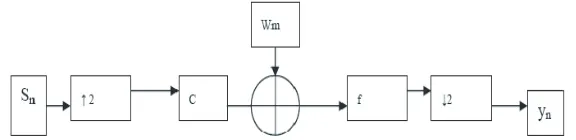
Figure 1. T /2spaced multirate system model with added interference.
Here in Fig. 1, Sn implies baud spaced source symbol at sample index n, c is the vector representing the fractionally spaced channel impulse response. w is the additive white Gaussian channel noise, f represents vector containing the fractionally spaced equalizer coefficients. yn is the baud spaced equalizer output. No of coefficients in the channel and equalizer response vectors are Nc and
Nf respectively. The system output can be expressed as
yn=sT(n)Cf+wT(m)f (1)
where s(n) = [sn, sn−1, . . . , sn−Ns+1]
T is the length N s = [(Nc+Nf −1)/2] vector of baud spaced source symbols w(m) = [wm, wm−1, . . . , wm−Nf+1]
T is the vector of additive zero mean white Gaussian noise with varianceσωandCis theNs∗Nf decimated channel convolution matrix given by
C=
c1. . . c0
. . . c1. . . c0 . . . .
cNc−1cNc−2. . . .
. . . cNc−1·cNc−2
2. CONSTANT MODULUS ALGORITHM
The CMA criterion may be expressed by the non negative cost function
JCMAp,q parameterized by positive integer p andq.
JCMAp,q =
1
pqE{||ya|
p−γ|q}
(2)
in the amplitude of output that otherwise has a constant modulus. For simplest case we putp= 2 &q= 2. It updates weights by minimizing the cost function. The steepest gradient descent algorithm [13–15, 19] is obtained by taking the instantaneous gradient of JCMAp,q which
results equation which updates the system.
f(n+ 1) = f(n)−µg(w(n)) (3)
g(w(n)) = r∗(n)ψ(yn) (4)
ψ(yn) = −∇yn
1 4
|yn|2−γ 2=yn
γ− |yn|2 (5)
where f is the length Nf is equalizer coefficient vector, r(n) is the length-Nf receiver input vector, µ is small step size and ψ(yn) is the CM error function for CMA2,2. Whereγ is taken as
γ =E
|Sn|4
/E
|Sn|2
(6)
To improve computational efficiency a signed error algorithm used to modify the update equation of the channel equalizer. Here we took only the sign of the error function there simplified by eliminating multiply operation. The Equation (3) modified as
f(n+ 1) =f(n)−µr(n)sgn(ψ(yn)) (7) This modified CMA known as SE-CMA is equivalent to CMA1,1. Now
we consider CMA1,1 cost function
JCMA1,1 =E{||yn| −β|} (8)
and corresponding update equation
f(n+ 1) =f(n)−µr(n)sgn(yn(β− |yn|)) (9) When β =√γ, the CMA1,1 update equation is identical to SE-CMA
so (8) becomes
JSE−CMA =E{||yn| −√γ|} (10)
Selection of γ is important because of the systems convergence. The dissipation constant γ should be chosen such that the γ = a2
v where
av is the vth positive member of the source alphabet and integer v satisfies
v= arg mink
k−1/2
1 +√M2/2−1 2
For BPSK γ is taken as 1 and for 8 PAM γ is taken as 9/5 for satisfactory result. The cost function of SE-CMA depends on the following terms s, C, f,γ,M,Ns, σω. S is the set of all MNs source symbol possibilities. For a system with BPSK source, a channel length of 6 and an equalization length of 2(M = 2 ;Nc = 6;Nf = 2 ;Ns= 3). The set of possible symbol combination is
S= 1 1 1 , 1 1 −1 , 1 −1 1 −1 1 1 −1 1 −1 −1 −1 1 , −1 −1 −1 We know
erf(x) = √2
π
x
0
exp−t2dt (12)
and
Q(t) = √1 2π ∞ x exp
−t2 2
dt (13)
JSE−CMA = E{||yn| −√γ|}=EsTCf+wTf−√γ (14)
After full expansion the expression comes as
JSE−CMA = M−Ns
n∈s
−√γ−4√γ+sTCfQ
√
γ+sTCf
σω f 2
+2sTCf Q
sTCf
σω f 2
+
2
πσω f 2
2exp
−
√
γ+sTCf2 2σ2
ω f 22
−exp
−
sTCf2 2σ2
ω f 22
(15)
3. CHANNEL MODEL FOR A QAM SOURCE
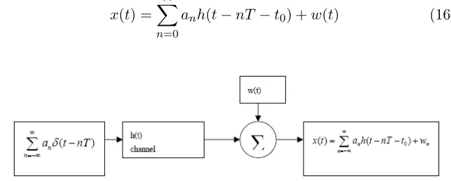
Channel output of a QAM communication system described by equation
x(t) =
∞
n=0
anh(t−nT −t0) +w(t) (16)
Figure 2. Channel model for a QAM.
Figure 2shows a sequence of independent identically distributed complex data {an} is sent by the transmitter over a LTI channel with impulse response h(t). The receiver attempts to recover the input data sequence{an}for measurable channel outputx(t) in which
T is the symbol period. The channel output may be corrupted by
w(t) channel noise which is zero mean stationary, white and complex Gaussian with varianceσ2and is independent of the channel inputan. Assume the complex data and noise both satisfy symmetric property
Ea2n= Ew2t = 0 in additionE
|an|4
−2E2
|an|2
<0, i.e., the kurtosis K(an) of an is negative as is often the case of QAM system. When the distortion caused by channel (LTI [10, 11], non ideal) is significant, equalization is needed to remove the ISI [20] at the sampling instants (t = nT). Due to the presence of ISI, the recovery of input signal sequenceanrequires that the channel impulse responseh(t−T0) be identified either explicitly or in decision feedback
equalization (DFE) [9, 20] or implicitly as in linear equalization. In traditional blind equalization system the channel output sampled at the known baud rate 1/T. The sampled channel output
x(nT) =
∞
k=0
akh(nT −kT−t0) +w(nT)
=anh(nT −t0) +w(nT)
is a stationary process, using this notations xn
∆
= x(nT); wn
∆
=
w(nT);hn =∆ h(nT −t0) the previous equation can be written as
discrete convolution with noise
xn=
∞
k=−∞
akhn−k+wn (18)
Based on this relationship traditional linear TSE are designed as FIR
filter θ(z−1) = N
k=0
θkz−k to be applied on xn to remove the ISI from the equalizer outputyn=
N
k=0
θkxn−k. Most of the equalizer algorithm proposes to adjust the parameter{θk}Nk=0. CMA aims to minimize the cost function given in (19).
J2(θ) =
1 4E
|yn|2−R2
2
R2=
E
|an|4
E
|an|2
(19)
If we wish to maximize|K(yn)|it requiresEy2n=Ea2nwhereK(yn) is kurtosis of signalyn.
|K(yn)|
∆
=E
|yn|4
−2
E
|yn|2 −Eyn22 (20) From the Fig. 3 it is apparent that x(t) is a continuous time cyclostationary process with periodT as long as the channel bandwidth is greater than the minimum BW 1/2T. Let sampling interval ∆ = PT; sampled channel outputx(k∆) = ∞
n=0
anh(k∆−np∆−t0) for p >1,
the over sampled channel output x(k∆) can be divided into p sub-sequences. x(ki)=∆x[(kp+i)∆] =x(kT+i∆), i= 1, . . . , p.By defining the sub-channel impulse response ash(ki)=∆ h(pk∆ +i∆−t0) =h(kT+ i∆−t0); thepsub-sequence can be written asx(ki) =
+∞
n=0
anhik−n+w
(i)
k , thesepsub-sequences can be viewed as stationary outputs ofpdiscrete
FIR channels. Hi(z) = K
k=0 hi
H1(Z)
H2(Z)
Hp(Z)
2( )z
θ
( )
pz θ
n
a
Yn
1( )z
θ
CMA
p n
y
1 n
y
an
Descision
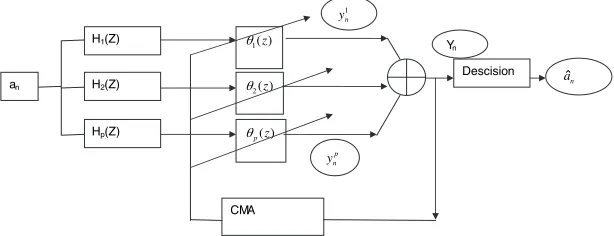
Figure 3. Multichannel vector representation of blind adaptive FSE.
One adjustable filter [8] is provided for each sub-sequences x(ki), thus the actual equalizer is a vector of filters. θi(z) =
N
k=0
θ(ki)z−k, i =
1, . . . , p. The p stationary filter output
yn(i)
are summed to form the stationary equalizer output
yn=
p
i=1
yn(i) (21)
Define FSE parameter asθ= [∆ θ0(1), θ(1)N , θ(0p), . . . , θN(p)]. To adaptively adjust θ without a training sequence, CMA can be implemented to jointly update the p filters to minimize cost function. From cost function we obtain stochastic gradient algorithm as follows
θ(ki)(n+ 1) =θk(i)(n)−µx(ni−)kyn
|yn|2−R2 , i= 0,1, . . . , p−1;
(22)
where µ is small step size and θk(i) is the kth coefficient of the ith filter at the nth iteration. This combination of CMA & FSE used to implement blind adaptive algorithm for equalizer [18].
4. BLIND ADAPTIVE FSE
0 50 100 150 200 250 300 100
Magnitude of Impulse Response Coefficients
0 100 200 300 400 500
0 1 2 3
Frequency Response Magnitude
Figure 4. Frequency response characteristics of channel.
0 1000 2000 3000 4000 5000 10-0.31
10-0.29 10-0.27
iteration vs MSE plot
iteration
mse
e
Figure 5. CMA blind equalizer performance with 16 QAM, step size = 0.001, SNR at equalizer input 35 dB.
Variables section, and the channel is selected in the Channel section of the code. The CMA-FSE successfully reduces the cluster variance so that transfer to a Decision Directed mode is possible, further error rate reduction is desired. Simulated results demonstrate CMAs ability to adapt a FSE blindly from a received sequence synthesized from a shortened version (length-16). The source is 16 QAM, white and equiprobable. The equalizer is length-16 and initialized with a unity center spike and all other taps zero, and the step-size is 0.001. The
f 0
f1
CMA Error Surface
MSE ellipse axes
-3 -2 -1 0 1 2 3 -1
-0.5 0 0.5 1
Figure 6. CM Cost Surface plots over equalizer plane for length-2 real-valued channels.
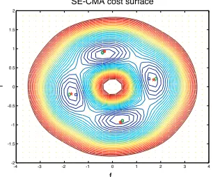
SE-CMA cost surface
f0
f1
-4 -3 -2 -1 0 1 2 3 4
-2 -1.5 -1 -0.5 0 0.5 1 1.5 2
SNR at the equalizer input is 35 dB. The received signal is normalized to (near) unity power.
The convergence of equalizer parameter vector under CMA can be viewed as a transverse of the CMA cost surface [2, 5, 6, 8] with average movement in the direction of steepest descent, so from the Fig. 6 dynamical behavior of CMA can be estimated.
-1 -0.8 -0.6 -0.4 -0.2 0 0.2 0.4 0.6 0.8 1 -30 -20 -10 0 10 dB
normalized to baud frequency Channel, equalizer frequency response magnitudes
-0.5 0 0.5
-1.5 -1 -0.5 0
dB
normalized to baud frequency System frequency response magnitude
channel eq
mmse-glob
sysmmse-glob
Figure 8. Frequency re-sponse analysis of 6 tap, T /2 fractionally-spaced, 16 QAM source, equalizer length 2, SNR 50 dB, step size 5e−3, no of iteration 5000.
0 1000 2000 3000 4000 5000
-6 -4 -2 0 2
Smoothed CM-error history
iteration number
dB
0 1000 2000 3000 4000 5000
-10 -5 0 Squared-error history iteration number dB MSE mmse-loc MSE mmse-glob
Figure 9. Plot of smoothed CM error history and variation of square error with iteration.
0 1000 2000 3000 4000 5000 0
0.5
1 Equalizer coefficient histories
iteration number
real
0 1000 2000 3000 4000 5000 -0.1
0 0.1
iteration number
imag
Figure 10. Plot of CMA equalizer coefficient history with iteration.
0 500 1000 1500 2000 2500 3000 3500 4000 4500 5000 -0.6 -0.4 -0.2 0 0.2 0.4 0.6 0.8
Equalizer coefficient histories
iteration number
real
0 500 1000 1500 2000 2500 3000 3500 4000 4500 5000 -0.4 -0.2 0 0.2 0.4 0.6 iteration number imag
Figure 11. SE-CMA equalizer coefficient history with iteration.
corresponding wiener solutions since CM criterion operates purely on the magnitude of the equalizer output not the phase shift of adaptive filter.
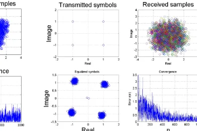
Figure 12. Transmitted symbol, received and equalized symbol, convergence plot with iteration for CMA.
Figure 13. Transmitted symbol, received and equalized symbol, convergence plot with iteration for FSE-CMA.
5. CONCLUSION
REFERENCES
1. Brown, D. R., P. B. Schniter, and C. R. Johnson, Jr., “Computationally efficient blind equalization,” 35th Annual
Allerton Conference on Communication, Control, and Computing,
September 1997.
2. Godard, D. N., “Self-recovering equalization and carrier tracking in two-dimensional data communication systems,” IEEE Trans.
on Communications, Vol. 28, No. 11, 1867–1875, November 1980.
3. Casas, R. A., C. R. Johnson, Jr., R. A. Kennedy, Z. Ding, and R. Malamut, “Blind adaptive decision feedback equalization: A class of channels resulting in ill-convergence from a zero initialization,” International Journal on Adaptive Control and
Signal Processing Special Issue on Adaptive Channel Equalization,
Vol. 12, No. 2, 173–193, March 1998.
4. Fijalkow, I., C. E. Manlove, and C. R. Johnson, Jr., “Adaptive fractionally spaced blind CMA equalization: Excess MSE,”IEEE
Trans. on Signal Processing, Vol. 46, No. 1, 227–231, 1998.
5. Johnson, Jr., C. R. and B. D. O. Anderson, “Godard blind equalizer error surface characteristics: White, zero-mean, binary source case,”International Journal of Adaptive Control and Signal
Processing, Vol. 9, 301–324, July–August 1995.
6. Ding, Z., R. A. Kennedy, B. D. O. Anderson, and C. R. John-son, Jr., “Ill-convergence of godard blind equalizers in data com-munication systems,” IEEE Trans. on Communications, Vol. 39, 1313–1327, September 1991.
7. Johnson, Jr., C. R., S. Dasgupta, and W. A. Sethares, “Averaging analysis of local stability of a real constant modulus algorithm adaptive filter,” IEEE Trans. on Acoustics, Speech, and Signal
Processing, Vol. 36, 900–910, June 1988.
8. Walsh, J. M. and C. R. Johnson, Jr., “Series feedforward inter-connected adaptive devices,” Proc. the International Conference
on Acoustics, Speech, and Signal Processing (ICASSP), Montreal,
Quebec, May 2004.
9. Al-Kamali, F. S., M. I. Dessouky, B. M. Sallam, and F. E. Abd El-Samie, “Frequency domain interference cancellation for single carrier cyclic prefix cdma system,” Progress In Electromagnetics
Research B, Vol. 3, 255–269, 2008.
11. De Doncker, P., “Spatial correlation functions for fields in three-dimensional rayleigh channels,” Progress In Electromagnetics
Research, PIER 40, 55–69, 2003.
12. Andalib, A., A. Rostami, and N. Granpayeh, “Analytical inves-tigation and evaluation of pulse broadening factor propagating through nonlinear optical fibers (traditional and optimum disper-sion compensated fibers),”Progress In Electromagnetics Research, PIER 79, 119–136, 2008.
13. Xue, W. and X.-W. Sun, “Multiple targets detection method based on binary hough transform and adaptive time-frequency filtering,” Progress In Electromagnetics Research, PIER 74, 309– 317, 2007.
14. Wilton, D. R. and J. E. Wheeler III, “Comparison of convergence rates of the conjugate gradient method applied to various integral equation formulations,” Progress In Electromagnetics Research, PIER 5, 131–158, 1991.
15. Chen, K.-S. and C.-Y. Chu, “A propagation study of the 28 GHz lmds system performance with M-QAM modulations under rain fading,”Progress In Electromagnetics Research, PIER 68, 35–51, 2007.
16. Lundstedt, J. and M. Norgren, “Comparison between frequency domain and time domain methods for parameter reconstruction on nonuniform dispersive transmission lines,” Progress In
Electromagnetics Research, PIER 43, 1–37, 2003.
17. Oraizi, H. and S. Hosseinzadeh, “A novel marching algorithm for radio wave propagation modeling over rough surfaces,” Progress
In Electromagnetics Research, PIER 57, 85–100, 2006.
18. Mukhopadhyay, M., B. K. Sarkar, and A. Chakrabarty, “Augmentation of anti-jam GPS system using smart antenna with a simple doa estimation algorithm,”Progress In Electromagnetics
Research, PIER 67, 231–249, 2007.
19. Kazemi, S., H. R. Hassani, G. Dadashzadeh, and F. Geran, “Performance improvement in amplitude synthesis of unequally spaced array using least mean square method,” Progress
In Electromagnetics Research B, Vol. 1, 135–145, 2008.
doi:10.2528/PIERB0710300
20. Al-Kamali, F. S., M. I. Dessouky, B. M. Sallam, and F. E. Abd El-Samie, “Frequency domain interference cancellation for single carrier cyclic prefix CDMA system,”Progress In Electromagnetics