Development of a 1-Dimensional Data Assimilation to Determine Temperature and Relative Humidity Combining Raman Lidar Backscatter Measurements And a Reanalysis Model

(1)

Scholarship@Western

Electronic Thesis and Dissertation Repository

7-30-2019 10:00 AM

Development of a 1-Dimensional Data Assimilation to Determine

Temperature and Relative Humidity Combining Raman Lidar

Backscatter Measurements And a Reanalysis Model

Shayamila N. Mahagammulla Gamage

The University of Western Ontario

Supervisor Robert Sica

The University of Western Ontario Co-Supervisor Alexander Haefele

The University of Western Ontario Graduate Program in Physics

A thesis submitted in partial fulfillment of the requirements for the degree in Doctor of Philosophy

Follow this and additional works at: https://ir.lib.uwo.ca/etd

Part of the Atmospheric Sciences Commons, Meteorology Commons, Statistical Methodology Commons, and the Statistical, Nonlinear, and Soft Matter Physics Commons

Recommended Citation Recommended Citation

Mahagammulla Gamage, Shayamila N., "Development of a 1-Dimensional Data Assimilation to Determine Temperature and Relative Humidity Combining Raman Lidar Backscatter Measurements And a Reanalysis Model" (2019). Electronic Thesis and Dissertation Repository. 6356.

https://ir.lib.uwo.ca/etd/6356

This Dissertation/Thesis is brought to you for free and open access by Scholarship@Western. It has been accepted for inclusion in Electronic Thesis and Dissertation Repository by an authorized administrator of

(2)

Abstract

Water vapor is the most dominant greenhouse gas in Earth’s atmosphere. It is highly variable

and its variations strongly depend on changes in temperature. Atmospheric water vapor can

be expressed as relative humidity (RH), the ratio of the partial pressure of water vapor in

the mixture to the equilibrium vapor pressure of water over a flat surface of pure water at a

given temperature. Liquid water can exist as super-cooled water for temperatures between

0◦_{C to}₋₃₈◦_{C. Thus, RH can be measured either relative to water (}_RH_{w) or to ice (}_RH_i). _RH

i

measurements are important in the upper tropospheric region, where the temperature is always

less than 0◦_{C, to study ice supersaturation (ISS) and its relation to the formation of cirrus}

clouds.

I present three studies all using a mathematical scheme called the optimal estimation method

(OEM). The OEM is an inverse method that determines the most probable state consistent with

the measurements and a priori knowledge. These studies use parts of a large set of existing

measurements from the Raman Lidar for Meteorological Observations (RALMO) instrument

located at the meteorological observatory in Payerne, Switzerland.

I first develop an OEM retrieval for temperature using RALMO’s two pure rotational

Ra-man (PRR) channel measurements. Retrieved temperatures show excellent agreement with

coincident balloon-borne radiosonde measurements. A second OEM scheme is introduced to

retrieveRHw directly from RALMO measurements of back-scatter due to water vapor and

ni-trogen. I validate the OEM retrievals developed for temperature and RHw. I then combine

the OEM-retrieved temperature and RHw with data from the European Centre for

Medium-Range Weather Forecasts Re-analysis (ERA5) to compute a new and improved temperature

and relative humidity product. The retrieval is enhanced by assimilating it with the ERA5 data.

The quality of the RHw retrievals from the assimilated OEM scheme greatly improves over

retrievals which use less accurate a priori information.

Thirdly, I retrieve RHi to detect ISS layers. I find the frequency of ISS layers in the free

troposphere over Payerne to be about 27% using 82.5 hours of measurements.

Keywords: 1D Var Data Assimilation, Reanalysis, Optimal Estimation Method, ERA5,

Raman lidar, Rotational Raman temperature, UTLS, Water vapor mixing ratio, Relative

hu-midity, Ice supersaturation, Particle extinction

(3)

Water vapor is the most dominant greenhouse gas in Earths atmosphere that is highly

vari-able. Variations of the atmospheric water vapor strongly depend on changes in temperature.

Accurate estimates of humidity and temperature and as well as the uncertainties associated

are required for both weather and climate forecasting purposes. I present a new mathematical

and statistical approach to estimate both atmospheric humidity and temperature using Raman

lidar backscatter measurements. The new method provides full uncertainty budgets for each

estimated temperature and relative humidity profile, that represent the errors due to

instrumen-tation, estimation method and so on. I have also combined the Raman lidar measurements into

the data from the ERA5 that is the latest major global reanalysis produced by European

Cen-tre for Medium- Range Weather Forecasts (ECMWF), to enhance the quality of the humidity

and temperature estimates. My results show that the quality of the temperature and

humid-ity retrievals are greatly improved and agree best with the measurements made by coincident

radiosondes.

(4)

Co-Authorship Statement

The entire thesis is written under the supervision of Dr. Robert Sica and Dr. Alexander Haefele.

Main research ideas are generated by Dr. Sica and Dr. Hafele.

I was provided with raw Raman lidar measurements from Raman Lidar for Meteorological

Observations (RALMO) and radiosonde measurements from MeteoSwiss located in Payerne,

Switzerland. Both lidar and sonde measurements have been used in the work presented in

Chapters 2,3, and 4.

The work presented in Chapter 2 was done in collaboration with Dr. Gianni Martucci. The

traditional Raman lidar temperature analysis was performed and provided to me by Dr. Gianni

Martucci. I was provided with the RALMO data processing codes and the OEM codes written

by Dr. Sica and Dr. Haefele in their water vapor and Rayleigh temperature studies. All the

necessary MATLAB codes related to the OEM Raman temperature algorithm were written by

me. I also conducted the OEM analysis for temperature retrievals and compared the results

with the radiosonde and traditional Raman lidar temperatures.

The work done in Chapters 3 and 4 is based on the studies of OEM Raman temperature

study by me and the OEM water vapor mixing ratio by Dr. Sica and Dr. Haefele. In the work

presented in both Chapters 3 and 4, I have used the ERA5 hourly reanalysis data obtained from

the ECMWF data archive. I was responsible for providing the MATLAB codes for the OEM

relative humidity retrievals, and I performed the OEM analysis.

(5)

This work would not be possible without the guidance of my two supervisors Dr. Robert Sica

and Dr. Alexander Haefele. I would thank both for supporting me with my work and providing

me with opportunities to present my work in conferences and various other platforms. I would

like to thank MeteoSwiss in Payerne (the federal Office of Meteorology and Climatology) in Switzerland for allowing me to use the data from their Raman lidar system. Understanding of

the RALMO system and the detection of rotational Raman spectrum was possible thanks to Dr.

Valentine Simeonov of Ecole Polytechnique Federale de Lausanne. I would like to thank Dr.

Gianni Martucci for his invaluable instruction and inputs for my work. Also, I would like to

thank everyone working at MeteoSwiss for their great support and motivation.

This work is not only supported by a MeteoSwiss and Western University but also by

Na-tional Science and Engineering Research Council of Canada and the Canadian Space Agency

under the Arctic Validation and Training for Atmospheric Research in Science (AVATARS)

program.

I also thank the Western writing support center and Patricia Sica for their assistance in

editing and proofreading all my papers and my thesis. I am thankful to my colleague Ghazal

Farhani for being there for me for everything. I would also like to thank Dr. Emily McCullough,

the first person whom showed me how the lidars work and how to make things work. Also, I

am thankful for all the great inputs and support given by my purple crow lidar group members

throughout the years of my PhD.

I am appreciative toward Dr. Blaine A. Chronik and Dr. Aaron Sigut who were on my

academic committee and providing me with great advice and motivation to complete my thesis.

I also thank Dr. Kanthi Kaluarachchi for being a motherly figure to me and guiding me in

many ways to succeed. I thank all the staff at Physics department who were always helpful and supportive. I have no words to thank Rajitha, my roommate for tolerating me for all these

years and I am surely indebted for her support.

Finally, I would like to thank my parents and my sisters. I am thankful for their

uncon-ditional love and support. Everything I achieve in my life including the PhD I would like to

dedicate to my wonderful family.

(6)

List of Figures

1.1 An atmospheric temperature profile based on the US Standard Atmosphere

val-ues showing the regions of the atmosphere based on temperature structure. . . . 9

1.2 The important processes in the UTLS region . . . 11

1.3 Variation with temperature of the saturation vapor pressure over a plane surface

of pure water and the difference between the saturation vapor pressure over a plane surface of water to ice . . . 14

1.4 Schematic drawing of lidar system. . . 19

1.5 The different types of light scattering . . . 22

1.6 Raman backscatter spectrum of the atmosphere for an incident laser wavelength

of 355 nm . . . 23

1.7 Optical diagram of the transceiver of RALMO (PB - Pellin Broka prism).

Adapted from Dinoev et al. (2010). . . 30

1.8 Schematic of the OEM retrieval algorithm . . . 38

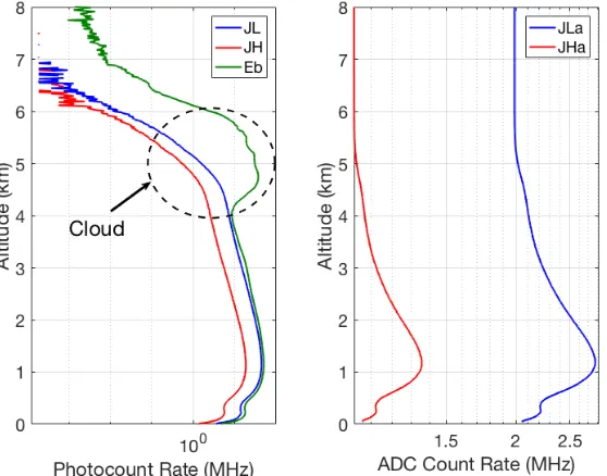
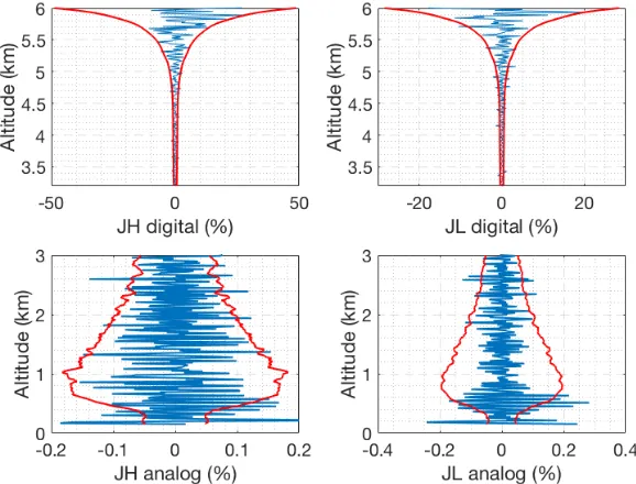
2.1 Count rate for 30 min of coadded RALMO measurements from 2300 UT on 09

September 2011, a clear night . . . 62

2.2 Difference between the forward model and clear nighttime RALMO measure-ments on 09 September 2011 . . . 63

2.3 Averaging kernels and vertical resolution for temperature retrievals from the

clear nighttime RALMO measurements on 09 September 2011 . . . 64

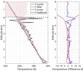
2.4 Retrieved temperature profile and the statistical uncertainty using the OEM

from the clear nighttime RALMO measurements on 09 September 2011 in

comparison with the coincident sonde measurements . . . 65

(11)

measurements on 09 September 2011 . . . 66

2.6 Retrieved geometrical overlap function from the clear nighttime RALMO

mea-surements on 09 September 2011 . . . 67

2.7 Count rate for 30 min of clear coadded RALMO measurements from 1100 UT

on 10 September 2011 . . . 68

2.8 Difference between the forward model and the clear daytime RALMO mea-surements on 10 September 201 . . . 69

2.9 Averaging kernels and vertical resolution for temperature retrievals from the

clear daytime RALMO measurements on 10 September 2011 . . . 69

from the clear daytime RALMO measurements on 10 September 2011 in

com-parison with the coincident sonde measurements . . . 70

2.11 Random uncertainties and systematic uncertainties due to the forward model

parameters for the temperature retrievals from the clear daytime RALMO

mea-surements on 10 September 2011 . . . 71

July 2011 with the presence of a cirrus cloud . . . 72

2.13 Difference between the forward model and the nighttime RALMO measure-ments on 05 July 2011 with the presence of a cirrus cloud . . . 72

2.14 Averaging kernels and vertical resolution for temperature retrievals from

mea-surements on 05 July 2011 with a cirrus cloud at 6 km height . . . 73

from the RALMO measurements on 05 July 2011 with a cirrus cloud at 6 km

height, in comparison with the coincident sonde measurements . . . 73

2.16 The OEM retrieved particle extinction, calculated Backscatter coefficient, and estimated lidar ratio profiles from the RALMO measurements on 05 July 2011

with of a cirrus cloud present at 6 km height . . . 74

(12)

June 2011, which has a cloud base at an height about 4 km . . . 75

2.18 Difference between the forward model and the nighttime RALMO measure-ments on 21 June 2011 with the presence of a lower level cloud . . . 76

2.19 Averaging kernels and vertical resolution for temperature retrievals from

mea-surements on 21 June 2011 with the presence of lower level cloud . . . 77

from the RALMO measurements on 21 June 2011 with the presence of a lower

level cloud, in comparison with the coincident sonde measurements . . . 77

2.21 The OEM retrieved particle extinction, calculated Backscatter coefficient, and estimated lidar ratio profiles from the RALMO measurements on 21 June 2011

with the presence of a lower level cloud . . . 78

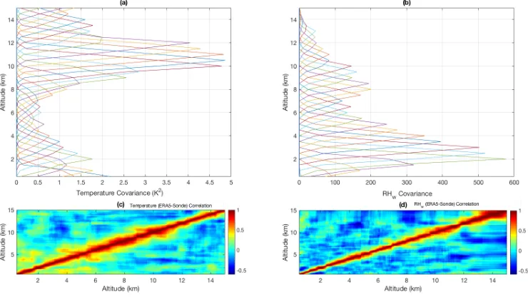
3.1 Dates and times of the sondes were launched from Payerne, Switzerland that

coincide with the ERA5 reanalysis data used to estimate the correlations of the

temperature and relative humidity . . . 94

3.2 Temperature and relative humidity biases of the ERA5 reanalysis data . . . 95

3.3 Covariance and correlation matrices for temperature and relative humidity . . . 95

3.4 The OEM-retrieved temperature and relative humidity profiles, averaging

ker-nels and uncertainty budgets from RALMO measurements on 28 August 2012

with 30 min temporal and 90 m vertical resolutions . . . 99

3.5 The OEM-retrieved temperature and relative humidity profiles, averaging

ker-nels and uncertainty budgets from RALMO measurements on 10 September

2011 with 30 min temporal and 90 m vertical resolutions . . . 102

3.6 Nighttime temperature and relative humidity differences between bias corrected ERA5, RALMO, and ERA5-reRH, with sonde measurements for 14 nights . . . 104

3.7 Nighttime temperature biases of ERA5-Sonde,RALMO-Sonde, and ERA5-reRH

-Sonde . . . 105

3.8 Daytime temperature and relative humidity differences between bias corrected ERA5, RALMO, and ERA5-reRH, with sonde measurements for 6 days . . . . 108

(13)

4.1 Thickness of the 44 individual ISS layers detected over Payerne, Switzerland

with 90 m vertical resolution. . . 122

4.2 The frequency of ISS layers that occur at temperatures below freezing point . . 124

4.3 Number of ISS layers occur at every 10 degree temperature ranges below

freez-ing temperature. . . 124

4.4 ISS layers presented at different height layers in the atmosphere . . . 125

4.5 Number of ISS layers presence at clear and cloudy sky conditions . . . 126

4.6 Elastic backscatter signal, temperature, and relative humidity retrievals from

the RALMO measurements made on 01 September 2011 from 1900-2200 UT . 127

A.1 Jacobians of the three different forward models . . . 140

C.1 Count rate for 15 min of RALMO measurements from 2200 UT on 09

Septem-ber 2011, a clear night . . . 146

C.2 Residuals between the forward model and clear nighttime RALMO

measure-ments on 09 September 2011 . . . 147

C.3 Averaging kernels for temperature and relative humidity retrievals from the

C.4 Vertical resolutions for temperature and relative humidity retrievals from the

C.5 The OEM retrieved temperature and relative humidity in comparison with

co-incident sonde measurements and a priori profiles from the clear nighttime

RALMO measurements on 09 September 2011 . . . 149

C.6 Full uncertainty budgets for temperature and relative humidity retrievals from

the clear nighttime RALMO measurements on 09 September 2011 . . . 150

C.7 Count rate for 15 min of RALMO measurements from 1000 UT on 10

Septem-ber 2011, a cloudy daytime . . . 151

(14)

C.8 Averaging kernels for temperature and relative humidity retrievals from the

cloudy daytime RALMO measurements on 10 September 2011 . . . 152

C.9 The OEM retrieved temperature and relative humidity in comparison with

co-incident sonde measurements and a priori profiles from the cloudy daytime

RALMO measurements on 10 September 2011 . . . 153

C.10 The OEM retrieved temperature profiles from RALMO measurements on 02

August 2011, from 1000-2359 UT with 15 min temporal and 90 m vertical

res-olutions. . . 154

C.11 The OEM retrieved particle extinction, RALMO back-scatter coefficient profile and estimated lidar ratio profile for 02 August 2011 . . . 155

D.1 Bias in the ERA5 relative humidity over ice measurements to the observational

measurements from sonde . . . 158

D.2 Correlation and covariance of the bias corrected ERA5 relative humidity over ice159

D.3 ERA5-reIce retrieved RHi from the RALMO measurements made from

June-November, 2011 . . . 159

(15)

1.1 Composition of Earth’s atmosphere . . . 6

1.2 Detected quantum lines from nitrogen and oxygen in PRR spectrum. . . 31

2.1 Return PRR wavelengths detected by the RALMO and the respective quantum

lines from nitrogen and oxygen PRR spectrums. . . 56

2.2 Values and associated uncertainties for the OEM retrieval and forward model

parameters. . . 57

2.3 Details of the 4 cases in different sky conditions we present to demonstrate the flexibility of our OEM temperature retrieval. . . 61

3.1 Values and associated uncertainties for the retrieval and forward model

param-eters. . . 97

4.1 Dates and hours of measurements used in the ISS study . . . 121

(16)

Chapter 1 Introduction

1.1 Overview

Earth’s climate is changing with time and in recent years, interest in better understanding the

factors affecting the climate has increased. Only over the last two centuries has measuring the Earth atmospheric parameters such as temperature and humidity, and monitoring the changes

of those parameters have become a scientific interest. Since the late 18th_{century, temperature}

measurements made by thermometers and other surface instruments have been available (Riehl

et al., 1972). Balloon-borne sounding (radiosonde) measurements in the free atmosphere

be-gan after the Second World War (Riehl et al., 1972). Since the 1960s satellites have also been

employed to measure and monitor the Earth’s atmospheric parameters and the climate (Thies

and Bendix, 2011). In the recent past, most atmospheric measurements were used

primar-ily for weather forecasting purposes. Accuracy of the measurements plays a key role in both

climate and weather predictions (Chahine, 1992; Palmer, 2000). Hence, improving

measur-ing instrumentation and data analysis techniques has become a major interest in the scientific

community.

Atmospheric water vapor is a fundamental parameter in the Earth’s climate system and it is

also with atmospheric temperature. Water vapor is known as the most significant greenhouse

gas and plays a key role in thermodynamic and radiative processes in the atmosphere as well as

in many other atmospheric processes (Wallace and Hobbs, 2006; Marshall and Plumb, 1989).

The amount of water vapor is high in the atmospheric regions where the temperature is high.

(17)

High concentrations of water vapor in the atmosphere increase the absorption of long wave

radiation, inducing warmer climate. The positive feedback of water vapor is by far the strongest

feedback acting in the atmosphere (Held and Soden, 2000). Understanding the distribution and

variability of the water vapor in the atmosphere along with the temperature variations allows

for better understanding of the Earth’s weather and climate systems.

The global radiosonde network provides most of the temperature and relative humidity

in-formation required for the forecast models. Even though there are thousands of stations where

radiosondes are launched, the temporal resolution of the routine sonde measurements is rather

low, with typically two radiosondes per day (Durre et al., 2006). Typically, radiosondes can

take measurements up to about 30 km (a pressure altitude of about 11 hPa). However, it is

also well known that the radiosonde relative humidity measurements are often not reliable in

the upper troposphere (Leiterer et al., 1997; Nagel et al., 2001; Miloshevich et al., 2001; Noh

et al., 2016; Ferreira et al., 2019). Among several other techniques available for improved

water vapor measurements and temperature measurements, such as satellites and microwave

radiometers, Raman lidar has become one of the potential tools that can provide water vapor

and temperature measurements throughout the troposphere with high vertical and temporal

resolutions (Whiteman et al., 1992; V´er`emes et al., 2016; Zuev et al., 2017). The Raman lidar

technique uses the weak inelastic scattering of light by atmospheric water vapor, nitrogen and

oxygen molecules. A typical Raman lidar system either measures temperature or water vapor as

a function of height. Water vapor measurements from Raman lidars use the frequency-shifted

backscattered radiation due to the excitation of the vibrational energy of the nitrogen and

wa-ter vapor molecules to measure a mixing ratio (ratio of the number of wawa-ter vapor molecules

relative to the dry air molecules). However, for Raman lidar temperature measurements, the

frequency shifted backscattered radiation, due to the rotational energies of the nitrogen and

oxygen is considered. Among the three lidar techniques for temperature profiling (Rotational

Raman, Rayleigh, and resonance fluorescence), Rotational Raman (RR) lidar has become the

most efficient remote sensing technique for temperature profiling from the ground to the upper stratosphere. At lower altitudes, Mie scattering on aerosols prevents the use of the Rayleigh

lidar method for temperature measurements (Alpers et al., 2004). Therefore, the RR spectra of

(18)

Par-1.1. Overview 3

ticle extinction measurements are also possible with both vibrational-rotational and rotational

Raman-scattered lidar signals. One can combine Raman lidar water vapor mixing ratio and

temperature measurements to obtain a vertical profile of relative humidity. Measuring water

vapor content in terms of relative humidity, where relative humidity is defined as the relation

between the amount of water vapor present and the maximum amount that is physically

possi-ble at a given temperature, is important as it not only provides a measure of humidity but also a

measure of temperature. Also, for temperatures below 0◦C, relative humidity can be measured

relative to water or ice. The necessity of measuring relative humidity over ice is crucial for

atmospheric temperatures below -38◦C as often liquid water does not exist beyond that

tem-perature (except as super-cooled water). However, making direct measurements of water vapor

pressure relative to ice are challenging. Using a variety of mathematical extrapolations such as

GoffGratch equation (List, 1984), Hyland and Wexler (Hyland, 1983), Magnus Teten (Mur-ray, 1966), one can convert saturated vapor pressure measurements made with respect to water

into saturated vapor pressure relative to ice. Hence, an estimation of relative humidity over ice

(RHi) is possible in the atmospheric regions where the temperatures reach beyond -38◦C. The

RHi measurements are important in the upper tropospheric region to study ice supersaturation

(ISS) and formation of the cirrus clouds.

Generally, atmospheric humidity measurements are scientifically challenging to obtain due

to their high variability. Thus, detecting ISS is difficult with lack ofRHi measurements. Vari-ous aircraft-based studies have shown the existence of frequent ISS in the UT (Kr¨amer et al.,

2009; Jensen et al., 2001; Gierens et al., 2000). An aircraft-based study by Jensen et al. (2005)

has made extreme supersaturation measurements whereRHi reached up to 230% in clear sky

conditions. Another study by Popp et al. (2007) using aircraft-based measurements showed

high ISS of 230-250% in cloudy conditions. Due to the limited number of observations and

their constrained temporal and spatial resolutions, it is difficult to understand the accuracy of

RHi measurements including the extreme observations made by aircraft. The main question

that arises about the extreme observations is whether they are due to instrument artifacts or

lack of knowledge of the physics of the ISS (Peter et al., 2006). In comparison to radiosonde

and aircraft-based RHi measurements, geostationary satellites provide a better set of global

(19)

poor compared to the other instruments. Even though traditional Raman lidar techniques do

not measure directRHi, one can use the Raman lidar water vapor mixing ratio measurements

together with ancillary temperature measurements to calculateRHi. In addition to high

tempo-ral and spatial resolutions of the Raman lidar measurements, the measurements are made from

a single ground-based location. Hence, using Raman lidar water vapor measurements has

ad-vantages for studying the climate impact of water vapor, supersaturation, and cloud formation.

The first known study of atmospheric ISS using Raman lidar measurements was made by

Comstock et al. (2004). A year’s worth of nighttime Raman lidar water vapor mixing ratio

measurements calibrated against microwave radiometer water vapor measurements was used

with radiosonde temperature measurements to estimate RHi. That study focused on the

fre-quency of high ISS in cirrus clouds. The results indicated thatRHi > 120% frequently occurs

at temperatures above -70◦_{C. The study by Comstock et al. (2004) does not provide for the}

uncertainty of the calculatedRHi measurements. A study by Immler et al. (2008) also used a

combination of Raman lidar water vapor measurements with radiosonde temperature

measure-ments to investigate cirrus, contrails, and ice supersaturated regions in high pressure systems at

northern mid-latitudes. Raman lidar measurements made from August to September in 2000, in

clear sky conditions (without low and mid-level clouds) were used to estimateRHi. The results

showed that the occurrence of cirrus and ISS are closely related. They observed frequent ice

supersaturated regions in the uppermost troposphere (8 km to tropopause). Further

investiga-tions of optical depths, cirrus cloud classification, and contrails were also presented by Immler

et al. (2008). Even though studies of ISS made using Raman lidar measurements are available,

no study can be found that provides a direct retrieval ofRHi with retrieval uncertainties.

For the first time I present the application of the Optimal Estimation Method (OEM) mainly

to retrieve temperature and relative humidity over water, and, as well, as over ice from the

Raman lidar measurements. The OEM is an inverse method that has shown the potential to

retrieve atmospheric aerosol, water vapor mixing ratio, ozone, and atmospheric temperature

using lidar measurements (Povey et al., 2014; Sica and Haefele, 2016, 2015; Farhani et al.,

2018; Mahagammulla Gamage et al., 2019). The OEM requires minimization of a cost

func-tion that measures the degree of fit of estimates of the atmospheric state to the measurements

(20)

1.1. Overview 5

has several advantages over the traditional Raman lidar algorithms used to calculate

temper-ature and water vapor mixing ratios. One of the important advantages of the OEM is that it

can retrieve multiple other parameters such as overlap, particle extinction, lidar constant etc

directly from the raw lidar measurements. The OEM also provides a full uncertainty budget

including both random and systematic uncertainties on a profile-by-profile basis. The OEM

provides estimates of retrievals of the atmospheric parameters such as temperature, humidity,

and particle extinction with an estimate of a full uncertainty budget. Using the OEM-retrieved

measurements and their uncertainty estimates in the weather and climate forecasts will provide

better predictions with a well-defined uncertainty. The OEM-retrieved overlap functions, dead

times, and lidar constants allow better understanding of the instrument used.

I applied an OEM analysis in three projects, all involving existing Raman lidar

measure-ments from the Raman lidar measuremeasure-ments from the Meteoswiss/EPFL RAman lidar for Me-teorological Observations (RALMO), located in Payerne, Switzerland. The OEM-retrieved

temperature from the RALMO measurements in different sky conditions such as clear day-time, clear nightday-time, low level clouds/aerosol, and cirrus cloud showed good agreement with the coincident sonde measurements and as well as better results than the traditional Raman

temperature measurements especially in cloudy conditions. The relative humidity retrievals

using the OEM use measurements from eight Raman channels in RALMO and allow direct

retrievals of relative humidity. I further studied the time series of relative humidity over water

and validated my results with coincident sonde measurements. The relative humidity over ice

retrievals from the RALMO measurements were later used to investigate the frequency of ice

super saturated event occurring above Payerne. Thus, I have successfully shown the OEM to

retrieve relative humidity over water or ice from the Raman lidar measurements without the

need of separate temperature and mixing ratio calculations.

Chapter 1 focuses on the Earth’s atmosphere and atmospheric parameter measuring

tech-niques. The first section of Chapter 1 gives a brief introduction to the Earth’s atmosphere,

temperature structure, and atmospheric humidity. Section 1.3 gives a brief introduction to

li-dars, atmospheric scattering and the lidar equation. Sections 1.4 and 1.5 introduce the RALMO

lidar system and the traditional Raman lidar algorithm used to calculate relative humidity and

(21)

over the traditional Raman lidar algorithms are given in Section 1.6.

The focus of Chapters 2 and 3 is to introduce and to describe the implementation of the

Optimal Estimation Method (OEM) with Raman backscatter measurements to retrieve of

perature, relative humidity over water. Chapter 2 gives the results of the OEM-retrieved

tem-peratures in four sets of conditions. Chapter 3 presents the assimilation of the set of Raman

lidar measurements into European Centre for Medium-Range Weather Forecast Reanalysis

(ERA5) data set. Chapter 4 of this thesis focuses on implementing the OEM scheme to retrieve

relative humidity over ice to determine the occurrence of supersaturation events over Payerne,

Switzerland. Chapter 5 summarizes and gives conclusions from all three projects and ideas for

future work.

1.2 Introduction to Earth’s atmosphere

Our Earth is enveloped by a relatively thin gaseous layer called the atmosphere, extending

several thousands of kilometers above Earth’s surface. Approximately 99% of the mass of the

atmosphere is concentrated in the first 30 km from the surface (Wallace and Hobbs, 2006). In

the early 1800s, John Dalton was able to recognize that the atmosphere is composed of several

chemically distinct gases such as nitrogen and oxygen. He also determined the relative amounts

of each gas found within the lower atmosphere. Later, in the 1920s, with the development of the

spectrometer scientists were able to discover the atmospheric gases such as ozone and carbon

dioxide that are very low in concentration. Table 1.1 shows the atmospheric gases and their

composition (Wallace and Hobbs, 2006).

Table 1.1: Composition of Earth’s atmosphere

Constituent Molecular weight Content (fraction of the total molecules)

Nitrogen (N2) 20.016 0.7808 (75.51% by mass)

Oxygen (O₂) 32.00 0.2095 (23.14% by mass)

Argon (A) 39.94 0.0093 (1.28% by mass)

Water vapor (H2O) 18.02 0.5 (% by volume)

Carbon dioxide (CO2) 44.01 325 ppm

Neon (Ne) 20.18 18 ppm

Helium (He) 4.00 5 ppm

Krypton (Kr) 83.7 1 ppm

Hydrogen (H) 2.02 0.5 ppm

(22)

1.2. Introduction toEarth’s atmosphere 7

A significant amount of atmospheric oxygen is produced by the photosynthesis reactions.

Due to a variety of chemical reactions the oxygen in the atmosphere leads to the formation

of an ozone (O3) layer in the upper atmosphere. Ozone filters the incoming solar radiation

in the ultraviolet region (Wallace and Hobbs, 2006). The nitrogenous compounds from the

metabolism of living organisms are returned to the atmosphere as nitrogen. Even though

nitro-gen is the most important component for all living beings, as DNA, RNA, and other proteins

are made up of nitrogen, the atmospheric nitrogen is not in the usable form for most living

beings. Lightning converts the atmospheric nitrogen to the usable molecules for life such as

nitrate ions (NO−₃), ammonia (NH3), and urea [(NH2)2CO] (Wallace and Hobbs, 2006). Two

of the minor constituents of the atmosphere, water vapor and carbon dioxide play a key role in

controlling the warming of the atmosphere. Atmospheric water vapor is the dominant

green-house gas. It is highly variable and typically takes up to 0.5% of the volume of the Earth’s

atmosphere (Marshall and Plumb, 1989). The main source of the atmospheric water vapor is

the evaporation from the ocean’s surface. As moist air rises through the atmosphere, the air

gets cooler and the water vapor in the air parcel condenses to form clouds. The water vapor

condenses into water droplets to form clouds when it has a particle to condense upon. Such

particles are called condensation nuclei and dust, pollen, sea salt, and black carbon are a few

examples. Clouds that contain moisture are transported around the globe due to air currents

and eventually the moisture returns to the ground as precipitation. Precipitation can occur in

different forms such as rain, snow and hail. Once the water reaches the ground, a portion of it may evaporate back into the atmosphere and rest of the water may penetrate through the

surface and become groundwater. Groundwater can either seep into the oceans, rivers, and

streams, or it can be released back into the atmosphere through transpiration. Also, water runs

over land into streams and lakes which eventually forms major rivers and carries all the water

into the ocean. Then, again the water will be evaporated from the oceans. This process is

called the hydrologic cycle of the Earth. The hydrologic cycle acts as an energy transfer and

storage medium for the Earth’s climate system. Both water vapor and carbon dioxide in the

atmosphere absorb and emit infrared wavelengths of the solar spectrum (Marshall and Plumb,

1989; Wallace and Hobbs, 2006). The carbon dioxide concentration in the atmosphere is

(23)

and the atmosphere (Marshall and Plumb, 1989; Wallace and Hobbs, 2006). Carbon dioxide is

the most important of Earths long-lived greenhouse gases. Compared to water vapor, carbon

dioxide absorbs less heat but it stays in the atmosphere much longer. Even though, carbon

dioxide is less abundant and less powerful than water vapor on a molecule per molecule basis,

it absorbs wavelengths of thermal energy that water vapor does not. Thus, carbon dioxide adds

to the greenhouse effect in a unique way and increases in atmospheric carbon dioxide are re-sponsible for about two-thirds of the total energy imbalance that is causing global temperature

to rise (Lindsey, 2018).

Today human activities are altering key dynamic balances in the atmosphere by increasing

greenhouse gas levels in the lower atmosphere. This leads to raise the Earth’s surface

tempera-ture by increasing the amount of heat radiated from the atmosphere back to the ground. Thus,

leads to changing the Earth’s climate. Two of the most important atmospheric parameters that

alter the Earth’s climate, temperature and humidity, are discussed in the following sections.

1.2.1 Temperature structure

Temperature is a key parameter of the state of the atmosphere that varies greatly both

ver-tically and horizontally. As the vertical structure of the temperature is qualitatively similar

everywhere, it is often used in characterizing and understanding the atmosphere. The vertical

temperature structure mostly depends on atmospheric pressure, humidity, and the effects of solar radiation. The atmosphere can be divided into 4 main layers based on its temperature,

as shown in Fig. 1.1. Starting from the surface the layers are troposphere, stratosphere,

meso-sphere, and thermosphere. For the purposes of this work I only consider the lowermost two

regions of the atmosphere.

Troposphere

The troposphere is the lowest part of the atmosphere that contains about 75% of all of the

atmospheric air molecules including all most all of the water vapor and dust particles in Earth’s

atmosphere (Riehl et al., 1972). Thus, most of the weather such as clouds, rain, snow, wind,

(24)

Figure 1.1: An atmospheric temperature profile based on the US Standard Atmosphere values showing the regions of the atmosphere based on temperature structure.

height. The troposphere is warmest near Earth’s surface as it heated from the below and coldest

at its top, where it meets up with the layer above (the stratosphere) at a boundary region called

the tropopause. The tropopause is lowest in the poles, where it is 7-10 km above the Earth’s

surface and it is highest ( 17-18 km) near the equator. The tropopause is also an inversion layer,

where the air temperature starts to decrease with height. The inversion layers hold warmer air

above cooler air, allowing only a little mixing between the troposphere and the stratosphere.

The solar radiation that streams through the atmosphere heats the Earth’s surface, and the

surface radiates the heat back into the atmosphere warming the air molecules near the surface.

(25)

cooler air tends to form clouds, rain, and snow. This continuous process of the rising of warm

air and sinking or condensation of cool air makes the troposphere a layer with well mixed air

(Riehl et al., 1972; Wallace and Hobbs, 2006; Marshall and Plumb, 1989).

The concept ”standard atmosphere” is used by atmospheric scientists to describe an

av-erage atmosphere with no variations caused by weather, latitude, season and so on. In the

standard atmosphere model, the bottom of the atmosphere is considered to be at sea level and

the temperature at the sea level is 15◦C. The temperature at the top of the troposphere is given

as−57◦_{C . The rate at which the temperature changes with the height is called the lapse rate}

and in the troposphere the lapse rate is about 6.5 degrees per kilometer (Atmosphere, 1976).

Stratosphere

The stratosphere extends upwards from the tropopause to about 50 km. It contains most of the

ozone in the atmosphere. The temperature in the stratosphere increases with height due to the

absorption of the ultraviolet (UV) radiation by the ozone. This means the stratosphere has a

negative lapse rate. The temperature inversion in the stratosphere suppresses convection and

damps out the vertical motions of tropospheric air. Therefore, it is significantly less turbulent

than the troposphere. Hence, almost all commercial airliners cruise inside the stratosphere.

Stratospheric temperatures are also affected by the seasonal changes, reaching particularly low temperatures in winter (Riehl et al., 1972; Wallace and Hobbs, 2006).

There are strong interactions among radiative, dynamical, and chemical processes, in the

stratosphere. This leads to more rapid horizontal mixing of gaseous components as compared

to the vertical mixing in the stratosphere. Due to the complexity of the stratospheric

circu-lations the existing global climate models and stratospheric chemistry-climate models fail to

simulate or produce temperature trends or temperature profiles that match with the

observa-tions in the stratosphere (Solomon et al., 2010). Therefore, measuring accurate stratospheric

temperatures is of particular interest in the climate science community.

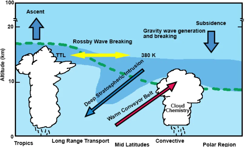
Upper troposphere - lower stratosphere (UTLS)

The upper troposphere-lower stratosphere (UTLS) plays a key role in radiative forcing and

(26)

upper troposphere and the lower stratosphere, from roughly 5 to 22 km in height. The coupling

between dynamics, chemistry, and radiation is found to be strong in the UTLS. The

under-standing of the chemical and dynamical behavior of the tropopause region, and its long-term

variability has become one of the main interests in atmospheric science. The primary

motiva-tion is to understand the coupled processes in UTLS to identify their role in climate change,

which is a necessity for improving weather and climate model simulations of this region

(Wal-lace and Hobbs, 2006).

(27)

The UTLS processes depend crucially on the distribution of greenhouse gases (GHGs),

such as ozone and water vapor, as well as aerosols and clouds. The Fig. 1.2 illustrates some

features of the UTLS region.

Each of the three projects for this thesis provides a means to more accurately measure

temperature and relative humidity in the UTLS, and contributes to our understanding of the

important coupling processes in the UTLS region.

1.2.2 Atmospheric humidity

Water can be found in all three phases in Earth’s atmosphere - solid, liquid, and vapor. The

release of latent heat of water vapor when it condenses into the liquid or solid phase, together

with the Earth’s rotation, drives the large-scale circulation of the atmosphere. Water vapor is

the most dominant greenhouse gas in the Earth’s atmosphere that is highly variable and poorly

understood. Even relatively small changes in the atmospheric water vapor can play a significant

role in the Earth’s atmospheric energy balance (Wallace and Hobbs, 2006).

The amount of the water vapor in the atmosphere can be expressed in many different ways. In this section the various measures of variable atmospheric water vapor content are presented.

Mixing ratio

The mixing ratio is the ratio of mass of the water vapormwv to the mass of the dry airmd in a

certain volume of air and is expressed as

w≡ mwv

md

. (1.1)

The mixing ratio is often expressed in the units of grams of water vapor to kilograms of the dry

(28)

Specific humidity

The specific humidity,qis a measure of the mass of the water vapor with respect to the mass

of air per unit volume defined as,

q= ρwv

ρ , (1.2)

whereρ= ρd+ρwv is the total mass of the air (dry air plus water vapor) per unit volume. The specific humidity is conserved in the absence of mixing or of condensation. In other words,

specific humidity does not vary as the temperature or pressure of an air parcel changes if the

moisture in the air parcel is not removed or added. The stability of the specific humidity makes

it a useful parameter to identify the properties of a moving air mass.

Vapor pressure

The vapor pressure is the partial pressure of the atmospheric water vapor. Vapor pressure can

be expressed as,

e= w

0.622+wP (1.3)

wherePis the total air pressure, assuming water vapor behaves as an ideal gas.

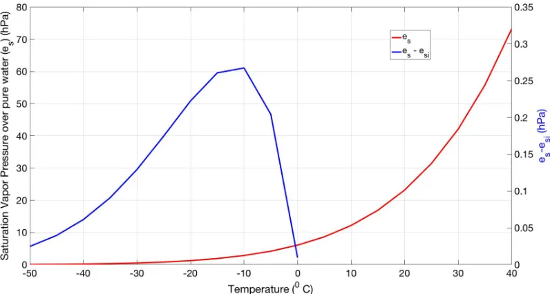
Saturated vapor pressure

The saturation vapor pressure is the partial pressure of the water vapor in equilibrium with

a plane surface of pure water. It solely depends on the temperature. If the temperature is

increased, the molecules will have more internal energy and will vibrate faster. Thus, more

molecules will be able to break free and evaporate from the liquid surface. As a result, the

vapor pressure to increase. For the temperatures below−38◦_{C water will no longer be found}

in the liquid form. Therefore, the saturation will occur over the plane surface of ice instead of

water (Gierens et al., 2000). As the bonds between adjacent molecules are stronger in an ice

surface than they are in a liquid surface, at the same temperature fewer molecules will escape

from an ice surface than from a liquid surface. Therefore, the saturation vapor pressure over

(29)

Figure 1.3: Variation with temperature of the saturation vapor pressureesover a plane surface of pure water (red line) and the difference betweenes and the saturation vapor pressure over a plane surface of icees,i (blue line)(Adapted from Wallace and Hobbs (2006)).

There are several existing formulations that allow the estimation of saturation vapor

pres-sure over both water and ice. For this thesis, I use the saturation vapor prespres-sure equations from

(Hyland, 1983).

The saturation vapor pressure over liquid water (es,w) for temperatures below 0◦ is given

by:

loges,w =

−0.58002206×104

T +0.13914993×10

1₋₀_._48640239_×₁₀−1_×_T

+0.41764768×10−4×T2−0.14452093×10−7×T3

+0.65459673×101×log(T).

(1.4)

The saturation vapor pressure over liquid ice (es,i) for ice is given by (Hyland, 1983):

loges,i =

−0.56745359×104

T +0.63925247×10

1₋₀_._96778430_×₁₀−2_×_T

+0.62215701×10−6×T2+0.20747825×10−8×T3

−0.94840240×10−12×T4+0.41635019×101×log(T).

(30)

Relative humidity

Relative humidity is expressed as a ratio of the vapor pressure to the saturation vapor pressure.

Thus, relative humidity can be estimated over water or ice. The general formulation of the

relative humidity is

RH = e es

×100. (1.6)

whereesis the saturated vapor pressure over water or ice. Relative humidity is the most popular

scale in both meteorology and atmospheric science as it has certain advantages over absolute

measures of water vapor concentration. It is usually in the range of 0% (completely dry) and

100% (saturation) where an absolute scale must be much wider because the concentration of

water molecules decreases from the ground to the tropopause by roughly a factor of 10 000

(Gierens et al., 2012). However, there is nothing to forbid relative humidity from exceeding

100%. Such conditions where the relative humidity exceeds 100% are called supersaturation.

Supersaturation is an unstable state if there is no condensed phase. Another advantage is that

cloud formation is controlled by relative humidity, not by absolute humidity (Gierens et al.,

2012).

Ice supersaturation (ISS)

Ice supersaturation is a frequent atmospheric phenomenon that occurs mainly in the UTLS

region where the temperature reaches below the freezing point. In the upper troposphere,

tem-peratures easily go below −40◦_{C (Gierens et al., 2012). Thus, the super-cooled pure water}

droplets would freeze spontaneously. However, if the water droplets are not pure (contain

aerosol particles, etc.) or are highly diluted they will not freeze spontaneously even at

temper-atures below−40◦C. In order for the droplets to freeze, they need to gain more water molecules from the ambient air. That requires ambient water vapor concentration corresponding to

rela-tive humidity with respect to ice to be more than 145%. Ice formation in these relarela-tively high

supersaturation levels are called ISS. ISS can last for hours or even days and the thickness of

such formations can be from 100 m to 3-4 km. The horizontal extensions of the ISS layers

are not well known yet. ISS is often found within cirrus clouds (ice clouds) and contrails, but

(31)

atmospheric radiation flow (Gierens et al., 2012). However, it was found that as soon as thin

cirrus clouds form within ISS regions, the radiation effects double by two orders of magnitude (Fusina et al., 2007). Thus, ISS plays an important role in cloud formation and as well as in

Earth’s weather and climate.

1.2.3 Instruments and techniques to measure relative humidity

As discussed in the Overview in Section 1.1, measurements from Raman lidars, typically

ground-based, provide an excellent way to obtain vertical temperature and relative humidity

profiles, and I use the Raman lidar technique in this thesis. Details will be discussed in the

fol-lowing sections. In this section I will provide a brief discussion on other humidity measuring

instruments such as radiosondes, microwave radiometers, and weather satellites.

Radiosonde is the most common atmospheric humidity measuring technique and has been

in use since the late 1930s (DuBois, 2002). Radiosondes play an important role in providing

long-term high-quality time series of climatology trends of various parameters. There are about

1,300 radiosonde launch sites all over the globe and most countries share data with the rest of

the world through international agreements. Almost all routine radiosondes are launched 45

minutes before the official observation times of 0000 UTC and 1200 UTC (Seidel et al., 2011). This provides an instantaneous snapshot of the atmosphere. The radiosonde is a small package

consisting of multiple instruments including sensors that measure pressure, temperature, and

relative humidity, and a GPS that returns position information. The radiosonde is suspended

below a large balloon inflated with hydrogen or helium gas and as the balloon rises at about

5 ms−1 _{the radio transmitter sends the measurements obtained by the sensors to the ground}

station. Radiosondes can provide continuous and detailed profiles from the ground to altitudes

of 30 km and above. The hygristor is the relative humidity sensor employed in the radiosondes

located at a place where the outside air passes can reach. A hygristor consists of a glass

slide or plastic strip covered with a moisture sensitive film of lithium chloride (LiCl) and a

binder; metal strips are located along the edges. The electrical resistance of the LiCl changes

with a change in the atmospheric humidity. The hygristor on most radiosondes is designed to

(32)

Hygristors do not provide accurate measurements of relative humidity at temperatures below

the freezing point. When the radiosonde passes through a cloud or a layer of ice, the humidity

sensor can freeze and it will then either not provide any measurements or measure the humidity

inaccurately. To prevent water condensing on the sensors during the ascent of the balloon,

some radiosonde products now occupy two sensor elements that include heating of the of a

sensor elements (Hopkins). However, the radiosonde technique is still not developed enough

to measure relative humidity over ice in regions below freezing. In Chapters 3 and 4 of this

thesis I use the radiosonde measured relative humidity profiles to compare the relative humidity

retrieved from the Raman lidar measurements. For more details of the radiosonde humidity

measurements and their accuracy refer to Miloshevich et al. (2001); Peixoto and Oort (1996);

Sapucci et al. (2005); Bock et al. (2013), and Dirksen et al. (2014).

Weather satellites are outfitted with various types of sensors that can measure atmospheric

water vapor from space (Jones et al., 2009). The operational meteorological observational

sys-tems use nadir sounding (down-looking) instruments to measure the tropospheric water vapor.

Vertical resolution of the nadir microwave humidity sounders is typically several kilometers

and the horizontal resolution is about 10-15 km at nadir. Nadir observations cover

approxi-mately the entire globe (mostly on polar orbits) and the observations are made in both day and

nighttime. Some of the limitations of nadir observations are: limited altitude information from

pressure broadening, only sensitive to region with largest water abundance (troposphere), and

sensitivity to tropospheric clouds (large ice particles or water drops) (Urban, 2013). Satellites

use the limb sounding technique to measure the trace amounts of water vapor in the upper

troposphere and throughout the entire middle atmosphere with resolution of typically only a

few kilometres. The limb observations in the troposphere and lowermost stratosphere are often

limited by the water, cloud, or aerosol absorption depending on wavelength. Further details

of satellite instruments measuring atmospheric water vapour and observation techniques are

available in Urban (2013).

Microwave radiometer is another instrument that is used to measure atmospheric water

vapor. It can be used as a ground-based instrument to measure humidity from the surface

and it can also be used in satellites to measure humidity from space. Microwave radiometers

(33)

Most commercial microwave radiometers operate in the 2060 GHz frequency range, where the

atmospheric thermal emissions are influenced by atmospheric temperature and humidity. A

microwave radiometer consists of an antenna system, microwave radio-frequency components

and a signal processing unit. When appropriate detection frequencies are used, the emission of

microwave radiation from the atmospheric trace gases of liquid water and of ice crystals can

be measured. The emissivity of the substances and their radiative temperature depends on the

substance concentration, pressure, and temperature in the atmosphere. Thus, each substance

can be estimated by measuring its radiative temperature in appropriate frequency bands. The

absorption band of water vapour is located between the frequencies of 20 and 30 GHz. Thus,

measurements of the radiative temperatures in water vapor absorption band allow us to estimate

the integrated water vapour (IWV) content and a profile of absolute humidity. More details of

microwave radiometers are given in L¨ohnert et al. (2009); Hewison (2007), and Liljegren et al.

(2005).

Raman lidars are another potential tool that provides atmospheric humidity measurements

with high spatial and temporal resolution. In this thesis I use the Raman lidar measurements to

retrieve relative humidity and details will be discussed in Section 1.3.

HATPRO Radiometers, dropsondes, and aircraft based instruments are a few other

atmo-spheric humidity measuring techniques. Further details of these instruments and comparisons

of measurements made by each instrument are available in Soden and Lanzante (1996),

Wal-lace and Hobbs (2006), and Buehler et al. (2004).

1.3 Lidars and atmospheric measurements

General description of a lidar

The lidar (light detection and ranging) technique is an active remote sensing technique. It is

one of the tools that has the ability to measure the atmosphere at ambient conditions with high

temporal and spatial resolution, and the potential of covering large altitude ranges in the

atmo-sphere. A typical lidar system (shown in Fig. 1.4) consists of a transmitting system (laser) and a

receiving system (telescope, optical analyzer, etc). Lidars emit light pulses into the atmosphere

(34)

1.3. Lidars and atmospheric measurements 19

that is scattered back is collected by the lidar telescope. Using the lidar’s photon detecting

sys-tem the amount of backscattered light can be measured as a function of altitude. Depending on

the type of interaction processes of the emitted light with the atmospheric constituents, diff er-ent atmospheric parameters and conditions such as temperature, humidity, ozone, particulates,

cloud and wind can be detected (Weitkamp, 2006). To improve the precision of the detection

Figure 1.4: Schematic drawing of lidar system.

the lasers used in the lidars are monochromatic (i.e. one colour /one wavelength), collimated (i.e. very small divergence over large distances), intense (i.e. lots of energy in a small area) and

polarized (i.e. energy is aligned in one direction). There are different types of lidars depending on the laser used and the type of scattering studied. Different types atmospheric scattering are discussed in the next section. The main 5 basic lidar techniques are, elastic-backscatter lidar,

differential absorption lidar (DIAL), Raman lidar, fluorescence lidar, and Doppler lidar. For all three projects in this thesis I am interested in the measurements from Raman lidars and

atmospheric Raman scattering processes.

As shown in Fig. 1.4, the lidar receiving system consists of a telescope that collects all the

backscattered light, an optical analyzer where the signal is spectrally separated, amplified and

(35)

and stored in a computer unit. The diameter of the telescope depends on the purpose of the

lidar and it can vary from 0.1 m to a few meters. The optical analysis of the backscattered light

is often done before the detection. In most cases interference filters are placed in front of the

detector to allow only a certain pass-band around the wavelength of interest enter the detector

(Kovalev and Eichinger, 2004).

Signal detection is typically realized with photomultiplier tubes (PMTs). PMTs are very

sensitive and is used when the backscatter signal is weak ( <10 MHz). PMTs store only the

number of photon counts per time interval after emission of the laser pulse. The efficiency of a PMT to measure and record pulses depends on the time taken up by all components of

the signal processing. The number of photons detected by the PMTs can be measured using

a photon counting system. There are two types of counting systems, nonparalyzable systems

that require a fixed recovery time and paralyzable systems that don’t. The fixed recovery time

of a counting system is called the dead time of the system. In a paralyzable system if the

time gap between two signals reaching the detector is larger than dead time then the event

will be recorded. Thus, the observed rate is equal to the rate at which time intervals occur

that exceed dead time. The main difference between the two types of counting systems is that nonparalyzable detector systems are not effected if the signal is not processed whereas paralyzable detector systems are effected (Wandinger, 2005a).

In lidars for strong backscatter signals typically the measurements in lower altitudes are

recorded using analog recorders where the average current produced by the photo pulses is

measured. Then analog-to-digital signal conversion and digital signal processing need to be

performed (Wandinger, 2005a).

Atmospheric scattering related to lidar

Atmospheric scattering is the redirection of the original path of electromagnetic (EM) radiation

(i.e. an incident light ray) traveling through the atmosphere due to particles or gas molecules

present in the atmosphere. As the EM wave interacts with the atmospheric particles or gas

molecules the electron’s cloud within the atmospheric constituent starts to oscillate periodically

with the same frequency as the incident EM wave. This oscillation later induces a dipole

(36)

of EM radiation, thereby resulting in scattered light. The atmospheric scattering depends on

the wavelength of the incident radiation and also on the size of the atmospheric constituent that

scatters the radiation. In this section, I will briefly discuss three main atmospheric scattering

processes: Mie scattering, Rayleigh scattering, and Raman scattering.

Rayleigh scattering is the most dominant scattering mechanism in the upper atmosphere

and it is a type of an elastic scattering, meaning Rayleigh scattered radiation has the same

frequency as the incident radiation. Rayleigh scattering occurs when particles are very small

compared to the wavelength of the radiation. These could be particles such as small specks of

dust or nitrogen and oxygen molecules (Kovalev and Eichinger, 2004).

The intensity of Rayleigh scattering varies inversely with the fourth power of the

wave-length (λ−4). Rayleigh scattering is the phenomenon behind the sky appearing blue during the

day and red/orange during sunrise and sunset. As sunlight travels through the atmosphere, the shorter wavelengths (i.e. blue) of the visible spectrum scatter more than the longer

wave-lengths. At sunrise and sunset, the light has to travel farther through the atmosphere than

daytime. Hence, the scattering of the shorter wavelengths is more complete and this allows a

greater proportion of the longer wavelengths of the visible spectrum to penetrate through the

atmosphere (Kovalev and Eichinger, 2004).

For the atmosphere, assuming that the scattering is from a spherically symmetric molecule

the total Rayleigh scattering cross-section can be approximated (Kovalev and Eichinger, 2004):

σ' 32π

3

3λ4

n−1

N

!2

(1.7)

whereNis the number density of the molecules andnis the refractive index.

When using Rayleigh scattering for diagnostics usually the scattered light is collected over

a limited solid angle. Therefore, it is useful to define a differential cross-section for Rayleigh scattering such that

∂σ ∂Ω '

4π2

λ4

n−1

N

!2

sin2φ, (1.8)

whereφis the scattering angle andΩis the solid angle (Kovalev and Eichinger, 2004).

Mie scattering is an elastic scattering that occurs due to the particles that are about the

(37)

vapor molecules, and other large atmospheric molecules cause Mie scattering. The Mie

sig-nal is proportiosig-nal to the square of the particle diameter and is much stronger than Rayleigh

scattering.

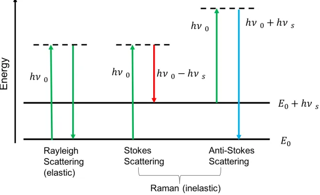
Raman scattering is an inelastic process where monochromatic light or photons is scattered

offa molecule at a different wavelength than the incident. Thus, the scattered photons energy will be different than the incident photon. The change in energy is proportional to the rotational or vibrational energy levels of the atom or the molecule that the photon scattered off(Kovalev and Eichinger, 2004). As shown in Fig. 1.5, the scattered photon can either gain energy from

Figure 1.5: The different types of light scattering: Rayleigh scattering (no exchange of en-ergy: incident and scattered photons have the same energy), Stokes Raman scattering (atom or molecule absorbs energy: scattered photon has less energy than the incident photon) and anti-Stokes Raman scattering (atom or molecule loses energy: scattered photon has more energy than the incident photon).

the interaction and shift to a higher frequency (red-shift) or lose energy from the interaction and

shift to a lower frequency (blue-shift). The processes of gaining and losing energy are known

as Stokes and anti-Stokes shift respectively. The frequency shift for the scattering molecules is

given by,

∆v˜= v˜i−v˜s=

∆E

hc (1.9)

(38)

between the molecular energy levels involved,his the Planck’s constant, andcis the speed of

light in a vacuum.

Figure 1.6: Raman backscatter spectrum of the atmosphere for an incident laser wavelength of 355 nm, normal pressure, a temperature of 300 K, an N2 and O2 content of 0.781 and 0.209, respectively, and a water-vapor mixing ratio of 10 g/kg. The curves for liquid water and ice are arbitrarily scaled. (Figure 9.2 in Wandinger (2005b))

Since the scattering targets of interest are mostly diatomic molecules in the atmosphere such

as nitrogen and oxygen, I expect that there will be an energy shift due to both the vibrational and

rotational transitions as shown in Fig. 1.6. The vibrational energy transition levels for diatomic

molecules can be approximated using the model of a freely rotating harmonic oscillator:

Evib,v =hc0vvib(˜ v+1/2), for v=0,1,2, .... (1.10)

where vvib is the specific vibrational wave-number of the molecule and v is the vibrational

quantum number (Behrendt, 2005). For the energy levels for the rotational quantum numbers

is approximated by,