Parallel Patient Treatment Time Prediction Algorithm For in Queuing
Management by Big Data
K.Lavanya & B.Rama Ganesh
(M.Tech), Department of CSE, VEMU INSTITUTE OF TECHNOLOGY, Chittoor.
Asst.Prof,M.tech,(Ph.D) , Department of CSE, VEMU INSTITUTE OF TECHNOLOGY, Chittoor.
ABSTRACT: Successful patient line administration to limit
tolerant hold up deferrals and patient overcrowdings one of the real difficulties confronted by healing facilities. Pointless and irritating sits tight for long stretches result in considerable human asset and time wastage and increment the disappointment continued by patients. For every patient in the line, the aggregate treatment time of the considerable number of patients before him is the time that he should hold up. It would be advantageous and best if the patients could get the most proficient treatment plan and know the anticipated holding up time through a versatile application that updates progressively. Along these lines, we propose a Patient Treatment Time Prediction (PTTP) calculation to foresee the sitting tight time for every treatment undertaking for a patient. We utilize reasonable patient information from different clinics to acquire a patient treatment time demonstrate for each undertaking. In view of this extensive scale, sensible dataset, the treatment time for every patient in the present line of each errand is anticipated. In view of the anticipated holding up time, a Hospital Queuing-Recommendation (HQR) framework is created. HQR ascertains and predicts a proficient and helpful treatment arrange suggested for the patient. As a result of the huge scale, practical dataset and the necessity for constant reaction, the PTTP calculation and HQR framework order effectiveness and low-idleness reaction. We utilize an Apache Spark-based cloud execution at the National Supercomputing Center in Changsha to accomplish the previously mentioned objectives. Broad experimentation and reenactment comes about show the viability and relevance of our proposed model to suggest a successful treatment get ready for patients to limit their hold up times in healing centers.
INDEX TERMS: Apache spark, big data, cloud computing, hospital queuing recommendation, patient, treatment time prediction.
I.INTRODUCTION
In this paper, we propose a PTTP calculation and a HQR framework. Considering the continuous prerequisites, gigantic information, and multifaceted nature of the framework, we utilize huge information and distributed computing models for effectiveness and adaptability. The PTTP calculation is prepared in light of an enhanced Random Forest (RF) calculation for every treatment errand, and the holding up time of each assignment is anticipated in view of the prepared PTTP display. At that point, HQR prescribes an effective and advantageous treatment get ready for every patient. Patients can see the suggested arrange and anticipated holding up time progressively utilizing a versatile application. Broad experimentation and application comes about demonstrate that the PTTP calculation accomplishes high
exactness and execution. Our commitments in this paper can be outlined as takes after. A PTTP calculation is proposed in light of an enhanced Random Forest (RF) calculation. The anticipated holding up time of every treatment errand is gotten by the PTTP show, which is the total of all patients' likely treatment times in the current queue.An HQR framework, is proposed in view of the anticipated holding up time. A treatment suggestion with an efcient and advantageous treatment arrange and the minimum sitting tight time is prescribed for every patient.
The PTTP calculation and HQR framework are parallelized on the Apache Spark cloud stage at the National Supercomputing Center in Changsha (NSCC) to accomplish the previously mentioned objectives. Broad doctor's facility information are put away in the Apache HBase, and a parallel arrangement is utilized with the Map Reduce and Resilient Distributed Datasets (RDD) programming model. The rest of the paper is sorted out as takes after. Area 2 surveys related work. Segment 3 points of interest a PTTP calculation and a HQR framework. The parallel execution of the PTTP calculation and HQR framework on the Apache Spark cloud condition is point by point in Section 4. Test results and assessments are introduced in Section 5 as for the suggestion precision and execution. At long last, Section 6 finishes up the paper with future work and headings. To enhance the precision of the information investigation with nonstop components, different improvement techniques for characterization and relapse calculations are proposed. A self-versatile acceptance calculation for the incremental development of paired relapse trees was introduced in [1]. Tyree et al. [2] presented a parallel helped relapse tree calculation for web seek positioning. In [3], a multi-branch choice tree calculation was proposed in light of a relationship part foundation. Other enhanced order and relapse tree techniques were proposed in [4] [6].
treatment undertaking, we utilize the irregular timberland calculation to prepare the patient treatment time utilization in view of both patient and time qualities and afterward assemble the PTTP demonstrate. Since patient treatment time utilization is a nonstop factor, a Classication and Regression Tree (CART) model is utilized as a meta-more tasteful in the RF calculation. As a result of the weaknesses of the first RF calculation and the qualities of the patient information, in this paper, the RF calculation is enhanced in 4 perspectives to get a compelling outcome from expansive scale, high dimensional, consistent, and uproarious patient information. Contrasted and the first RF calculation, our PTTP calculation in view of an enhanced RF calculation has sign cannot focal points as far as exactness and execution. In addition, there is no current research on doctor's facility lining administration and proposals. Consequently, we propose a HQR framework in light of the PTTP display. To the best of our insight, this paper is the rst endeavor to tackle the issue of patient sitting tight time for healing center lining administration registering. A treatment lining suggestion with an effective and advantageous treatment arranges and the slightest sitting tight time is prescribed for every patient.
II. PATIENT TREATMENT TIME PREDICTION ALGORITHM
To build the PTTP model based on patient and time characteristics, a PTTP algorithm is proposed. The PTTP model is based on an improved RF algorithm and is trained from the massive, complex, and noisy hospital treatment data.
A. PROBLEM DEFINITION AND DATA PREPROCESSING
1) PROBLEM DEFINITION
Prediction based on analysis and processing of massive noisy patient data from various hospitals is a challenging task. Some of the major challenges are the following:
(1) Most of the data in hospitals are massive, unstructured, and high dimensional. Hospitals produce a huge amount of business data every day that contain a great deal of information, such as patient information, medical activity information, time, treatment department, and detailed information of the treatment task. Moreover, because of the manual operation and various unexpected events during treatments, a large amount of incomplete or inconsistent data appears, such as a lack of patient gender and age data, time inconsistencies caused by the time zone settings of medical machines from different manufacturers, and treatment records with only a start time but no end time. The time consumption of the treatment tasks in each department might not lie in the same range, which can vary according to the content of tasks and various circumstances, different periods, and different conditions of patients. For example, in the case of a CT scan task, the time required for an old man is generally longer than that required for a young man. There are strict time requirements for hospital queuing management and recommendation. The speed of executing the PTTP model and HQR scheme is also critical.
DATA PREPROCESSING
In the preprocessing phase, hospital treatment data from different treatment tasks are gathered. Substantial numbers of patients visit each hospital every day. Let S be a set of patients in a hospital, and a patient who has been registered and his information is represented by si. Assume that there are N patients in S:
where each patient si can have speci c unchanged parameters, e.g.,
name, ID, gender, age, and address. Some of these parameters are useful to our analysis, whereas others are not. Each patient can visit multiple treatment tasks according to his health condition. Let
Xjsi be a set of treatment tasks for patient si during a speci c visit:
where each treatment task record xi can consist of multiple
information Y , e.g., task name, task location, department, start time, end time, doctor, and attending staff:
whereyj is a feature variable of the record of treatment task xi.
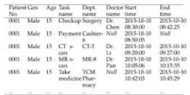
Here, for a single visit, we have a single record for patient name, age, gender, and multiple records for treatment tasks, as shown in Table 1.
TABLE 1.
Example of treatment records.
The work ow of the preprocessing task can be depicted by the following steps.
a: GATHER DATA FROM DIFFERENT TREATMENT TASKS
Depending on statistics, the number of patients in a medium-sized hospital lies between 8,000 and 12,000 per day, and the number of remedial treatment data records is between 120,000 and 200,000. These data are gathered from different
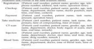
TABLE 2.
treatment tasks, including registration, medical examination, inspection, drug delivery, payment, and other related tasks. The formats of the data for different treatment tasks are shown in Table 2.
b: CHOOSE THE SAME DIMENSIONS OF THE DATA
The hospital treatment data generated from different treatment tasks have different contents and formats as well as varying dimensions. To train the patient time consumption model for each treatment task, we choose the same features of these data, such as the patient information (patient card number, gender, age, etc.), the treatment task information (task name, department name, doctor name, etc.), and the time information (start time and end time). Other feature subspaces of the treatment data are not chosen because they are not useful for the PTTP algorithm, such as patient name, telephone number, and address.
c: CALCULATE NEW FEATURE VARIABLES OF THE DATA
To train the PTTP model, various important features of the data should be calculated, such as the patient time consumption of each treatment record, day of week for the treatment time, and the time range of treatment time. For example, in the treatment record of the CT scan task in Table 1, the start time is ``2015-10-10 09:20:00'' and the end time is ``2015-10-10 09:27:00'', the time consumption for this patient in the treatment is ``420 (s)'', the day of the week is ``Saturday'', and the time range is ``09''.
III . PARALLEL IMPLEMENTATION OF THE PTTP ALGORITHM AND HQR SYSTEM
Massive historical treatment data (comprise more than 5 TB, and increase every day) are initially stored in H Base. Then, the PTTP model and HQR system are parallelized in the Apache Spark cloud platform. Thus, the performance of the algorithms is improved signicantly.
A. PARALLEL IMPLEMENTATION OF THE PTTP MODEL
We parallelize the PTTP model on the Spark cloud platform. A dual parallelization training process is performed. The k training subsets are trained in a parallel process, and k CART regression trees are built at the same time. Then, the M variables in the training subsets are calculated in parallel in the node-splitting process of each tree. The parallel training process of the PTTP model is implemented in the Spark computing cluster with the RDD programming model. Distinct from the MapReduce model on the Hadoop platform, the intermediate results generated in the training process of the PTTP model are stored in the memory system on the Spark platform as RDD objects. Before the training
process, the treatment data are loaded from HBase to the Spark Tachyon memory system as an RDD object. An RDD object
RDDoriginal is de ned to save the training dataset. Then, k training
subsets are sampled as K RDD objects from RDDoriginal ; each of
them is de ned as RDDtraini. Other k RDD objects are created to
save relatedOOB subsets; each of them is defined as RDDOOBi. The
K training subsets are allocated to k map tasks at the same time and are allocated to multiple slave nodes. Then, these training subsets are calculated in parallel with the RDD programming model including a series of operations. Finally, k regression tree models are obtained.
The dual parallelization training process of the PTTP model is shown in Fig. 1.
In the RDD programming model, each RDD object supports two types of operations, i.e., transformation and action. Transformation operations include a series of operations on an RDD object, such as map, lter, atMap, map Partitions, union, and
join. Then, a new RDD object is returned from each transformation operation. Action operations include a series of operations on an RDD object, such as reduce, collect, count, save As Hadoop File, and count Bykey, that compute a resul and callback to the driver program or save it to an external storage system. The detailed steps of the dual parallelization training process of the PTTP model are presented in Algorithm 3. The training processes of each training subset RDDtraini and the OOB subset RDDOOBi comprise the
following stages.
FIGURE 1.Dual parallelization training process of the PTTP
model.
In stage 1, there are build Feature Data and ndSplits Feature functions, which perform a transformation operation and an action operation, respectively. In the build FeatureData
function, feature subspaces of RDDtraini are mapped to a new RDD
object with M partitions, which refer to the M feature variables. The loss function of each feature variable subspace and each potential split point value of the variable are calculated. In the
function are sorted, and the feature variable with the least value is selected as the rst node of CART tree Ti, which is created as RDD
object RDDTi.
FIGURE 2.Parallelization recommendation process of the HQR
system.
In stage 2, there are two split functions and a nd Best Splits function. In the rstsplit function, the training subset RDDtraini
is split into two forks by a split point in the current feature subspace, which is shown as RDDL=Rtree in Fig. 2. For each branch,
there is and Best Splits function. In the nd BestSplits function, the same feature variables continue to be selected, and the results of sets of the potential splitting values for the current feature subspace are calculated.
B. PARALLEL IMPLEMENTATION OF THE HQR SYSTEM
Usually, there are a number of treatment tasks for each patient, and many patients waiting in the queue of each treatment task. Therefore, a parallel HQR system is implemented for each patient if there is more than one treatment task for the patients. The process of the parallel HQR system is shown in Fig. 2.
Assume that there are n treatment tasks for the current patient to complete and that there is a number of patients waiting in the queue of each treatment task. In the parallelization solution, n
RDD objects are created to refer to the n treatment tasks. There is a number of partitions in each RDD object that refer to patients waiting in the queue of each task. Let partition Uij be the jth patient
waiting for the ith treatment task.
Step 1: For each patient Uij in a task Taski, the time consumption of
the patient might generate in the ith task, as predicted by the trained PTTP model. In this step, the time consumption for each patient Uij is calculated with the k trained CART trees of the
RF-based PTTP model in ashuf e function, and the predicted patient treatment time consumption Tij is derived.
Step 2: The patient treatment time consumption of all ofthe patients in each task is added in a sum function, and the predicted waiting time Ti of each task is obtained. An RDD object (Taski; Ti)
is created for each task.
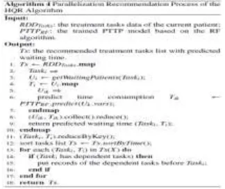
Step 3: The predicted waiting times for all of the tasks for the current patient are sorted in ascending order with a sort function. A new RDD object Ts is created to save the sorted waiting times of all of the treatment tasks. Hence, the parallel hospital queuing recommendation schema for the current patient is performed. The detailed steps of the parallel HQR algorithm are presented in Algorithm 4.
IV. EXPERIMENTS AND APPLICATIONS & RESULT ANALYSIS
In this section, the accuracy and performance of the proposed algorithm are evaluated through a series of experiments. The algorithm is applied to an actual hospital project in China. Section 5.1 presents the experimental settings.
The experiment result analysis of the PTTP algorithm and the HQR system are presented in Section 5.2, Section 5.3 presents the accuracy and robustness evaluation, and performance evaluation is provided in Section 5.4.
A. EXPERIMENT AND APPLICATION SETUP
The HQR system consists of two main modules: a decision maker and recommendation module and a mobile application interface module. In the decision maker and recommendation module, treatment data are transmitted to the HBase database in NSCC from hospitals regularly. The system and experiments are performed on a Spark cloud platform, which is constructed at the National Supercomputing Center in Changsha to achieve the aforementioned goals. Each computing node runs Linux operating system Ubuntu 12.04.4, with 2 Intel Xeon Westmere EP CPUs, 6 cores, 2.93GHZ, and 48GB memory. All of the nodes are connected by a high-speed Gigabit network and are con gured with Hadoop 2.6.0 and Spark 1.6.0. The algorithm is implemented in Java 1.7.0 and Scala 2.11.7. In our experiments, datasets covering three years (2012 - 2014) are chosen from an actual hospital application, as shown in Table 5.
TABLE 5.
In Table 5, the departments of the hospital include the nancial room, the Emergency Department (ED), CT scan, MR scan, B-model ultrasound, color Doppler ultrasound, nuclear medicine, and the pharmacy. There are various treatment tasks in each department. We analyze the patient treatment time consumption of the CT scan task with time factors and patient characteristics. Because of the content of the activities and various circumstances, the patient treatment time consumption of treatment tasks in each department can vary. At the same time, the time consumption in the same department might be different due to the different treatment tasks, different periods, and different conditions of patients.
1) TREATMENT TIME CONSUMPTION WITH TIME FACTORS
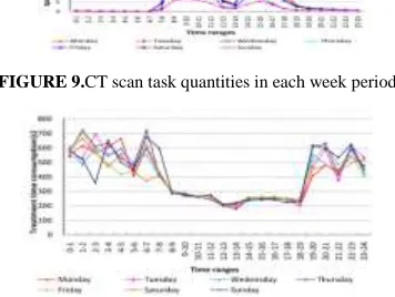
The CT scan treatment task quantities are depicted in Fig. 9. As seen in Fig. 9, there are two peaks of the CT scan task every day. The rst peak comes from 8 am to 11 am, and the second peak comes from 2 pm to 5 pm. The nadir point of each day is in the range of 0 am -7 am in the morning, 12 pm to 1 pm at noon, and 6 pm to 11 pm in the evening. The overall number of patients per weekend day is less than that on individual weekdays.
After the training process of the PTTP algorithm, the time consumptions of all of the treatment tasks in the experiment are trained. The time consumption of CT scan task with time factors (part) is shown in Fig. 10.
FIGURE 9.CT scan task quantities in each week period.
FIGURE 10. Treatment time consumption of the CT scan task
with time factors (part).
Each point in Fig. 10 refers to a value of one leaf node in the regression trees of the PTTP model. Consider 9 am on a weekday for a CT scan task to be an example of a peak time scenario; the average output of a CT scan operation is approximately 40 every day. There are 43,200 records at the leaf nodes of the CART tree model. The time consumption is close to 240 s (approximately 4.0 min) for a CT scan task. Conversely, at the nadir point, there are 0 or 1 CT scan tasks in each hour. There are 0 - 1095 (1 365 days 3 years) records at the leaf node of the tree model. Obviously, because there are approximately 43,200 (40 365 days 3 years) records at the leaf node for peak time case, the value of trained
treatment time consumption is smooth and steady. At the nadir point, the value of trained treatment time consumption is undulate because of the small number of training samples. Consequently, having fewer records in each leaf node of the tree model results in less accuracy.
2) TREATMENT TIME CONSUMPTION WITH PATIENT CHARACTERISTICS
The treatment time consumption of a CT scan task with patient characteristics (part) is shown in Fig. 11.
FIGURE 11.Treatment time consumption of the CT scan task with
patient characteristics (part).
As seen in Fig. 11, for patients with ages ranging from 20 to 40, time consumption of each CT scan task is approximately 245 s (approximately 4.1 min) for both men and women. As age increases, the time required for each patient's CT scan task increases. For example, the time consumption for a male patient at age 90 is approximately 786 s (approximately 13.1 min). At the same time, generally speaking, the time consumption for a female patient is greater than that for a male in the same age range.
3) HQR SYSTEM IN A MOBILE APPLICATION
FIGURE 12.Mobile interfaces of the HQR system. (a)
Recommended tasks list. (b) Details of the waiting queue.
The predicted waiting time of all of the treatment tasks is calculated by the PTTP model. Then, a treatment recommendation with the least waiting time is advised. Fig. 12(a) shows that there are 10 people waiting for the CT scan before the current patient (including the people waiting in the queue and in processing), and the predicted waiting time is 26.0 min. Fig. 12(b) shows the details of the waiting queue for the CT scan. The total predicted time consumption of 10 people is 78.0 min, and there are 3 machines available in parallel. Therefore, the predicted waiting time of the current patient is 26.0 min. Moreover, the status of the waiting queue is updated in real-time. The experimental results show that the HQR system provides a recommendation with an effective treatment plan for patients to minimize their wait times in hospitals.
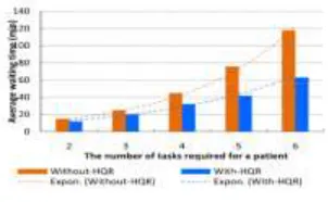
4) AVERAGE WAITING TIME FOR PATIENTS
FIGURE 13.Average waiting time for patients.
To evaluate the efciency of our HQR system, various experiments about average waiting time for patients in the with-HQR case with that in the without-HQR case are performed. Each case is under the treatment data with 5000 patients and 20,000 treatment records. We accounted and compared the average waiting time of patients in the with-HQR case with that in the without-HQR case. The results of comparison are presented in Fig. 13.
C. ACCURACY AND ROBUSTNESS ANALYSIS
To evaluate the accuracy and robustness of our improved-RF-based PTTP algorithm, we implemented the PTTP algorithm improved-RF-based on the original random forest (refereed as PTTP-ORF). The accuracies of the PTTP algorithm and PTTP-ORF algorithm are analyzed under different ratios of noisy data.
1) RESULTS EVALUATION OF NOISE REMOVAL
TABLE 6.
Specific conditions of six leaf nodes in the experiments.
In Section 3.2.2, a noise removal method is introduced in the training process of the regression tree model. The effect of noise removal is validated and analyzed. Six groups of leaf node data in the regression tree models are discussed in experiments, the speci c conditions of the six groups of leaf nodes are shown in Table 6.
The results of noise removal for the PTTP algorithm are presented in Fig. 14.
FIGURE 14.Noisy data removal results for the PTTP algorithm.
Fig. 14(a) is a box plot of a leaf node with the condition of ``CT-1''. The patient treatment time consumption in this case is between 0 and 2500 s (approximately 0.0 - 41.6 min). The boundaries of the box plot in this case are 0 and 480 s (approximately 8.0 min), and the median value is 240 s (approximately 4.0 min). That is, most of the patient treatment time consumption data are in this range, which is understandable for people in the 25-45 age range in the treatment operation of a CT scan task. In Fig. 14(b), time consumption is in the range 0 - 8000 s (approximately 0.0 - 133.3 min) for male aged 65 - 85 in the CT scan task. After noise removal, the time range is changed to 0 - 1995; the median value is 710 s (approximately 11.8 min). In Fig. 14(c), the time consumption range is 0 - 1740 s (approximately 0.0 - 29.0 min) after noise removal, rather than the range of 0 - 2500 s. The median value is 720 s (approximately 12.0 min) for one treatment of the MR scan task. Two examples of noisy data removal from patient treatment time consumption are shown in Fig. 15.
FIGURE 15.Examples of noisy data removal from patient
treatment time consumption.
Summarizing, after noise removal, the value ranges of patient treatment time consumption obviously decrease.
FIGURE 16.Accuracy of different algorithms with different tree
scales.
2) ALGORITHM ACCURACY ANALYSIS WITH DIFFERENT TREE SCALES
To illustrate the accuracy of the PTTP algorithm, various experiments are performed on the dataset shown in Table 5. Each case is under different scales of the decision tree. By counting the average accuracies of the algorithms, the different accuracies of various environments are compared and analyzed. The results are presented in Fig. 16. Fig. 16 shows that the average accuracy of the PTTP algorithm based on different improved random forest algorithms is not high when the number of regression trees in each algorithm is equal to 10. With an increase in the number of decision trees, the average accuracy increases gradually and tends toward a convergence condition. The accuracy of the PTTP algorithm is greater than that of PTTP-ORF by 3.72% on average and 5.10% in the best case, when the number of decision trees is equal to 200. Consequently, compared with PTTP-ORF, the PTTP algorithm, which has been optimized in four aspects, can signicantly increase the accuracy.
3) ALGORITHM ACCURACY ANALYSIS UNDER DIFFERENT NOISE RATIOS
FIGURE 17.Accuracy of different algorithms under different
noise ratios.
To demonstrate the accuracy of our algorithm, we conduct experiments with algorithms, such as the PTTP and PTTP-ORF. We construct the noisy data by modifying the values of the original data randomly according to different noise ratio requirements. The scales of the noise ratios are located in the range of {1%, 4%, 8%, 12%, 16%, 20%, 24%, 28%, 32%, 36%, 40%}. The number of training samples in the cases is 100,000, and the number of regression trees in the random forest model is 500. The result of comparative analysis is presented in Fig. 17.
Fig. 17 states that in each case, when the proportion of noisy data increases, the average accuracy of PTTP-ORF decreases quickly. When the scale of noisy data increases from 1% to 40%, the accuracy of PTTP-ORF decreases from 88.70% to 74.50%. Therefore, noisy data have a sign cant degree of in uence on PTTP-ORF. Accuracy of PTTP-ORF is in uenced by a large volume of noisy data. In addition, as the proportion of noisy data increases, the tendency of the accuracy of our PTTP algorithm decrease is steady. When the proportion of noisy data increases from 1% to 50%, the average accuracy of PTTP decreases from 91.90% to 82.60%.Obviously, the average accuracy of PTTP is greater than that of the other two algorithms under each condition of noise ratio. Consequently, the PTTP algorithm can reduce the in uence of noisy data effectively and achieve good robustness.
D. PERFORMANCE EVALUATION
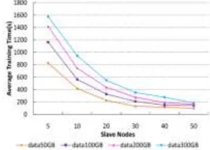
1) PERFORMANCE EVALUATION OF THE PTTP ALGORITHM
To evaluate the performance of the PTTP algorithm, four groups of historical hospital treatment data are trained at different scales of the Spark cluster. The sizes of these datasets are 50GB, 100GB, 300GB, and 200GB. The scale of slave nodes of the Spark cluster in each case increases from 5 to 80. By observing the average execution time of the PTTP algorithm in each case, different performances across various cases are compared and analyzed. The results are presented in Fig. 18.
From Fig. 18, the advantage of the parallel algorithm in cases of large-scale data is greater than in cases of small-scale data. The benefit is more obvious when the number of slave nodes increases. As the number of cluster nodes increases from 5 to 80, the average execution time of the PTTP model decreases from 879 to 285 s for 300GB of data, and decreases from 328 to 81 s for 50GB of data.
FIGURE 18.Performance evaluation of the PTTP algorithm.
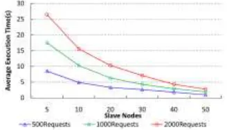
2) PERFORMANCE EVALUATION OF THE HQR SYSTEM
2000. In the case of 80 nodes in the Spark cluster, the average execution time of HQR is 0.9 s for 500 requirements, 1.9 s for 1000, and 2.7 s for 2000. As the number of cluster nodes increases from 5 to 80, the average execution times of the HQR system in the three groups decrease at the ratios of 8.85, 9.21 and 9.63 times. The actual operational results of the algorithm are close to the theoretical results.
FIGURE 19.Performance evaluation of the HQR system.
V. CONCLUSION
In this paper, a PTTP algorithm based on big data and the Apache Spark cloud environment is proposed. A random forest optimization algorithm is performed for the PTTP model. The queue waiting time of each treatment task is predicted based on the trained PTTP model. A parallel HQR system is developed, and an efficient and convenient treatment plan is recommended for each patient. Extensive experiments and application results show that our PTTP algorithm and HQR system achieve high precision and performance. Hospitals' data volumes are increasing every day. The workload of training the historical data in each set of hospital guide recommendations is expected to be very high, but it need not be. Consequently, an incremental PTTP algorithm based on streaming data and a more convenient recommendation with minimized path-awareness are suggested for future work.
REFERENCES
[1] R. Fidalgo-Merino and M. Nunez, ``Self-adaptive induction of regression trees,'' IEEE Trans. Pattern Anal. Mach. Intell., vol. 33, no. 8, pp. 1659 1672, Aug. 2011.
[2] S. Tyree, K. Q. Weinberger, K. Agrawal, and J. Paykin, ``Parallel boosted regression trees for Web search ranking,'' in
Proc. 20th Int. Conf. WorldWide Web (WWW), 2012, pp. 387 396.
[3] N. Salehi-Moghaddami, H. S. Yazdi, and H. Poostchi, ``Correlation based splitting criterionin multi branch decision tree,''
Central Eur. J. Comput.Sci., vol. 1, no. 2, pp. 205 220, Jun. 2011.
[4] G. Chrysos, P. Dagritzikos, I. Papaefstathiou, and A. Dollas, ``HC-CART: A parallel system implementation of data mining classication and regression tree (CART) algorithm on a multi-FPGA system,'' ACM Trans.Archit. Code Optim., vol. 9, no. 4, pp. 47:1 47:25, Jan. 2013.
[5] N. T. Van Uyen and T. C. Chung, ``A new framework for distributed boosting algorithm,'' in Proc. Future Generat. Commun. Netw. (FGCN), Dec. 2007, pp. 420 423.
[6] Y. Ben-Haim and E. Tom-Tov, ``A streaming parallel decision tree algorithm,'' J. Mach. Learn. Res., vol. 11, no. 1, pp. 849 872, Oct. 2010.
[7] L. Breiman, ``Random forests,'' Mach. Learn., vol. 45, no. 1, pp. 5 32, Oct. 2001.
[8] G. Yu, N. A. Goussies, J. Yuan, and Z. Liu, ``Fast action detection via discriminative random forest voting and top-K subvolume search,'' IEEETrans. Multimedia, vol. 13, no. 3, pp. 507 517, Jun. 2011.
[9] C. Lindner, P. A. Bromiley, M. C. Ionita, and T. F. Cootes, ``Robust and accurate shape model matching using random forest regression-voting,'' IEEE Trans. Pattern Anal. Mach. Intell., vol. 37, no. 9, pp. 1862 1874,Sep. 2015.
[10] K. Singh, S. C. Guntuku, A. Thakur, and C. Hota, ``Big data analytics framework for peer-to-peer botnet detection using random forests,'' Inf.Sci., vol. 278, pp. 488 497, Sep. 2014. [11] S. Bernard, S. Adam, and L. Heutte, ``Dynamic random forests,'' PatternRecognit. Lett., vol. 33, no. 12, pp. 1580 1586, Sep. 2012.
[12] H. B. Li, W. Wang, H. W. Ding, and J. Dong, ``Trees weighting random forest method for classifying high-dimensional noisy data,'' in Proc. IEEE7th Int. Conf. e-Business Eng. (ICEBE), Nov. 2010, pp. 160 163.
[13] G. Biau, ``Analysis of a random forests model,'' J. Mach. Learn. Res., vol. 13, no. 1, pp. 1063 1095, Apr. 2012. [14] S. Meng, W. Dou, X. Zhang, and J. Chen, ``KASR: A keyword-aware service recommendation method on MapReduce for big data applications,'' IEEE Trans. Parallel Distrib. Syst., vol. 25, no. 12, pp. 3221 3231,Dec. 2014.
[15] Y.-Y. Chen, A.-J. Cheng, and W. H. Hsu, ``Travel recommendation by mining people attributes and travel group types from community-contributed photos,'' IEEE Trans. Multimedia, vol. 15, no. 6, pp. 1283 1295, Oct. 2013.
[16] X. Yang, Y. Guo, and Y. Liu, ``Bayesian-inference-based recommendation in online social networks,'' IEEE Trans. Parallel Distrib. Syst., vol. 24, no. 4, pp. 642 651, Apr. 2013. [17] G. Adomavicius and Y. Kwon, ``New recommendation techniques for multicriteria rating systems,'' IEEE Intell. Syst., vol. 22, no. 3, pp. 48 55, May/Jun. 2007.
[18] G. Adomavicius and A. Tuzhilin, ``Toward the next generation of recommender systems: A survey of the state-of-the-art and possible extensions,'' IEEE Trans. Knowl. Data Eng., vol. 17, no. 6, pp. 734 749, Jun. 2005.
[19] X. Wu, X. Zhu, G.-Q. Wu, and W. Ding, ``Data mining with big data,'' IEEE Trans. Knowl. Data Eng., vol. 26, no. 1, pp. 97 107, Jan. 2014.
[20] Apache. (Jan. 2015). Hadoop. [Online]. Available: http://hadoop. apache.org
[21] Apache. (Jan. 2015). Spark. [Online]. Available: http://spark-project.org
[22] J. Dean and S. Ghemawat, ``MapReduce: Simplied data processing on large clusters,'' Commun. ACM, vol. 51, no. 1, pp. 107 113, Jan. 2008.
[23] M. Zahariaet al., ``Resilient distributed datasets: A fault-tolerant abstraction for in-memory cluster computing,'' in
[24] Apache. (Jan. 2015). Mahout.[Online]. Available: http://mahout. apache.org
[25] Y. Xu, K. Li, L. He, L. Zhang, and K. Li, ``A hybrid chemical reaction optimization scheme for task scheduling on heterogeneous computing systems,'' IEEE Trans. Parallel Distrib. Syst., vol. 26, no. 12, pp. 3208 3222, Dec. 2015.
[26] K. Li, X. Tang, B. Veeravalli, and K. Li, ``Scheduling precedence constrained stochastic tasks on heterogeneous cluster systems,'' IEEE Trans. Comput., vol. 64, no. 1, pp. 191 204, Jan. 2015.
[27] D. Dahiphale et al., ``An advanced MapReduce: Cloud MapReduce, enhancements and applications,'' IEEE Trans. Netw. Service Manage., vol. 11, no. 1, pp. 101 115, Mar. 2014.
[28] M. Zaharia et al., ``Fast and interactive analytics over hadoop data with spark,'' in Proc. USENIX NSDI, 2012, pp. 45 51.
B.Rama Ganesh is presently
working as Professor,Vemu
Institute of Technology,Tirupati in Andhra Pradesh. B.Rama Ganesh
completed his B.Tech,M.Tech
from JNTU - Hyderabad, Ph.D pursuing in CSE from GITAM
Univesity.i have 12 Years
experience in teaching.
Ms.K.Lavanya has pursuing her Master of Technology in Computer Science & Engineering (CSE),
CSE Department, VEMU