On Instabilities in Time Marching Methods
Juan Becerra1, 2, *, F´elix Vega2, and Farhad Rachidi1
Abstract—We discuss in this paper the stability of the time marching (TM) method. We identify one cause of instability in the method associated with the calculation of variables involved in the convolution operation. We provide a solution to this problem, preventing the appearance of unstable poles in the Z-domain. This solution is fundamentally different from other previously presented approaches in the sense that it is not based on filtering or predictive techniques. Instead, it consists of preprocessing the known variable in the convolution equations.
1. INTRODUCTION
Time marching (TM) is a method that allows calculating the time-domain response of a system. The method can be applied to systems having both nonlinearities and frequency dependencies [1]. TM, however, suffers from numerical instabilities in the late time [2].
In general, TM can be used to solve equations in which the solution at a given time can be expressed as a function of the solutions obtained at previous times. However, the TM stability depends strongly on how the problem has been mathematically formulated. For example, problems that employ discrete differences have their own stability criterion, such as the CFL (Courant-Friedrich-Levy) condition in the finite-difference time-domain (FDTD) technique [3]. The present work is specifically focused on TM applied to problems involving convolution operations.
In early works analyzing this problem, instabilities were attributed to numerical error accumulation over time. To cope with this problem, Tijhuis [4] suggested reducing the time step in order to improve the issue of TM instability. Other approaches have been proposed later to mitigate the instabilities of TM method, namely:
- Use of improved integration techniques, combining analytical and numerical integration schemes [5, 6].
- Averaging in time the TM results [2, 7, 8].
- Use of low pass FIR filters with constant group delay [9, 10]. - Use of predictor-corrector schemes [6, 11, 12].
Nevertheless, none of these approaches provided an insight into the causes of the instability. In this paper, we use the Z-transform to explain one cause of TM instability. Furthermore, we explain the relation between this instability cause and the numerical process used to obtaining the impulse response. With respect to the impulse responses, they are the known variables in the convolution equations on electromagnetic compatibility problems and they correspond to transfer function, such as an impedance or a scattering parameter. Regarding the numerical process, it is generally performed by sampling the transfer function in the frequency domain and then apply an inverse fast Fourier transform (IFFT).
Received 29 June 2016, Accepted 2 October 2016, Scheduled 2 October 2016
* Corresponding author: Juan Becerra ([email protected]).
The solution we offer to this problem is fundamentally different from other previously discussed in the literature. We propose a preprocessing of the transfer function of the impulse responses obtained by numerical methods instead of the above-mentioned traditional approaches, which are filters applied during the execution of TM. The results of this work can be applied to problems involving propagation effects that include non-linear devices, such as diodes, switching power sources and voltage limiters, electromagnetic coupling to transmission lines or electromagnetic interference in communication networks.
The remainder of this paper is organized as follows: Section 2 explains the TM method. Section 3 presents the cause of TM instability. Section 4 explains the relation between TM instability and sampling in the frequency domain. In Section 5, a solution to the instability problem is proposed. A linear and a nonlinear examples are presented in Section 6. Finally, the conclusions are presented in Section 7.
2. TIME MARCHING ALGORITHM
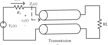
Consider the circuit shown in Fig. 1, wherez1(t) represents the impulse response of the input impedance
of the transmission line (TL) and the variable of interest is the TL’s input current,i1(t).
VS(t) RS i1(t)
RL +
v1(t)
-Z1(t)
Transmission line
Figure 1. Linear circuit used as example.
The circuit is described by (1) in continuous time domain
VS(t) =RSi1(t) +i1(t)∗z1(t) (1)
The process starts by discretizing the continuous time domain equations, under the assumption that the convolved variables are causal, which in this case are z1(t) and i1(t). By doing this, the following
discrete version of Equation (1) is obtained:
VS(ti) =RSi1(ti) + Δt
i
k=0
i1(tk)z1(ti−k) (2)
in whichti represents the discrete time, andi1(ti) denote variablei1evaluated at timeti. Δtrepresents
the sampling time. Afterwards, the discrete equations are solved for the present value of the variables of interest, which in this case is i1(ti). To do so, the discrete convolution on the right-hand side of (2)
is expressed as:
i
k=0
i1(tk)z1(ti−k) =i1(ti)z1(t0) +
i−1
k=0
i1(tk)z1(ti−k) (3)
from which Equation (2) can be rewritten and i1(ti) can be expressed as:
i1(ti) =
VS(ti)−Δt i−1
k=0
i1(tk)z1(ti−k)
z1(t0) Δt+RS
(4)
3. TIME MARCHING INSTABILITY
The stability analysis using the Z-transform is a common technique used in signal processing of discrete signals [13]. In the previous example, if we consider each variable in Equation (2) as a time series, the Z-transform can be applied as follows:
VS(z) =RSI1(z) + Δt·Z1(z)I1(z) (5)
where I1(z) =Z{i1(t)},I2(z) =Z{i2(t)} and Z1(z) =Z{z1(t)}. By solving Equation (5) for I1(z), we
obtain:
I1(z) = VS
(z) Δt·Z1(z) +RS
(6)
which is the Z-domain counterpart of Equation (4).
In Equation (6), it can be seen that the stability ofI1(z) depends on the zeros of its denominator.
If the zeros are outside the unit circle, there are two possible outcomes for i1(ti): either causal and
unstable, or noncausal and stable [13]. Thus, TM yields unstable results if the denominator of any deconvolution equation has at least one zero outside the unit circle since the convolved variables are assumed to be causal. Note, that this assumption enables to limit the summation that replaces the convolution integral, which in turn allows to express the present value of the variable of interest as a function of its past values.
4. RELATION BETWEEN SAMPLING IN THE FREQUENCY DOMAIN AND TIME MARCHING INSTABILITY
It is important to mention that usually in electromagnetic compatibility problems, convolutions are performed between a given variable (voltage, current or wave) and the impulse response of a system. Generally the latter cannot be calculated by analytical means and a numerical approach must be used. For instance, the impulse response of a TL’s input impedance with unmatched load or the admittance parameter of a distributed network.
The process of computing the impulse response of a transfer function with no analytical inverse Fourier transform, usually is composed of: (i) sampling the transfer function, and (ii) applying the IFFT. Note that the sampling in the frequency-domain is related to the Z-domain by:
z=ejωΔt (7)
which means that sampling in the Fourier domain is equivalent to evaluate the Z-domain transfer function on the unit circle. In addition, consider that the process of finding the discrete impulse response by sampling in the frequency domain can only produce zeros in the Z-domain [13]. Thus, the frequency samples determine the zeros position in the Z-domain.
On the other hand, these samples can be affected by phase discontinuity, which refers to the change in phase between the positive and negative spectrum of the frequency samples at the Nyquist frequency. This discontinuity produces oscillations at each discontinuity in time domain, which are less significant if the magnitude near to the discontinuity is close to zero [14]. This means that at−1 in the Z-domain or the Nyquist frequency in the Fourier domain there is an abrupt change in phase, which is seen as a high group delay.
The phase of a given transfer function H(z) composed only by zeros is given by:
θ(z) =
N
k=1
∠z−rkejθk−N∠z (8)
where N is the number of zeros of H(z), and each zero is represented by its polar form rkejθk.
Substituting Equation (7) into Equation (8) in order to express the phase discontinuity in terms of the group delay yields:
−d∠θ(ω)
dω =
N
k=0
Δt−rkΔtcos (θk−ωΔt)
Finally, we evaluate Equation (9) at the Nyquist frequency to obtain:
−d∠θ(ω)
dω
ω=πFS
=
N
k=0
Δt+rkΔtcos (θk)
1 +rk2+ 2rkcos (θk) −NΔt (10)
whereFS is the sampling frequency.
On the other hand, the magnitude due to every zero at the Nyquist frequency is given by:
z−rkejθk
‘ω=πFS
= 2
1 +r2
k+ 2rk+ cos (θk) (11)
It can be seen from Equation (10) that zeros with θk → π and rk → 1 will produce high group delay and hence, high phase discontinuity. However, the same values in Equation (11) will produce low gain. Therefore, if there is phase discontinuity and high gain at the Nyquist frequency, several zeros will appear close to −1 to generate high group delay while some of them will be outside the unit circle to compensate the gain. This behavior was tested by replicating a test depicted in [14], which is described in Appendix A.
In summary, TM will yield unstable responses if the deconvolution equation denominator has frequency samples affected by phase discontinuity with large gain at the Nyquist frequency.
5. PROPOSED SOLUTION TO TM INSTABILITY
In order to prevent the occurrence of zeros outside the unit circle in the denominator of the TM deconvolution equations, we propose to mitigate the phase discontinuity effect in specific parts of the denominator obtained by sampling in the frequency domain. This is done by decreasing their magnitude near the Nyquist frequency.
This was achieved with the following two-step approach. First, each transfer function in the denominator,H(f), obtained by a numerical approach is multiplied by a functionF IX(f) that ensures high attenuation below the Nyquist frequency. Second, the IFFT is applied to this product in order to obtain the stable time series hfix(t):
F−1{
H(f)·F IX(f)}=hfix(t) (12)
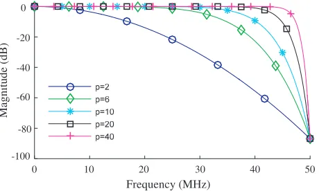
A function of the form e−afp fulfills all the mentioned constraints ifp is even and α is a constant. It is important to mention that the function used in this work is similar to the one used to perform the fast Laplace transform [15], whose form is e−at. Nevertheless, the fast Laplace transform uses its function for casting the frequency samples over a given Laplace contour whereas in our method, the function purpose is being a low pass filter. The following expression forF IX(f) is proposed
F IX(f) =e−k
f
Fs/2
p
(13)
whereFsis the sampling frequency. The parameter kallows selecting the desirable attenuation atFS/2 and phelps to define the frequency above which the attenuation will affect H(f) as depicted in Fig. 2.
6. APPLICATION EXAMPLES 6.1. Linear Circuit
For the circuit shown in Fig. 1, we used the following simulation parameters: the voltage source is represented by a 1-MHz, 5-V peak, sinusoidal signal with an output impedance of 50 Ω. The sampling frequency is 100 MHz and the simulation time 4µs. Two parallel coated wires form the transmission line. The line length is 3 meters, the inner wires radius is 1.075 mm, the thickness of the wires coating is 0.38 mm, and the distance between the two wire centers is 4.35 mm. The relative permittivity of the coating is given by ε = 3 and ε = 0.1886. The TL’s load is 1 kΩ andz1(t) was calculated with 4096
0
-20
-40
-60
-80
-100
Magnitude (dB)
0 10 20 30 40 50
Frequency (MHz)
Figure 2. Magnitude ofF IX(f) as a function ofp withk= 10 andFS = 100 MHz.
1
0.5
0
-0.5
-1
-1.5
Angle (radians)
0 10 20 30 40 50
Frequency (MHz)
Figure 3. Phase of Δt·Z1(z) +RS.
1200
1000
800
600
400
200
Magnitude (
Ω
)
0
10 20 30 40 50
Frequency (MHz)
0
Figure 4. Magnitude of Δt·Z1(z) +RS.
The input voltage of the transmission line was calculated with the following expression:
v1(ti) = Δt
i
k=0
i1(tk)z1(ti−k) (14)
The phase and magnitude obtained the denominator of Equation (6) are shown in Fig. 3 and Fig. 4, respectively. It can be seen that there is a high phase discontinuity and the magnitude at the Nyquist frequency is not low. Hence, unstable zeros are expected in Δt·Z1(z) +RS.
We used the Jury stability criterion for testing if the denominator of Equation (6) has at least one zero outside the unit circle. This criterion was selected because the denominator of Equation (6) has a polynomial degree of 400 for the given simulations parameters,and the algorithms for obtaining the roots of a high degree polynomial (more than 100) are impaired by high inaccuracy [16], whereas the Jury stability criterion is not affected by this [17]. In this case the Jury criterion predicted unstable results.
We compared the TM results against numerical results obtained using CST Cable Studio, which are shown in Fig. 5 and Fig. 6. It can be seen that the unstable behavior is present in both variables at late time.
We only applied our solution over Z1(f) because it is the part of the denominator of Equation (6)
10
5
0
-5
-10
Amplitude (mA)
0 0.5 1 1.5 2 2.5
Time (μs)
3 3.5 4
Figure 5. Currenti1(t) calculated using TM and
CST Cable Studio.
5
0
-5
Voltage (V)
0 0.5 1 1.5 2 2.5
Time (μs)
3 3.5 4
Figure 6. Voltage v1(t) calculated using TM and
CST Cable Studio.
1
0.5
0
-0.5
-1
-1.5
Angle (radians)
0 10 20 30 40 50
Frequency (MHz)
Figure 7. Phase of fixed Δt·Z1(z) +RS.
1200
1000
800
600
400
200
Magnitude (
Ω
)
0
10 20 30 40 50
Frequency (MHz)
0
Figure 8. Magnitude of fixed Δt·Z1(z) +RS.
10
5
0
-5
-10
Amplitude (mA)
0 0.5 1 1.5 2 2.5
Time (μs)
3 3.5 4
Figure 9. Current i1(t) calculated using stable
TM and CST Cable Studio.
6
0
-2
Voltage (V)
0 0.5 1 1.5 2 2.5
Time (μs)
3 3.5 4
-6 2
-4 4
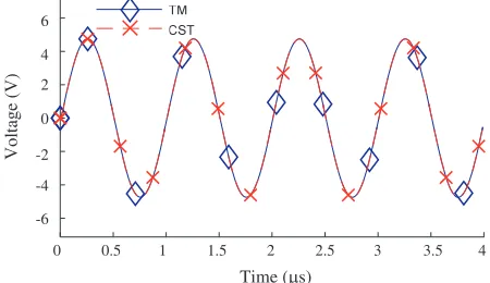
Figure 10. Voltage v1(t) calculated using stable
TM and CST Cable Studio.
6.2. Nonlinear Example
For this example, we used the circuit shown in Fig. 11. The output impedance of the voltage source was set to 10 Ω, the line load and length are 2 kΩ and three meters, respectively. The diode was represented by its voltage-current relationship given by:
iD(t) =IS
e
vD
ηvt
VS(t)
RS
i1(t)
RL
+ v1(t)
-Z1(t)
i2(t)
Transmission line
Figure 11. Circuit with a nonlinear device.
10 5 0 -5 -10 Amplitude (mA)
0 0.5 1 1.5 2 2.5
Time (μs)
Figure 12. Current i1(t) calculated using TM
and CST Cable Studio.
600 500 400 300 200 100 0 -100 Amplitude (mA)
0 0.5 1 1.5 2 2.5
Time (μs)
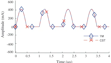
Figure 13. Current iD(t) calculated using TM and CST Cable Studio.
whereIs= 5.31656A, η = 2 andvt = 25 mV. The rest of the simulation parameters are equal to those used in the previous example.
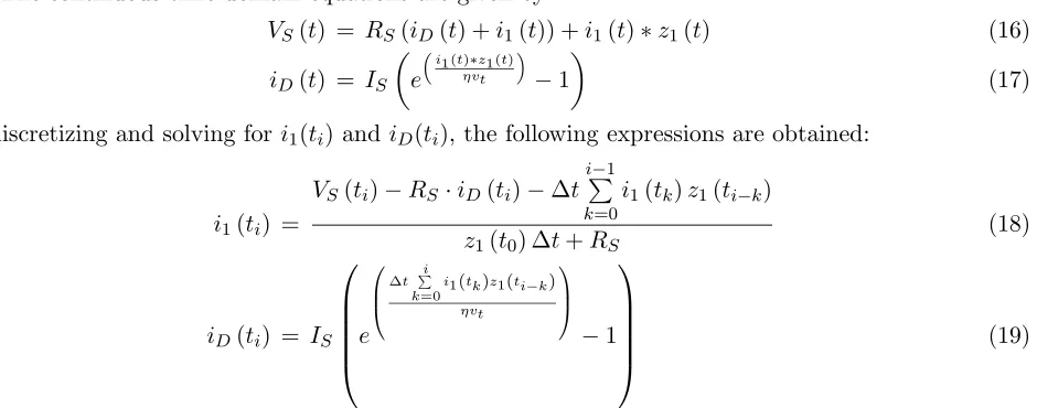
The continuous time domain equations are given by:
VS(t) = RS(iD(t) +i1(t)) +i1(t)∗z1(t) (16)
iD(t) = IS
e
i
1(t)∗z1(t)
ηvt
−1 (17)
By discretizing and solving fori1(ti) and iD(ti), the following expressions are obtained:
i1(ti) =
VS(ti)−RS·iD(ti)−Δti− 1
k=0
i1(tk)z1(ti−k)
z1(t0) Δt+RS
(18)
iD(ti) = IS
⎛ ⎜ ⎜ ⎜ ⎜ ⎝e ⎛ ⎜ ⎝
Δt i
k=0i1(tk)z1(ti−k)
ηvt ⎞ ⎟ ⎠ −1 ⎞ ⎟ ⎟ ⎟ ⎟ ⎠ (19)
It is important to notice that in this example, it is not possible to solve analytically Equations (4) and (19) for both unknowns. Hence, we solved them by using the Newton-Raphson method at each iteration.
Then, Equation (18) performs the deconvolution operation and its Z-transform is
I1(z) = VS
(z)−ID(z)RS
Δt·Z1(z) +RS
(20)
Note that Equation (20) is expressed in terms of ID(z) because nonlinear operator such as the one
10
5
0
-5
-10
Amplitude (mA)
0 0.5 1 1.5 2 2.5
Time (μs)
3 3.5 4
Figure 14. Currenti1(t) calculated using stable
TM and CST cable studio.
0 0.5 1 1.5 2 2.5
Time (μs)
3 3.5 4
600
400
200
0
-600
Amplitude (mA) -200
-400
Figure 15. CurrentiD(t) calculated using stable TM and CST cable studio.
We applied the proposed method withk= 10 and p= 20 in order to increase the cutoff frequency and include more harmonics. The results of TM and CST Cable Studio are shown in Fig. 14 and Fig. 15. It can be seen that there is excellent agreement between TM and CST results. The differences may be partially explained by the fact that in CST Cable Studio, transmission lines are modeled as an equivalent circuit composed of a finite number of elementary cells.
Finally, it should be noted that the effectiveness of the proposed solution could be compromised if time aliasing is not properly considered.
7. CONCLUSIONS
We identified in this work one cause of instability in the TM method, which is related to the calculation of variables involved in a convolution. We showed that this instability is related to the phase discontinuity. We also provided a solution to this problem, which prevents the appearance of Z-domain unstable poles. This solution is fundamentally different from other previously presented approaches in the sense that it is not a filtering or predicting technique applied during the TM run. Instead, it consists of a preprocessing procedure on the denominators of the deconvolution equations. The proposed solution consists of imposing high attenuation on the transfer function prior the half of the sampling frequency in order to decrease the effect of the phase discontinuity.
The efficiency of the proposed method was illustrated using two examples involving a transmission line with linear or non-linear elements. The method can find useful applications in various fields such as electromagnetic compatibility, signal integrity, and transmission line analysis.
We recommend using the Jury test for predicting the stability of TM, without running TM simulations, which is especially useful for cases with nonlinear devices. Furthermore, the test does not require finding the roots of a high degree-polynomial or the exact position of the zeros.
APPENDIX A.
In [14], the effect of phase discontinuity was explained in time and frequency domains by comparing the impulse response of a low-pass RC filter. Two methods were used to obtain the impulse response:
• Method 1: the impulse response of the continuous time domain was discretized.
• Method 2: the transfer function was discretized and then transformed in time domain by using the IFFT.
Hence, the phase discontinuity only occurs in Method 2 [14].
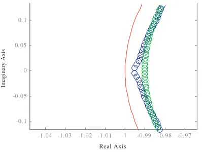
In our case, we were interested in the effects of phase discontinuity in the Z-domain. Thus, we compared the Z-transform of both time series.
Real Axis
Imaginary Axis
-1.04 -1. 03 -1.02 -1.01 -1 -0.99 -0. 98 -0.97 -0.1
-0.05 0 0. 05 0. 1
Figure A1. Zeros of the impulse response of a low-pass RC filter with τ = 10µs, sampling frequency of 10 MHz and 200 frequency points. The unit circle is shown in red. The green and blue circles depict zeros of the impulse response without and with phase discontinuity, respectively.
shown in Fig. A1. It can be seen that the zeros of an impulse response with phase discontinuity have the behavior described in Section 4.
REFERENCES
1. Tesche, F. M., “On the analysis of a transmission line with nonlinear terminations using the time-dependent BLT equation,” IEEE Transactions on Electromagnetic Compatibility, Vol. 49, No. 2, 427–433, May 2007.
2. Rao, S. M., Time Domain Electromagnetics, Academic Press, 1999.
3. Taflove, A., Computational Electrodynamics: The Finite-difference Time-domain Method, 1st edition, Artech House, 1995.
4. Tijhuis, A. G., “Toward a stable marching-on-in-time method for two-dimensional transient electromagnetic scattering problems,” Radio Science, Vol. 19, No. 5, 1311–1317, Sep. 1984.
5. Shi, Y., M.-Y. Xia, R. Chen, E. Michielssen, and M. Lu, “A stable marching-on-in-time solver for time domain surface electric field integral equations based on exact integration technique,” 2010
IEEE Antennas and Propagation Society International Symposium (APSURSI), 1–4, 2010.
6. Bin Sayed, S., H. A. Ulku, and H. Bagci, “A stable marching on-in-time scheme for solving the time-domain electric field volume integral equation on high-contrast scatterers,”IEEE Transactions on Antennas and Propagation, Vol. 63, No. 7, 3098–3110, Jul. 2015.
7. Smith, P. D., “Instabilities in time marching methods for scattering: Cause and rectification,”
Electromagnetics, Vol. 10, No. 4, 439–451, Oct. 1990.
8. Rynne, B. P. and P. D. Smith, “Stability of time marching algorithms for the electric field integral equation,” Journal of Electromagnetic Waves and Applications, Vol. 4, No. 12, 1181–1205, Jan. 1990.
9. Sadigh, A. and E. Arvas, “Treating the instabilities in marching-on-in-time method from a different perspective [electromagnetic scattering],” IEEE Transactions on Antennas and Propagation, Vol. 41, No. 12, 1695–1702, Dec. 1993.
10. Lacik, J., Z. Lukes, and Z. Raida, “Signal processing techniques for stabilization of marching-on-in-time method,” International Conference on Electromagnetics in Advanced Applications, 2009, ICEAA’09, 670–673, 2009.
12. Ulku, H. A., H. Bagci, and E. Michielssen, “Marching on-in-time solution of the time domain magnetic field integral equation using a predictor-corrector scheme,” IEEE Transactions on Antennas and Propagation, Vol. 61, No. 8, 4120–4131, Aug. 2013.
13. Proakis, J. G. and D. G. Manolakis, Digital Signal Processing: Principles, Algorithms, and Applications, Prentice Hall, 1996.
14. Pupalaikis, P. J., “The relationship between discrete-frequency s-parameters and continuous-frequency responses,”Design Con., 1–28, Santa Clara, CA, 2012.
15. Bertholet, P. F. and F. M. Tesche, “The fast laplace transform,” Sep. 6, 2009.
16. Priyanka, B., S. Panwar, and S. D. Joshi, “Finding zeros for linear phase FIR filters,”2013 IEEE 3rd International Advance Computing Conference (IACC), 1103–1107, 2013.