Measurement Methodologies for Reducing Errors in the Assessment
of EMF by Exposimeter
Rodrigues Kwate Kwate1, *, Bachir Elmagroud1, Chakib Taybi1, Veronique Beauvois2, Christophe Geuzaine2, Dominique Picard3, and Abdelhak Ziyyat1
Abstract—Objective: As well known, using a single body worn sensor exposimeter introduces systematic errors on the measurement of the incident free space electric field strength. This is because the body creates around it high, intermediate and low level field zones, which depend on the direction of arrival of the incident field. The goal of this work is to propose an efficient method for the reduction of these errors. Methods: After classifying the perturbations induced by the body on the measured electric and magnetic fields thanks to realistic numerical simulations, we then propose a two-sensor setup in conjunction with simple semi-empirical correction formulas, in order to compensate these perturbations. Results: At 942 MHz, when the two sensors are placed in any opposite sides of the body at chest height, the worst case, maximum and average errors respectively decrease to 12% and 3% compared to 83% and 22% for measurement techniques using a single sensor, or 32% and 11% when using the average value of the measurements. Conclusion: The error related to the measurement in the presence of the body was significantly reduced by the proposed method making use of two opposite sensors, E-field and H-field at the chest. Significance: The conformity of exposure to EMF in terms of reference values according to the ICNIRP is given in the abscence of the human body. The interest of this work lies in the reduction of the errors made when measuring the field in the presence of the body.
1. INTRODUCTION
The International Commission on Non-Ionizing Radiation Protection (ICNIRP) [1] provides scientific advice and guidance on the health and environmental effects of non-ionizing radiation (NIR) to protect people and environment from detrimental NIR exposure. Two classes of guidance are provided, basic restrictions and reference levels. The basics restrictions use specified physical quantities (Current density and specific energy absorption rate) for directly established health effects. The references levels are provided for practical exposure assessment purposes to determine whether the basic restrictions are likely to be exceeded. All reference levels are derived from relevant basic restrictions using measurement and/or computational techniques, and some address perception and adverse indirect effects of exposure to EMF. The derived quantities are electric field strength (E), magnetic field strength (H), magnetic flux density (B) and power density (P). In any particular exposure situation, measured or calculated values of any of these quantities without body presence can be compared with the appropriate reference level. Compliance with the reference level will ensure compliance with the relevant basic restriction. In this paper, we will focus on the techniques for measuring E by radiofrequency exposimeter. Many studies also measure E or H in order to verify that the reference levels provided are not exceeded [2–9]. The ICNIRP guidelines [1] also specify that if the measured value exceeds the reference level, it does
Received 26 June 2017, Accepted 4 August 2017, Scheduled 12 August 2017
* Corresponding author: Rodrigues Kwate Kwate ([email protected]).
1 Electronic and Systems Laboratory, Faculty of Sciences, Mohammed Premier University, Oujda, Morocco. 2 Applied and
not necessarily follow that the basic restriction will be exceeded. However, whenever a reference level is exceeded it is necessary to test compliance with the relevant basic restriction and to determine whether additional protective measures are necessary. Furthermore, the measurement of E is an important step which can condition the measurement of the Specific Absorption Rate (SAR) or not. Indeed, generally, it is more advisable to measure E and compare it to the reference levels in order to assess the EMF exposure. The problem about which this work is concerned comes from the fact that the measurement of E is carried out by the worn body exposimeter, whereas the reference values are given in the absence of any body. The objective of this work is to go back to the reference value of the ICNIRP from the measurement of the field in the presence of the human body.
Several studies aiming to quantify the influence of the human body on the exposimeter measurements have been published over the last decade. It is shown in [10] and [11] that the body can produce attenuations up to 30 dB at 900 MHz. The errors due to the position of the exposimeter on the body were shown to be significant in [8], with ten exposimeter positions considered (six around the waist, two on arms and two on the upper back). The study also showed the effect of frequency on the measurement error. Finally, a thorough investigation of the influence of the body for several frequency bands is presented in [9]. A number of techniques have been proposed to attenuate the EMF assessment error linked with the presence of the human body. The method proposed in [12] uses numerical simulations to estimate an average electric field and Specific Absorption Rate (SAR). The number of measurement points used in this technique is not fixed, and the method requires the knowledge of the frequency to determine the dielectric constant of each internal organ of the body before calculating the SAR. The technique cannot readily be used in practice because of the large number of sensors necessary for reliable EMF assessment. A Personal and Distributed Exposimeter (PDE) with measurements at different locations on the human body is presented in [13]. The predicted average error is 7% for 10 sensors, 13% for 3 sensors and 16% for 2 sensors. This distributed measurement approach is interesting but relies on the a priori knowledge of the ambient electromagnetic fields. Moreover, the maximum errors obtained for each combination are not reported.
Throughout this analysis, an exposimeter is materialized by a single or several sensors distributed around the human body and all connected to one processing system. Discussions will only focus on the number of sensors connected to the same processing system. The main objective of this work is to propose an efficient methods for error reducing when EMF level is to be assessed in the vicinity of human body. The following three questions are examined:
(1) What are the errors related to this assessment in the vicinity of the human body when using a single sensor exposimeter? How to qualify and quantify these errors?
(2) When several measurements sensors are used, how should they be chosen and combined? What is the impact of the number of sensors on the measurement performance? Is there an optimum number of sensors? The optimal number is the number from which the error can no longer be significantly reduced.
(3) Is it interesting to measureH in addition toE in order to evaluate EMF exposure?
This paper is organized as follows. In Section 2, we identify and classify errors due to the presence of the body. Section 3 presents error mitigation techniques. Several approaches are studied, based on distributed sensors for a single exposimeter and/or a combination of electric field and magnetic field (E, H) measurements. Two performance indicators are considered: the maximum and the average errors due to human body. A method based on a two-sensor setup in conjunction with simple semi-empirical correction formulas is recommended, as it provides a good compromise between accuracy and ease of implementation. Section 4 presents numerical and experimental results, validating the proposed methodology.
2. EXPOSURE ASSESSMENT ERRORS DUE TO BODY PROXIMITY
2.1. Electromagnetic Field around the Body
(a) (b)
Figure 1. GUSTAV human body model (from CST Studio). (a) Heterogenous whole body model. (b) Homogeneous torso model without arms.
Figure 2. Locations of field evaluation points. Chest (hC = 143 cm, R1 = 28 cm, R2 = 17 cm),
abdomen (hA = 125 cm, R1 = 28 cm, R2 = 20 cm) and waist (hW = 110 cm, R1 = 19 cm, R2 = 18 cm);
Li,kLi,k+1 =Li,kLi,1 =ϕ (Angle between two consecutive points used for field measurement) ; R1 and R2 are respectively the major and minor radii of ellipses defined for each measurement height.
use the heterogeneous human body model [16] (GUSTAV, man, 176 cm, 69 kg, 38 years): see Figure 1 (Page 3). The exposure consists in a plane wave with 1 Vm−1 electric field. The magnitudes of the electromagnetic fields (EPi and HPi) are evaluated on N points Pi (i = 1, . . . , N) located on ellipses
around the body, at three different heights — around the chest, abdomen and waist (see Figure 2). These fields are provided by CST studio.
2.2. Error Definitions
Let EPbody
i denote the strength of the electric field at pointPi with the presence of body andE
free
Pi the
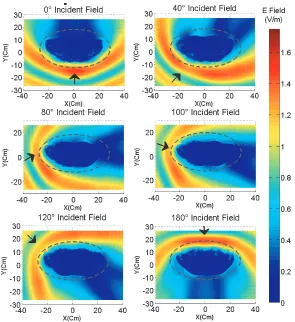
undisturbed electric field strength at the same point in the absence of human body as recommended by the ICNIRP [1]. Indeed, the strength of the electric field is measured in free space at a given location which will then be compared to the reference levels in order to check compliance with standards. Figure 3 shows three major zones in each incident field scenario:
• The zone where theE-field is greater than the incident one for vertical and horizontal polarizations. This is the reflection zone SR ={Pi :EPbody
i > E
free
Pi }. We donote by NR the number of points in this zone, in which we will define aBody Reflection Error (BRE).
Figure 3. Electric field strength at chest height. The arrow represents the incident field direction (with vertical polarization).
values represent the measurement points in the shadowing zoneSS ={Pi :EPbody
i <0.3E
free
Pi }. We
denote byNS the number of points in this zone, in which we define aBody Shadowing Error (BSE).
This error is the most important one when using an exposimeter to evaluate the EMF. Some work has already tried to quantify this error [2, 3].
• Between the two previous zones, the diffraction zone SD ={Pi : 0.3.Efree
Pi ≤ E
body
Pi ≤ E
free
Pi }. We
denote byND the number of points in this zone, in which we defineBody Diffraction Error (BDE). The errors in the different zones are defined as follows:
BRE = 100
NR
Pi∈SR
Efree
Pi −E
body
Pi
Efree
Pi
(1)
BSE = 100
NS
Pi∈SS
Efree
Pi −E
body
Pi
Efree
Pi
(2)
BDE = 100
ND
Pi∈SD
Efree
Pi −E
body
Pi
Efree
Pi
(3)
In addition to these zone errors, we define a Body Depolarization average Error (BPE), which quantifies the depolarization due to the body. If the incident field is polarized vertically, we define
BPEH =
100
N
N
i=1 Ebody
H,Pi
Efree
Pi
whereEH,Pbodyi =
Ebody
x,Pi
2
+Ey,Pbodyi 2, andN, used in Equations (4), (5) and (6), is the variable of number of points in which strength of field is evaluated, as mentioned on this page, at the beginning of first column. If the incident field is polarized horizontally, we define
BPEV = 100
N
N
i=1 Ebody
⊥,Pi
Efree
Pi
, (5)
whereEbody⊥,P
i is the field in the plane orthogonal to the incident polarization. Finally, we define theBody average Error (BE) as follows:
BE = 100
N
N
i=1 Efree
Pi −E
body
Pi
Efree
Pi
(6)
In addition to these average errors, we will also report the maximum, pointwise errors that are obtained with each of the proposed methods. Indeed, the determination of the electric field strength with precision will make it possible in practice to compare it with the reference values, in order to verify compliance with standards that regulate people’s exposure to electromagnetics fields.
3. ERROR MITIGATION TECHNIQUES
We propose two families of error mitigation techniques:
3.1. Multi-Coefficient Method
The multi-coefficient method is based on multiple linear regression analysis, which attempts to model the relationship between two or more explanatory variables and a response variable by fitting a linear equation to observed data. Here, we look for a relation between the values measured in the presence of human body and the values measured in free space. To obtain this relation, it is necessary to determine the regression coefficients (vector A) that minimize the residual (vector Ra). For each situation, the vector Ais obtained based on the numerical calculations carried out by the codes that we have written with Matlab:
Efree =XbodyA+Ra, (7)
with
Efree =
⎛ ⎜ ⎜ ⎜ ⎜ ⎜ ⎜ ⎝ 1 EPfree1 ..
. ...
i Efree
Pi ..
. ...
N Efree
PN ⎞ ⎟ ⎟ ⎟ ⎟ ⎟ ⎟ ⎠
; A=
⎛ ⎜ ⎜ ⎜ ⎜ ⎜ ⎝ 1 a1 .. . ...
k ak
.. . ...
K aK
⎞ ⎟ ⎟ ⎟ ⎟ ⎟ ⎠ . (8)
The Xbody matrix is composed by N rows and K columns. The different methods are based
on the possibility of measuring four different quantities, all in V/m. For any (i, k) position on the measuring ellipse (Figure 2), we can measure, V1bodyL
i,k = E
body
Li,k , V2
body
Li,k = Z0 ×H
body
Li,k , V3
body
Li,k =
max(ELbody
i,k , Z0×H
body
Li,k ) andV4
body
Li,k = (E
body
Li,k +Z0×H
body
Li,k )/2. So, the (i, k) entryx
body
Li,k in this matrix is defined as:
xbody
Li,k =
⎧ ⎪ ⎪ ⎪ ⎪ ⎪ ⎨ ⎪ ⎪ ⎪ ⎪ ⎪ ⎩
V1bodyL
i,k [M11]
V2bodyL
i,k [M12]
V3bodyL
i,k [M13]
V4bodyL
i,k [M14]
where Z0 ≈ 120×π ≈ 376.99 Ω is the wave-impedance of a plane wave in free space, and ELbody i,k and
Hbody
Li,k are respectively the electric field strength and the magnetic field strength measured at the Li,k position on the body. M11, M12, M13 and M14 denote the different ways to consider xbodyL
i,k in the multi-coefficient method.
The residual vector Ra contains the N errors terms: the maximum error is Ramax= max(Rai), and the average error isRamean= mean(Rai),i= 1, . . . , N.
3.2. Single-Coefficient Method with Maximum Value
The single-coefficient method is based on a simple linear regression:
Efree =b Ybody+Rb (10)
whereb is the single correction factor and where the i-th entryybodyP
i in the vector Y
body is defined as:
ybody
Pi =
⎧ ⎪ ⎪ ⎪ ⎪ ⎪ ⎨ ⎪ ⎪ ⎪ ⎪ ⎪ ⎩
max(V1bodyL i,1 , ..., V1
body
Li,K) [M21]
max(V2bodyLi,1 , ..., V2bodyLi,K) [M22] max(V3bodyL
i,1 , ..., V3
body
Li,K) [M23]
max(V4bodyL i,1 , ..., V4
body
Li,K) [M24]
(11)
In this method, we take maximum quantity for all the K points used in measuring ellipse. The residual vectorRb contains theN error terms. As for the multi-coefficient method, the maximum error
is Rb
max = max(Rb), and average error is Rbmean = mean(Rb). M21, M22, M23 and M24 denote the
different ways to consider ybody in the single-coefficient method.
In addition to the eight methods described above, we also consider method M00, which represents a conventional measurement technique using a single sensor, as well as methods M10 and M20, which represent the simple cases when we just measure the electric field in a two-sensor setup, either by averaging the values (M10) or taking the maximum value (M20). M10 is also used in [13].
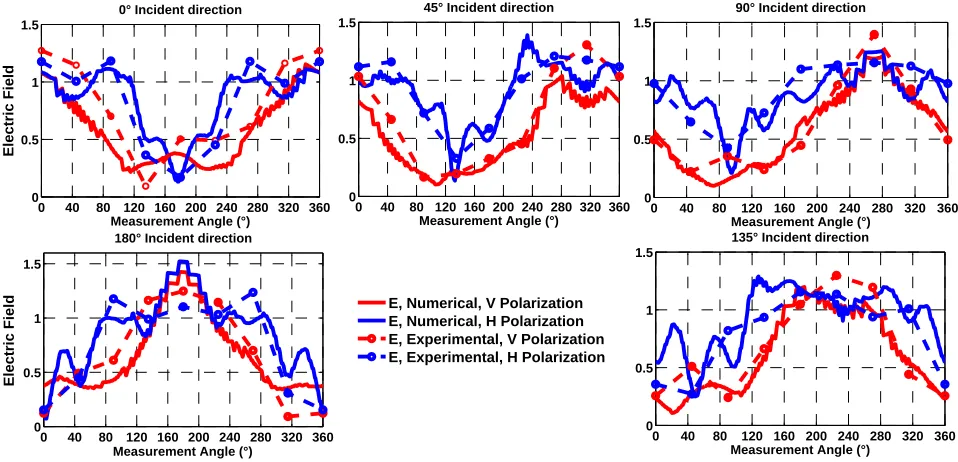
4. RESULTS AND DISCUSSION
4.1. Comparison between Simulations and Measurements
Figure 4. Measurement validation tools: antenna, probe and human body model.
0 40 80 120 160 200 240 280 320 360 0
0.5 1 1.5
0° Incident direction
Electric Field
Measurement Angle (°)
0 40 80 120 160 200 240 280 320 360 0
0.5 1 1.5
45° Incident direction
Measurement Angle (°) 0 40 80 120 160 200 240 280 320 360 0
0.5 1 1.5
90° Incident direction
Measurement Angle (°)
0 40 80 120 160 200 240 280 320 360 0
0.5 1 1.5
135° Incident direction
Measurement Angle (°) 0 40 80 120 160 200 240 280 320 360
0 0.5 1 1.5
180° Incident direction
Measurement Angle (°)
Electric Field
E, Numerical, V Polarization E, Numerical, H Polarization E, Experimental, V Polarization E, Experimental, H Polarization
Figure 5. Comparison between measurements and simulations at 942 MHz.
4.2. Body Errors Classification for a Single Point
The variation of the intensity of the electric (E) and magnetic (H) fields along the axis OY at height
z = hc is shown in Figure 6. The intensity of the electric field varies from 0.51 V/m on the surface of the human body, to 1.47 V/m at 17.4 cm distance from the surface of the body. The intensity of the magnetic field changes from 3.93 10−3A/m at the surface of the human body to 1.26 10−3A/m
-200 -15 -10 -5 0 5 10 15 20 0.125 0.25 0.375 0.5 0.625 0.75 0.875 1 1.125 1.25 1.375 1.5 y (cm)
E ( V/m)
0° incident field direction , V Polarization
-200 -15 -10 -5 0 5 10 15 20
0.125 0.25 0.375 0.5 0.625 0.75 0.875 1 1.125 1.25 1.375 1.5 1.6251.7 y (cm)
E ( V/m)
0° incident field direction , H Polarization
-200 -15 -10 -5 0 5 10 15 20
0.5 1 1.5 2 2.5 3 3.5 4 4.5
5x 10
3
y (cm)
H ( A/m)
0° incident field direction , V Polarization
-200 -15 -10 -5 0 5 10 15 20
0.5 1 1.5 2 2.5 3 3.5 4 4.5
5x 10
3
y (cm)
H ( A/m)
0° incident field direction , H Polarization
400 MHz, 942 MHz, 1842 MHz
Incident field direction Human Body Human Body Human Body Human Body
Figure 6. Variation ofE andH fields along the OY axis at heightz=hc= 143 cm with the presence
of human body. For 400 MHz, 942 MHz and 1842 MHz.
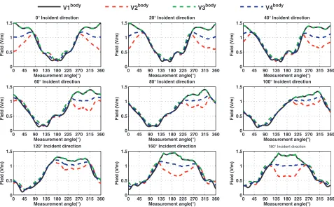
This observation can also be made with the measuring ellipse in the direction of arrival of the field or reflection zone (Figure 7). These remarks allow us to imagine that an exposimeter worn on the front and capable of simultaneously measuring both electric and magnetic components will be less susceptible to under-estimating the incident field strength (when arriving from the front) due to a null in one of the components caused by destructive interference. However, an under-estimation in both components of the field cannot be avoided when an exposimeter is located at the rear where the body shields the exposimeter from the front incident plan wave. Overall, similar variability in the electric and magnetic field strengths close to the body is observe.
We classify assessment errors due to the presence of the body and present an assessment based on the combination approach (distributed measurements, electric and magnetic fields). As shown in [10, 11] and [17–19], using a single sensor is largely ineffective in an overall estimation exposure. Indeed, Figures 3 and 7 show the field level around the chest for different incident fields direction. Particularly in Figure 7, we compare four fields quantities with the incident field in free space such as:
E-field with body presence V1body, V2body, V3body and V4body. This shows how V1body and V3body curves match for on all diagrams, and there is noticeable difference betweenV2body,V4bodyandV1body curves, in central parts of diagrams regarding direction of arrival of incident field. This can be explained by the result obtained in Figure 6. Indeed, at a distance from the human body less than a quarter of the wavelength of the incident field (7.75 cm for 942 MHz), opposite to the direction of arrival of the incident field, V1body ≈ V3body ≈ max(Ebody, Z0Hbody) because Ebody > Z0Hbody, and at the rear side (back) of the human body relative to direction of arrival, Ebody and Z0Hbody are both very low.
On the other hand, it can be seen that the two fields E and Z0×H act in a complementary manner around the reference value, hence the interest to study the measured values as the average defined by (E +Z0 ×H)/2. Relative to this observations, a measurement method based on multiple points distributed in the reflection, diffraction and shading zones is required.
0 45 90 135 180 225 270 315 360 0
0.5 1 1.5
Measurement angle(°)
Field (V/m)
0° Incident direction
0 45 90 135 180 225 270 315 360 0
0.5 1 1.5
Measurement angle(°)
Field (V/m)
20° Incident direction
0 45 90 135 180 225 270 315 360 0
0.5 1 1.5
Measurement angle(°)
Field (V/m)
40° Incident direction
0 45 90 135 180 225 270 315 360 0
0.5 1 1.5
Measurement angle(°)
Field (V/m)
60° Incident direction
0 45 90 135 180 225 270 315 360 0
0.5 1 1.5
Measurement angle(°)
Field (V/m)
80° Incident direction
0 45 90 135 180 225 270 315 360 0
0.5 1 1.5
Measurement angle(°)
Field (V/m)
100° Incident direction
0 45 90 135 180 225 270 315 360 0
0.5 1 1.5
Measurement angle(°)
Field (V/m)
120° Incident direction
0 45 90 135 180 225 270 315 360 0
0.5 1 1.5
Measurement angle(°)
Field (V/m)
160° Incident direction
0 45 90 135 180 225 270 315 360 0
0.5 1 1.5
Measurement angle(°)
Field (V/m)
180° Incident direction
V1body V2body V3body V4body
Figure 7. Elliptical scanning at chest height of the human body (Vertical polarization, 942 MHz).
Figure 8. BoxPlot explanation.
-70 -60 -50 -40 -30 -20 -10 0 10 20 30 40 50 60 70 80 90 100
BRE_C BDE_C BSE_C BPE_H_CBE_C BRE_A BDE_A BSE_A BPE_H_ABE_A
BRE_W BDE_W BSE_WBPE_H_WBE_W
Errors due to human body vicinity (%)
Chest Abdomen Waist
Figure 9. Assessment Errors due to proximity of the Body (Vertical polarization).
-100 -90 -80 -70 -60 -50 -40 -30 -20 -10 0 10 20 30 40 50 60 70 80 90 100
BRE_C BDE_C BSE_C BPE_V_C BE_C BRE_A BDE_A BSE_A BPE_V_A BE_A BRE_W BDE_W BSE_WBPE_V_W BE_W
Errors due to human body vicinity (%)
Waist Abdomen
Chest
Figure 10. Assessment Errors due to proximity of Body (Horizontal polarization).
gives the behavior of all the situations, hence the values of interest such as IQRand Δ.
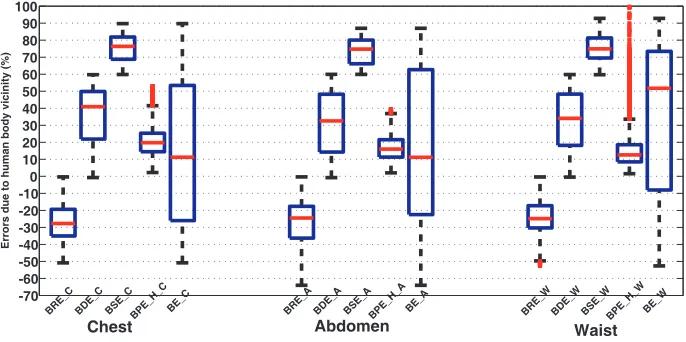
We also notice that errors due to reflection of the incident field by the body are mostly over-estimated. Indeed, the boxplots representing all theBRE are mostly in the negative part of the graph. Moreover, theirIQR between 13% and 24% means that nearly 50% of the measured samples are quite close within 25% of their median value, the median value that varies between 15% and 27% (i.e., between 1.15 V/m and 1.27 V/m). In other words, in vertical polarization, half of the measurements made in the reflection zone is between 1 V/m and 1.15 V/m, and the other half is more than 1.15 V/m. In horizontal polarization, half of the measurements made in the reflection zone is between 1 V/m and 1.27 V/m, and the other half is more than 1.27 V/m. The maximum difference between the errors due to the reflection of the incident field by the human body (Δ) is between 0% and 63% (between 1 V/m and 1.63 V/m) and particularly between 0% and 85% (between 1 V/m and 1.85 V/m) for horizontal polarization and for measurements made at the waist level. In terms of outliers, we notice that they are usually present when it comes to make measurements in the waist zone. This is due to the presence of the arms in this region. Indeed, when we approach the zone of the chest, this is reduced considerably; it can also be noticed that, as we presented in [19], the chest zone is the most stable zone and most recommended for assessment of personal body exposure. On the other hand, while making these remarks, the outliers do not represent more than 6% (BP E V W horizontal polarization) of all the measurements carried out. This reflects the fact that the data are quite clustered in the boxplot.
4.3. Error Mitigation Results
ForK measurement points (φ= 360◦/K), we show in Figure 11 how the average error (BE) decreases with the increase of the number of points (K). This extends the results that we presented in [19] and [20] for two measurement points. When the number of measuring points increases, it is possible to get at least one point in the reflection or diffraction zones, and the average of measurements will be closer to the free space value of the field: for chest height and vertical polarization, we have IQR= 30% and Δ = 89% for a single point, IQR= 12% and Δ = 36% for 2 points, IQR= 11% and Δ = 28% for 3 points and
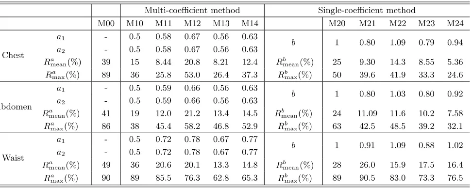
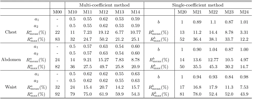
IQR = 8% and Δ = 28% for 4 points. In other words, after three points or sensors, it is no longer necessary to increase the sensors because the impact on the performance of the measurement is no longer very significant. These observations are also clearly shown in Tables 1 and 2 and Figure 12. Indeed, with the method that we propose (M24), we obtain the best error reduction for only two measurement
-15 0 15 30 45 60 75 90 100
BE_C_1BE_C_2BE_C_3BE_C_4 BE_A_1BE_A_2BE_A_3BE_A_4 BE_W_1BE_W_2BE_W_3BE_W_4
Error due to Human Body Vicinity (%)
Vertical polarization
-15 0 15 30 45 60 75 90 100
BE_C_1BE_C_2BE_C_3BE_C_4 BE_A_1BE_A_2BE_A_3BE_A_4 BE_W_1BE_W_2BE_W_3BE_W_4
Error due to Human Body Vicinity(%)
Horizontal polarization Chest
Chest
Abdomen
Abdomen Waist
Waist
Figure 11. Assessment errors based on simultaneouslyK measurements points, average combination.
-25 0 25 50 75 100
BE_C_M00BE_C_M10BE_C_M20BE_C_M11BE_C_M21BE_C_M13BE_C_M24 BE_A_M00BE_A_M10BE_A_M20BE_A_M11BE_A_M21BE_A_M13BE_A_M24 BE_W_M00BE_W_M10BE_W_M20BE_W_M11BE_W_M21BE_W_M13BE_W_M24
Error due to Human Body Vicinity (%)
Vertical polarization
-25 0 25 50 75 100
BE_C_M00BE_C_M10BE_C_M20BE_C_M11BE_C_M21BE_C_M13BE_C_M24 BE_A_M00BE_A_M10BE_A_M20BE_A_M11BE_A_M21BE_A_M13BE_A_M24 BE_W_M00BE_W_M10BE_W_M20BE_W_M11BE_W_M21BE_W_M13BE_W_M24
Error due to Human Body Vicinitys
(%-)
Horizontal polarization
Figure 12. Comparison between the assessment errors obtained for the different techniques M00 (BE M00), M10 (BE M10), M20 (BE M20), M11 (BE M11), M21 (BE M21), M13 (BE M13) and M24 (BE M24).
points (Reduction of 8 times in terms of average error and 3 to 7 times in terms of maximum error). We also note that, for a singleE-field sensor, regardless of the measurement level (chest, abdomen and waist), the behaviors of average and maximum errors are the same. For conventional measurement methods with two E-field sensors, M10 (average method) and M20 (maximum method) are described in the last paragraph of Section 3.2 (Single-coefficient Method with Maximum Value).
It is necessary to avoid making measurements at the waist level, because it presents twice as many errors as the other positions (Chest and abdomen) with a slight preference for chest level. The robustness of M24 method compared to others is due to the combination of E-field and H-field with two points diametrically opposed to the measuring ellipse. This result considerably reduces the complexity of the exposimeter presented in [13]. Several exposimeters as ESM-30 RADMAN XT already measure the electric and magnetic fields. By combining two sensors of this exposimeter with the M24 method, we will get 3% average error and 12% maximum error in free space electric field strength assessment.
Table 1. Correction parameters for vertical polarization and two measurement points.
Multi-coefficient method Single-coefficient method
M00 M10 M11 M12 M13 M14 M20 M21 M22 M23 M24
Chest
a1 - 0.5 0.58 0.67 0.56 0.63 b
1 0.80 1.09 0.79 0.94
a2 - 0.5 0.58 0.67 0.56 0.63
Ra
mean(%) 39 15 8.44 20.8 8.21 12.4 Rmeanb (%) 25 9.30 14.3 8.55 5.36
Ra
max(%) 89 36 25.8 53.0 26.4 37.3 Rbmax(%) 50 39.6 41.9 33.3 24.6
Abdomen
a1 - 0.5 0.59 0.66 0.56 0.63
b 1 0.80 1.03 0.80 0.92
a2 - 0.5 0.59 0.66 0.56 0.63
Ra
mean(%) 41 19 12.0 21.2 13.4 14.5 Rbmean(%) 24 11.09 11.6 10.2 7.58
Ra
max(%) 86 38 45.4 58.2 46.8 52.9 Rbmax(%) 63 42.5 48.5 39.2 32.1
Waist
a1 - 0.5 0.72 0.78 0.67 0.77 b
1 0.91 1.09 0.88 1.02
a2 - 0.5 0.72 0.78 0.67 0.77
Ra
mean(%) 49 36 20.6 20.1 13.3 14.8 Rmeanb (%) 28 26.0 15.9 17.5 16.4
Ra
Table 2. Correction parameters for horizontal polarization and two measurement points.
Multi-coefficient method Single-coefficient method
M00 M10 M11 M12 M13 M14 M20 M21 M22 M23 M24
Chest
a1 - 0.5 0.55 0.62 0.53 0.59
b 1 0.89 1.1 0.87 1.01
a2 - 0.5 0.55 0.62 0.53 0.59
Ra
mean(%) 22 11 7.23 19.12 6.77 10.77 Rbmean(%) 13 11.2 14.4 8.78 3.31
Ra
max(%) 83 32 24.7 50.2 21.2 25.1 Rbmax(%) 52 36.4 38.1 33.7 12.2
Abdomen
a1 - 0.5 0.57 0.63 0.54 0.60
b 1 0.90 1.04 0.87 1.00
a2 - 0.5 0.57 0.63 0.54 0.60
Ra
mean(%) 24 14 9.21 15.27 7.83 8.78 Rbmean(%) 14 13.6 12.77 10.5 4.97
Ra
max(%) 82 36 27.5 49.7 25.8 20.9 Rbmax(%) 50 35.5 45.3 30.2 14.7
Waist
a1 - 0.5 0.62 0.62 0.55 0.63
b 1 0.94 0.93 0.84 0.98
a2 - 0.5 0.62 0.62 0.55 0.63
Ra
mean(%) 32 24 15.4 20.7 14.2 15.7 Rbmean(%) 17 16.8 17.9 11.3 7.53
Ra
max(%) 92 79 75.0 61.9 59.9 54.3 Rbmax(%) 81 78.0 52.4 52.0 43.9
We also show through Tables 1 and 2 that regardless of polarization, the conventional singleE-field sensor method produces the same errors, and the proposed method reduces the average error (8 times) in the same way as that in the presence of a horizontally or vertically polarized incident field. However, this method (M24) is more efficient in terms of maximum error reduction for horizontal polarization (7 times) than for vertical polarization (3 times). Finally, our study shows that with conventional methods, the use of the average (M10) or the maximum value (M20) of the E-field measured in the vicinity of human body by multiple sensors reduces 2 times of the errors compared to M00 method that uses a single E-field sensor. Moreover, a much better correction is observed with the method of the average (M10) than with that of the maximum (M20). However, with the methods that we propose, if we can just measure the E-field at two diametrically opposed points (Method M11), then the maximum and average errors are reduced 4 times, respectively to 26% and 8% compared to 89% and 39% for method M00. In this study, a much better method is also proposed combining the simultaneous measurement of E and H fields at two diametrically opposed points (M24). Indeed, if we have this possibility, the average error is reduced 8 times (39% to 5%) regardless of the polarization of the incident field. The maximum error is also reduced 3 times (89% to 24%) for vertical polarization and 7 times (83% to 23%) for horizontal polarization compared to the conventional method.
binding requirements, the study proposes to use a correction factor (applied to the measurement results or alternatively to the exposure limit values) to compensate such discrepancies between the result of an exposimetric measurement and the exposure metric expected by the exposure limit provider (such as international organization or national legislator). The solution with only one measurement location or sensor can be interesting, but the correction factor will depend on the position of the exposimeter and the parameters that we do not master as the direction of arrival of the field. Moreover, we propose to combine two diametrically opposite points measurements before applying the correction by factors, which give us the assurance that at least one of the two measurement points will always be in the reflection or diffraction zone of the field on the human body whatever the direction of arrival. Although in future work we will perform the same analysis for a wide range of frequencies, we can say that the current studies on the frequencies DCS 1842 MHz and LTE/Wimax 3500 MHz show similar results to those of 942 MHz presented in this work.
5. CONCLUSION
In this work, according to ICNIRP, the error considered is the difference between the field value measured by an exposimeter in the presence of the body and the field value in its absence. In the method proposed by this work, we have reduced this error by 8 times compared to the conventional method. This good result is achieved with the following results:
• Sensor(s) location: Whatever the method used, it is necessary to avoid making measurements at the waist level which presents far more errors than chest and abdomen levels, with a slight preference for chest.
• Sensors number: With method M24, we obtain the best error reduction for only two measurement points. After three measurements sensors, it is no longer necessary to increase the number of sensors because the impact is no longer very significant.
• Incident field polarization: Regardless of the polarization, the proposed method (M24) reduces the average error by 8 times. Method M24 is more efficient in terms of maximum error reduction for horizontal polarization (7 times) than for vertical polarization (3 times).
• Measurement methodologies: Conventional two-sensor setup methods reduce the errors by 2
times. However, with our methods, if we can just measure theE-field at two diametrically opposed points, then the maximum and average errors are reduced 4 times compared to the conventional single sensor method. A much better method is also proposed combining the measurement of E -field andH-field. In that case, the average error is reduced 8 times regardless of the polarization. The maximum error is also reduced 8 times for horizontal polarization but just 3 times for vertical polarization.
Future work will consider a greater range of frequencies, other human body models morphologies and other exposure situations.
ACKNOWLEDGMENT
This work is supported in part by the AFIMEGQ project. AFIMEGQ (Africa For Innovation, Mobility, Exchange, Globalization and Quality) is a cooperation and mobility programme in the area of Higher Education, implemented by the Education, Audiovisual and Culture Executive Agency (EACEA) of the European Union (EU) and in part by the CSPT project (Special Standing Committee on Telecommunications) of Ministry of Higher Education of Morocco.
REFERENCES
1. ICNIRP, “Guidelines for limiting exposure to time-varying electric, magnetic and electromagnetic fields (up to 300 GHz),” Health Physics, Vol. 74, No. 4, 494, 522, 1998.
3. De Miguel-Bilbao, S., V. Ramos, and J. Blas, “Assessment of polarization dependence of body shadow effect on dosimetry measurements in 2.4 GHz band,” Bioelectromagnetics, Vol. 38, No. 4, 315–321, 2017.
4. Krzysztof, G., Z. Patryk, and K. Jolanta, “The role of the location of personal exposimeters on the human body in their use for assessing exposure to the electromagnetic field in the radiofrequency range 982450 MHz and compliance analysis: Evaluation by virtual measurements,” BioMed Research International, Vol. 2015, 2015.
5. Iskra, S., R. McKenzie, and I. Cosic, “Monte carlo simulations of the electric field close to the body in realistic environments for application in personal radiofrequency dosimetry,” Radiation Protection Dosimetry, Vol. 147, No. 4, 517, 2011.
6. Gallastegi, M., M. Guxens, A. Jim’enez-Zabala, I. Calvente, M. Fern’andez, L. Birks, B. Struchen, M. Vrijheid, M. Estarlich, M. F. Fern’andez, M. Torrent, F. Ballester, J. J. Aurrekoetxea, J. Ibarluzea, D. Guerra, J. Gonz’alez, M. R¨o¨osli, and L. Santa-Marina, “Characterisation of exposure to non-ionising electromagnetic fields in the spanish inma birth cohort: Study protocol,” BMC Public Health, Vol. 16, No. 1, 167, 2016.
7. Cansiz, M., T. Abbasov, M. Bahattin Kurt, and A. Recai Celik, “Mapping of radio frequency electromagnetic field exposure levels in outdoor environment and comparing with reference levels for general public health,”J. Expos. Sci. Environ. Epidemiol., Original Article, Nov. 2016.
8. Neubauer, G., S. Cecil, W. Giczi, B. Petric, P. Preiner, J. Frhlich, and M. Rsli, “The association between exposure determined by radiofrequency personal exposimeters and human exposure: A simulation study,”Bioelectromagnetics, Vol. 31, No. 7, 535–545, 2010.
9. Roblin, C. and A. Sibille, “Measurement of a body-worn triaxial sensor for electromagnetic field and exposure assessment,”2014 8th European Conference on Antennas and Propagation (EuCAP), 2631–2635, Apr. 2014.
10. Blas, J., F. A. Lago, P. Fernndez, R. M. Lorenzo, and E. J. Abril, “Potential exposure assessment errors associated with body-worn RF dosimeters,” Bioelectromagnetics, Vol. 28, No. 7, 573–576, 2007.
11. Bahillo, A., J. Blas, P. Fernndez, R. M. Lorenzo, S. Mazuelas, and E. J. Abril, “E-field assessment errors associated with RF dosemeters for different angles of arrival,” Radiation Protection Dosimetry, Vol. 132, No. 1, 51–56, 2008.
12. Iskra, S., R. McKenzie, and I. Cosic, “Personal, non-invasive dosimetry for radio-frequency human exposure assessment,” 2007 29th Annual International Conference of the IEEE Engineering in Medicine and Biology Society, 2319–2322, Aug. 2007.
13. Thielens, A., H. De Clercq, S. Agneessens, J. Lecoutere, L. Verloock, F. Declercq, G. Vermeeren, E. Tanghe, H. Rogier, R. Puers, L. Martens, and W. Joseph, “Personal distributed exposimeter for radio frequency exposure assessment in real environments,”Bioelectromagnetics, Vol. 34, No. 7, 563–567, 2013.
14. Weiland, T., “A discretization method for the solution of maxwells equations for six-component fields,” Electronics and Communications AEU, Vol. 31, No. 3, 116–120, 1977.
15. Clemens, M. and T. Weiland, “Discrete electromagnetism with the finite integration technique,” Progress In Electromagnetics Research, Vol. 32, 65–87, 2001.
16. Petoussi-Henss, N., M. Zankl, U. Fill, and D. Regulla, “The GSF family of voxel phantoms,” Physics in Medicine and Biology, Vol. 47, No. 1, 89, 2002.
17. Iskra, S., R. McKenzie, and I. Cosic, “Factors influencing uncertainty in measurement of electric fields close to the body in personal rf dosimetry,”Radiation Protection Dosimetry, Vol. 140, No. 1, 25–33, 2010.
19. Kwate Kwate, R., B. Elmagroud, C. Taybi, V. Beauvois, Ch. Geuzaine, D. Picard, and A. Ziyyat, “On calibration of correction law for EMF measurement errors due to the proximity of the human body,” Proc. IEEE 15th edition of the Mediterranean Microwave Symposium MMS15, 1–4, Lecce, Italy, 2015.