side-channel security evaluations
beyond computing power
Daniel J. Bernstein1,2, Tanja Lange1, and Christine van Vredendaal1 1 Department of Mathematics and Computer Science
Technische Universiteit Eindhoven
P.O. Box 513, 5600 MB Eindhoven, The Netherlands tanja@hyperelliptic.org, c.v.vredendaal@tue.nl
2 Department of Computer Science
University of Illinois at Chicago Chicago, IL 60607–7045, USA
djb@cr.yp.to
Abstract. A Eurocrypt 2013 paper “Security evaluations beyond com-puting power: How to analyze side-channel attacks you cannot mount?” by Veyrat-Charvillon, G´erard, and Standaert proposed a “Rank Esti-mation Algorithm” (REA) to estimate the difficulty of finding a secret key given side-channel information from independent subkeys, such as the 16 key bytes in AES-128 or the 32 key bytes in AES-256. The lower and upper bounds produced by the algorithm are far apart for most key ranks. The algorithm can produce tighter bounds but then becomes ex-ponentially slower; it also becomes exex-ponentially slower as the number of subkeys increases.
This paper introduces two better algorithms for the same problem. The first, the “Extended Rank Estimation Algorithm” (EREA), is an exten-sion of REA using statistical sampling as a second step to increase the speed of tightening the bounds on the rank. The second, the “Polynomial Rank Outlining Algorithm” (PRO), is a new approach to computing the rank. PRO can handle a much larger number of subkeys efficiently, is easy to implement in a computer-algebra system such as Sage, and pro-duces much tighter bounds than REA in less time.
Keywords. the probability product problem, rank estimation, multi-dimensional monotonicity, statistical sampling, generalized polynomials, smooth numbers, security evaluations, side-channel attacks
1
Introduction
Given an implementation which uses a cryptographic protocol that processes parts (subkeys) of a private key (master key) k∗ separately and independently, one can try to derive information about the subkeys by looking at information that the implementation leaks through side channels. For instance, in AES-128 [11], we view the 128-bit master key as being divided into 16 byte-sized subkeys that are separately processed in S-boxes. These bytes can be targeted independently by a side-channel attack (SCA, see e.g. [3,4,8]). Common side channels are power consumption, electromagnetic radiation and acoustics. An attacker measures traces of these channels: the amount of power, radiation or noise that the implementation emits at points in time during the measurement. The next step is to extract information from these measurements. By use of statistical methods the measurements are converted into posterior probabilities for each of the values of each of the attacked subkeys. To come back to AES-128, an attack of an S-box leads to a probability distribution of the 256 possibilities for the subkey byte that was processed in that S-box. If we are able to get these distributions for multiple subkeys, then this information can be combined to find the master key: Calculate which master key has the highest probability subkeys and check if this was the key used in the implementation. If it was not, check the next most likely one, and the next, etc.
In this context the rank of a key is a natural number which indicates how many keys have posterior probabilities higher than it. A key with rank 10 means the results of a particular SCA indicate 9 keys are more likely to have been used in the implementation. An attacker using the results would check at least 9 other keys before trying that one.
To determine which master keys are the most likely ones, we can use key enumeration algorithms [7,5,12,17]. These algorithms exploit the partial key in-formation to recover the used key as fast as possible. They take the subkey probability distributions (from, for instance, an SCA) and then output master key candidates in order of their posterior likelihoods.
A security evaluation should determine whether an implementation is secure against such an attack. The goal of an evaluation is to determine whether a cryptographic implementation is secure against the computing power of mali-cious attackers by quantifying how much time, what kind of computing power and how much storage a malicious attacker would need to recover the master key used. For some types of attacks evaluations are straightforward: for mathemat-ical cryptanalysis such as linear and differential cryptanalysis concrete results are known (see e.g. [10] and the more extensive [13]). In many papers there are mathematical proofs for the number of ciphertexts that are needed to recover key bits with a high success rate.
there are multiple methods to combine the results on the subkeys into results on the master keys. After getting results from a side-channel attack however, evaluations need to reach conclusions on the time and hardware an attacker would need to break the implementation. Difficulties in such an evaluation are discussed in, e.g., [14] and [15].
The key enumeration algorithms seem to give the conclusions: If it is possible to enumerate a key with a certain key enumeration algorithm using the poste-rior probabilities of a certain SCA, then the encryption method was not secure. Otherwise it is secure against this particular attack. The problem is that the feasibility of enumeration is dependent on how the SCA measurements are con-verted into probabilities, what enumeration algorithm is used and the computing power at the attacker’s disposal. An attacker with a laptop can enumerate a lot fewer keys than one with a million dollar computer cluster.
In [18] a “Rank Estimation Algorithm” (REA) was presented by Veyrat-Charvillon, G´erard and Standaert, offering a solution for this problem. While a key enumeration algorithm gives the exact rank for all keys that are enumerated during the experiment time, REA gives an estimate for the rank of a key, even if it is not enumerable. The purpose of REA is to determine bounds for how many master keys have a higher probability than k∗ in the SCA results. This has two advantages for security evaluations: (1) obtaining bounds for keys that are beyond the evaluator’s computing power; (2) saving the trouble of investing computer power in key enumeration.
REA works only if the subkeys attacked are independent. For a setting with discrete-logarithm based schemes it is useful to estimate ranks also in the case that the attacked subkeys are dependent. In [9] a method is described to estimate the rank in such a setting. This paper however will focus on the independent-subkey case.
In this paper we introduce two new algorithms for rank estimation. The first is the “Extended Rank Estimation Algorithm” (EREA), which uses statistics to give a confidence interval within the bounds resulting from REA. The second is the “Polynomial Rank Outlining Algorithm” (PRO), which uses polynomial multiplication to calculate lower and upper bounds for the ranks of all keys; fast methods for polynomial multiplication have been researched thoroughly. REA is an iterative algorithm, where in each iteration the bounds for the rank are improved; PRO is a non-iterative algorithm, where the tightness of bounds depends on an accuracy parameter chosen in advance.
The remainder of this paper is divided as follows. In Section2we review side-channel attacks and introduce notation. In Section 3 we generalize the scope of the rank estimation problem and give the basic problem we want to solve. In Section 4 we review how this problem is solved by REA. Sections 5 and 7
introduce EREA and PRO respectively; Sections 6 and 8 present experimental results. Section 9 compares REA, EREA, and PRO.
In November 2014, Glowacz, Grosso, Poussier, Schueth and Standaert [6] posted an independent paper announcing results similar to the results achieved by PRO. We have not yet compared the details of the results.
Also in November 2014, Ye, Eisenbarth and Martin [19] presented an alter-native approach to the evaluation of side-channel security. The space of all keys
Kis searched for the smallest setwσ of keys such that the probability of success is equal to a predefined success rate σ. The rank in this case is then estimated to be equal to the expected number of keys an attacker would search:P
σσ·wσ. This method derives a realistic bound of what an adversary can do, but it is less accurate than PRO.
2
Review of side-channel attacks and key enumeration
Side-channel attack results. The techniques in this paper do not rely on the specifics of the side-channel attack being performed or on the cryptographic protocol under attack. They do however assume a certain structure of the results of such an attack. We assume that the protocol uses the secret key split up into subkeys and that the side-channel attack makes use of this structure, in particular we assume that the subkeys are attacked independently. For instance, in AES-256, a common attack is to attack the first 32 S-boxes in the substitution layers. These 32 S-boxes independently process 32 byte-sized subkeys of the AES-256 key. We call the complete key used in the device under attack the master key.
For ease of exposition and notation we assume that for each subkey there arev
possibilities, but the algorithms can be generalized to subkeys of unequal size. We call the number of subkeys the dimensiond of the attack. Again, the algorithms can be rewritten to incorporate some dependencies between the subkeys, but it is easier to explain the concepts without them. We assume the result of an SCA will assign likelihood values to all v subkeys of each of the d dimensions. From these values we can derive which subkeys are more likely a part of the master key used in the implementation according to the measurements. For example, a typical Differential Power Analysis attack [8] against AES-256 would produce likelihood values for each of the 256 possibilities for subkey 0, likelihood values for each of the 256 possibilities for subkey 1, and so on through subkey 31.
We convert these values assigned to each subkey to probabilities. There are multiple ways in which this can be done. In [12] for instance the authors sim-ply scale the values for each of the d subkeys: Each of the v subkey values is divided by the maximal value of that subkey to normalize the results. In [18] it is proposed to create a stochastic model for each key and then use a Bayesian extension to create a probability mass function. In this paper we will assume similar scaling to [12], but we instead divide by the sum of the subkey values, to have the probabilities of the v possibilities of a subkey add up to 1.
as the concatenation of its d subkeys. Each of these representations has a likeli-hood probability derived from the SCA measurements. For REA it is necessary that the posterior probabilities are ordered per subkey. We will denote the prob-ability of the j-th most probable choice for the i-th subkey by p(ij). The j-th most likely choice for the i-th subkey is denoted by ki(j). This means that key
k =k1(j1)|. . .|k(jd)
d has posterior probabilityp=p (j1) 1 · · · · ·p
(jd)
d . We will see later that we do not need this ordering for PRO. There we will make use of multisets, instead of ordered lists.
We can now introduce the concept of a rank for key estimation attacks. The rank of a key k, rank(k), is defined as 1 plus the number of master keys that have a higher posterior probability than k. The rank of a key used in an implementation indicates how secure it is against the performed attack. Note that in this definition if we have more than one key with the same probability, then they have the same rank, and as a consequence there are ranks that none of the keys have. The rank here reflects the minimum effort an attacker would have to do to recover the key. We could also define the rank as the number of master keys that have a higher or equal posterior probability than k. This definition states the worst case effort an attacker would have to do. We assume that the number of keys with equal probabilities is small compared to the scale of ranks and thus negligible, but the difference between these definitions should be noted. If the rank of a keyk∗is high, then there are a lot of keys an attacker would try before it. If it is high enough, then an attacker will exhaust his resources before reaching the key. The exact definition of ‘high enough’ depends on the evaluation target; e.g., Common Criteria level 4 requires security against a qualified attacker meaning that 240 computation is fully within reach and ranks of used keys need to be above 280.
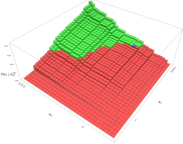
Geometrical representation.To explain the algorithms in this paper, we will use a graphical representation of the key space of which a simple case of d = 2 is depicted in Figure 2.1.
In this figure we see two subkeys k1 andk2 along the axes of the graph. The choices for them are both ordered by probability. In the x-y plane each square uniquely represents a key k1(j)|k(2i), which is the concatenation of two subkeys. For this figure we include on the z-axis the probability of each key to illustrate the gradual differences of probabilities in the space.
The blue key represents the key k∗ used in the implementation that was attacked. The green keys are those with a higher probability than k∗, the red those with a lower probability. These are respectively equal to the keys with lower and higher rank than k∗.
Fig. 2.1: A graphical representation of the key space
In the graphical representation this would mean starting at the top-left square and using the corresponding key to decipher a ciphertext (or some equivalent check that verifies the key). If this does not yield the desired results, then we try squares one by one, in order of their probabilities until one corresponding key does work. This would mean trying all the green squares, until we reach the blue square, which will decipher the ciphertext. The rank ofk∗ is then equal to the number of keys we tried.
The difficulty in deciding which key to check next is that we have to compute and store the probabilities of the keys that might be the next key. If we naively continue to enumerate the number of possibilities grows and eventually becomes too large to store. Smarter key enumeration algorithms were presented in [12] and [17]; their goal is to work through the candidate keys in the best possible way while keeping storage costs to a minimum.
3
The Rank Estimation Problem
We wish to estimate the number of keys with rank lower than a given key. To make this more explicit we first discuss the underlying problem that needs to be solved.
Probability Product Problem. Given a multiset P of multisets S containing reals in the open interval (0,1), and given p∗, compute
count(P, p∗) = X
p∈Q
S∈PS
1[p∗ < Y
s∈p s].
In this problem definition, multisets are unordered lists that can contain duplicates. They will be discussed more extensively in Section 7. The vectors p indexing the sum in the definition of the count function consist of one element from each multiset S; the count function counts the number of these vectors whose product of coefficients evaluate to a value higher than p∗. For large sets
P and S calculating count can become infeasible.
The Probability Product Problem is a generalization of the rank estimation problem. For rank estimation the multiset P consists of d subkey probability distributions S. Each distribution S is itself a multiset of probabilities for the values of each subkey, which resulted from for instance a side-channel attack. The other inputp∗ is the probability of the master keyk∗used in the implementation. The output count(P, p∗) is exactly the number of master keys that have a higher probability thank∗ in the SCA results, i.e., the rank ofk∗ minus 1. In this setting we refer to count(P, p∗) as rank(P, p∗) = rank(k∗).
Enumeration of allpwithp∗ <Q
s∈psreveals the exact value of rank(P, p
∗) but is often too slow to be feasible. The remainder of this paper considers much faster methods to determine tight lower and upper bounds for the rank function. These algorithms are explained in the context of SCA results, but the reader should keep in mind that they can also be applied to the more general form of the Probability Product Problem.
4
The Rank Estimation Algorithm (REA)
The first rank-estimation algorithm was presented by Veyrat-Charvillon, G´erard and Standaert in [18]. We explain their algorithm using the geometric represen-tation from Section 2. As before, each of the d ordered subkey attack results is represented by an axis in the d-dimensional space. Each (hyper)-square then represents a key k.
This space has the nice property that for a point (key) with coordinates (i1, . . . , id) the downwards induced box consisting of the points (i01, . . . , i0d), with
Now if we have a key k∗ of which the rank has to be estimated, we pick a key k from the space and check whether pk ≥ p∗. If this is the case, then the downwards induced box contains only keys with ranks lower than rank(k) and therefore lower than rank(k∗). If this is not the case then the upwards induced box consists of keys with rank higher than that of rank(k∗). The number of grid points in this induced box can be determined, the points removed from the space and the estimate for the rank of rank(k∗) can be updated accordingly. This process can be iterated as long as the bounds are not tight enough.
A hyperrectangle can be stored entirely by its two extreme squares. A hy-perrectangle from which one induced box has been removed can be stored as the difference of two hyperrectangles and requires storing three points. Removing more induced boxes will make the space harder and harder to store. In [18] this is solved by only storing hyperrectangles and differences of hyperrectangles. If we want to remove more we first cut the difference of two hyperrectangles into two pieces, at least one of which is a hyperrectangle. We then recursively repeat the process on the two pieces. This algorithm is summarized in Algorithm4.1.
Algorithm 4.1: Rank Estimation Algorithm (from [18])
Data: Ordered subkey distributions P ={p(ij)}1≤i≤d,1≤j≤v and probability p∗
of the used keyk∗
Result: An intervalI = [I1;I2] containing rank(P, p∗)
begin
L ← {[1;v]d} I ←[1;vd]
while L 6=∅ do
V ←maxV∈L|V|
L ← L \V
if V = hyperrectangle then
pick point inV, carve corresponding hyperrectangle fromV and updateV;L ← L ∪V
Update I
else
SplitV into V1 and V2
L ← L ∪V1∪V2
return I
implementation of DES, but for non-extreme values in AES-128 this is already infeasible. However the algorithm can be aborted before an exact rank is found and I gives bounds for rank(k∗). The longer the algorithm is run, the smaller the size of I and the better the bounds. We present tightness bounds resulting from the Rank Estimation Algorithm in Section 6.
5
Extended Rank Estimation Algorithm (EREA)
An advantage of the Rank Estimation Algorithm is that when we stop the algo-rithm we not only are left with an estimate for rank(k∗), but we also have the remaining space of keys stored. In this section we present our first result: the Extended Rank Estimation Algorithm (EREA) which derives extra information from this remaining key space by way of a statistical extension.
Statistical algorithms were briefly considered in [18] as easy but inefficient ways to estimate the rank of a key. These algorithms sample random keys and obtain an estimate for the rank by computing how many of the sampled keys have a higher posterior probability than k∗. The resulting bounds are too rough to obtain any meaningful result for the algorithms (AES-128 and LED) considered in [18].
We propose to combine REA with statistical algorithms as a post processing stage: After running REA we draw n random points from the remaining space and for each of these calculate the probability of the corresponding key k and compare it top∗. This tells us whether the drawn key has a higher or lower rank than k∗. By keeping track of the quotient of higher and lower ranked keys, we can create a (1−δ)-confidence interval for rank(k∗). Different values for δ can be chosen by the evaluator to suit his needs.
This extension is summarized in Algorithm5.1. In this algorithm we run REA for time t before stopping it and then sample n keys; B denotes the binomial distribution.
For large n the sampling converges to drawing n|V|/|L| samples from each boxV, which is also what we would expect if we were drawing uniformly from the entire remaining space. We note that the allotted sample size input is almost never the exact number of samples drawn, but serves as an indicative order size of the sample. For our implementation we included one extra step before the sampling: REA represents carved boxes as differences of two boxes which makes drawing samples from them more complicated. We solved this problem by splitting the carved boxes up into hyperrectangles.
6
Experimental results for EREA
Algorithm 5.1:Extended Rank Estimation Algorithm (EREA)(from [16])
Data: Subkey distributions P ={p(ij)}1≤i≤d,1≤j≤v, probability p∗ of the actual
key, time t, sample sizen, and confidence values δ
Result: An intervalI = [I1;I2] containing rank(P, p∗) with 100% confidence and intervals Iδ = [Iδ0;Iδ1] containing rank(P, p
∗
) with (1−δ)·100% confidence
begin
(L, I)←REA(P, p∗, t)
for V ∈ L do
Sv ←Sample sizenV =B
n,||L|V|from volumeV
S ←S
V∈LSv
Compute confidence intervals from I, S andδ’s
return I and the Iδ
determined experimentally to have rank approximately 20,24,221,227,234,239, 242,246,248, 253,257,260,266,276,280,283, 292,297,2102,2107,2112,2119,2125, 2127 and 2128. Of these keys the actual key used in the smart card during the attack was one of rank ∼ 2125. We ran the algorithms on a single core of an AMD FX-8350 Vishera 4.0GHz CPU of the Saber cluster [2].
For comparison we first ran REA on our results. To do this we used the C++ code that was published with [18]. The quality measure chosen by [18] is the difference in the log2 upper and lower bounds of the intervals obtained after a certain running time. This is the same as log2(I2/I1), i.e., it gives a measure on the ratio of the interval bounds. Figure 6.1 presents the average results over 20 executions. This figure shows the same effect for the different running times as Figure 5 in [18] but our computations take longer; this is easily explained by us using different hardware.
These running times ignore a preprocessing phase. In this phase some of the subkeys are combined to make the graphical representation lower dimensional, e.g., for AES-128 the attack uses d = 6. This increases the convergence of the algorithm to a speed where the algorithm becomes useful, but the preprocessing took us over 40 seconds for AES-128 attack results.
The graph shows that log2(I2/I1) is largest for keys with ranks around 280. This makes sense because these keys are situated in the center of the initial hyperrectangle so that the carving can never remove particularly large boxes and the algorithm needs to process several hyperrectangles, making it take more iterations. Also note that for large ranks the ratio I2/I1 is relatively small, without decreasing the interval size itself because the same ratio corresponds to a much larger difference I2−I1.
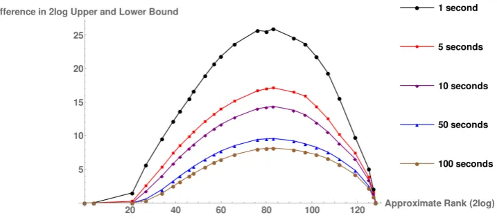
For the experiments for EREA we considered the worst case for REA, a key of rank ∼ 280. For particularly low- or high-ranked keys REA will efficiently decrease the ratio of the interval bounds so that sampling is less necessary; for keys in the range of 250 (broken) to 2100 (unbroken) the sampling is most important. We ran REA followed by the statistical sampling. The results are in Figure6.2.
Fig. 6.2: The bounds resulting from the Extended Rank Estimation Algorithm.
In this graph the black (outermost) lines display the bounds resulting from REA. These were induced from the bounds checked at t = 1,5,10,50,100, and 500 seconds. We then ran EREA, stopping with the REA part after t = 1,5,10,50, or 100 seconds. The other lines in the graph show the resulting 99.9% confidence intervals.
longer means the remaining space gets cut up into more boxes, which in turn means that we have to iterate through a longer queue of boxes when sampling. Hence, the best results are obtained by running REA for only a short time (in this example 5 or 10 seconds) and then switching over to the statistical sampling method. Better implementations of REA might shift the exact cut off but do not change the general result that sampling leads to significant time savings once the sampling range is small enough.
7
Polynomial Rank Outlining Algorithm (PRO)
This section presents our new Polynomial Rank Outlining Algorithm (PRO) that computes arbitrarily tight lower and upper bounds on key ranks.
We draw an analogy between computing the rank of a keyk∗ and computing a number-theoretic function traditionally called Ψ(x, y). By definition Ψ(x, y) is the number of y-smooth integers ≤x; here a y-smooth integer is an integer whose prime decomposition contains no primes greater than y. The analogy is easy to see: the number of y-smooth integers ≤x is the number of products
≤x of powers of primes ≤y; the rank of k∗ is the number of products >pk∗ of
subkey probabilities, i.e., the number of products<1/pk∗ of reciprocals of subkey
probabilities.
PRO is inspired by an algorithm from Bernstein [1] that computes arbitrarily tight lower and upper bounds on Ψ(x, y). The rest of this section explains how PRO works.
Ingredients of PRO. We begin by introducing the concepts used in PRO, in particular the concepts of multisets and generalized polynomials. The latter is similar to the concept of a generalized power series used in [1], but is simpler since it has only finitely many terms.
A multiset is defined as a generalization of a set. Where in a set each element can appear only once, there can be multiple instances of identical members in a multiset. There is no standard, concise and unambiguous notation for multisets. In this paper we will use the notation of a sum of multisets of 1 element. A multiset M containing the elementsa, b, b, cwill be denoted as{a}+{b}+{b}+
{c}.
As an example of a multiset, consider a subkey that has values 0,1,2,3,4 with probabilities 1/12,1/2,1/12,1/12,1/4 respectively. The multiset of probabilities is the multiset{1/12}+{1/2}+{1/12}+{1/12}+{1/4}, which is the same as the multiset {1/12}+{1/12}+{1/12}+{1/4}+{1/2}. The multiplicity of 1/12 in this multiset is 3, the number of occurrences of 1/12.
We can then also define the addition of two multisets. Let M1, M2 be two multisets, then
M1+M2 = X m1∈M1
{m1}+ X m2∈M2
{m2}
M1·M2 =
X m1∈M1,m2∈M2
{{m1}+{m2}}.
The product thus consists of multisets of size 2 with combinations of an element in M1 and an element in M2. The multiplicity of {{m1}+{m2}} in
M1 ·M2 is the product of the multiplicity of m1 in M1 and the multiplicity of
m2 in M2. The multiplication can easily be extended to the product of more multisets.
For example, consider a second subkey that has values 0,1,2 with proba-bilities 1/3,1/2,1/6 respectively. The multiset M2 of probabilities is {1/6}+
{1/3}+{1/2}. The sum M1+M2, whereM1 is the previous example {1/12}+
{1/12}+{1/12}+{1/4}+{1/2}, is{1/12}+{1/12}+{1/12}+{1/6}+{1/4}+
{1/3}+{1/2}+{1/2}. The product M1·M2 is the following multiset, where for conciseness we abbreviate 1/2 as 2 etc.:
{{12}+{6}}+{{12}+{6}}+{{12}+{6}}+{{4}+{6}}+{{2}+{6}}
+{{12}+{3}}+{{12}+{3}}+{{12}+{3}}+{{4}+{3}}+{{2}+{3}}
+{{12}+{2}}+{{12}+{2}}+{{12}+{2}}+{{4}+{2}}+{{2}+{2}}
We emphasize that order does not matter, and that this is the same multiset:
{{12}+{6}}+{{12}+{6}}+{{12}+{6}}+{{12}+{3}}+{{12}+{3}}
+{{12}+{3}}+{{12}+{2}}+{{12}+{2}}+{{12}+{2}}+{{6}+{4}}
+{{6}+{2}}+{{4}+{3}}+{{4}+{2}}+{{3}+{2}}+{{2}+{2}}.
Lastly we note that one can create multisets of multisets just like one can create sets of sets. The product of two multisets is an example of this. Given multisets
M1, . . . , Md, one can build the multiset M = Pi=1,...,d{Mi} containing those
d multisets. Note that by definition M is unordered and can contain duplicate multisets.
Ageneralized polynomialis a functionF :R→Rsuch thatF(r)6= 0 for only finitely many r ∈ R. The reader should visualize F as the sum P
r∈RF(r)xr, where x is a formal variable. Generalized polynomials are added, subtracted, and multiplied as suggested by this sum: the sum F +G of two generalized polynomials F and G is defined by (F +G)(r) = F(r) +G(r), the difference
F −G is defined by (F −G)(r) = F(r)−G(r), and the product F G is defined by (F G)(r) =P
s∈RF(s)G(r−s).
The distribution of a generalized polynomial F, denoted as distrF, is the function that maps h to P
r≤hF(r). Distributions satisfy several useful rules: (distr(−F))(h) =−(distrF)(h),
(distr(F +G))(h) = (distrF)(h) + (distrG)(h),
(distr(F G))(h) =X s∈R
Lastly, we define a partial ordering ≤ on generalized polynomials: we say thatF ≤G if (distrF)(h)≤(distrG)(h) for all h∈R. If F1, . . . , Fn, G1, . . . , Gn satisfy Fi ≤ Gi and Fi(r)≥ 0 and Gi(r) ≥0 for all i then
Qn
i=1Fi ≤ Qn
i=1Gi; see [1]. We will use this result in the next subsection.
Outlining the ranks. Recall that d is the dimension of the attack, i.e., the number of subkeys that were attacked; thatk(ij) is the jth most likely value for the ith subkey; and that p(ij) is the probability of this value.
In the Polynomial Rank Outlining Algorithm (PRO) we can simplify this notation. The ordering of the probabilities was important for REA, because of its use of a geometrical representation. With PRO we do not need ordered probabilities and therefore we will represent the probabilities resulting from the SCA as multisets. More specifically, as in Section 3, we assume that an attack on d independent subkeys results in a multiset P of d multisets S of subkey probability distributions. Given the probability p∗ of the implemented key k∗
we want to bound the function:
rank(P, p∗) = X
p∈Q
S∈PS
1[p∗ < Y
s∈p s].
PRO separately creates lower and upper bounds for this function. We will explain how to calculate the upper bound; the lower bound is constructed simi-larly. We first define the following functions on probabilities. Letα be a positive real number; we will obtain tighter bounds by increasing α, so we call α the “accuracy parameter”. The function ˜· : (0,1)→R is defined as:
˜
p=α·log2(1/p),
and the function · : (0,1)→Zis defined as:
p=bα·log2(1/p)c=bpc˜ .
We now have the nice property that if the probability p is the product of the subkey probabilities in p∈Q
S∈PS then ˜
p=α·log2(1/p)≥ bα·log2(1/p)c ≥X
s∈p
bα·log2(1/s)c. (1)
With these definitions in mind we define a generalized polynomialFP as follows:
FP = X p∈J
xp˜= Y S∈P
X s∈S
x˜s,
where J = P
p∈Q
S∈PS{
Q
s∈ps} is the multiset of all master key probabilities.
In other words, FP is a generalized polynomial which contains one term xp˜ for each master key with probability p.
smaller than ˜p∗: Using the notation introduced above, rank(k∗) = rank(P, p∗) = distr(FP)(˜p∗). We do not mean to suggest that counting these terms one by one is feasible: for example, for a key of average rank in AES-128, if we neglect equal exponents, this would mean counting ∼2127 terms, which is infeasible. To solve this problem we will create a generalized polynomialGmeeting three goals: first,
G has far fewer terms than F; second, G≥F; third, the gap between G and F
becomes arbitrarily small asα increases. We define G as follows:
GP(x) = Y S∈P
X s∈S
xs.
Note that this consists only of integer powers ofx. Now, because of (1),P
s∈Sxs ≥ P
s∈Sx ˜ s, so G
P ≥FP.
In particular, (distrGP)(˜p∗) ≥ (distrFP)(˜p∗) = rank(P, p∗). We have thus created an upper bound for the rank ofk∗. Similarly, if we replace the function ·
by a function,· : (0,1)→Zwithp=dpe˜ , we obtain a lower bound for rank(k∗). How tight these bounds are, will be discussed below.
PRO is stated in Algorithm 7.1.
Algorithm 7.1: Polynomial Rank Outlining Algorithm (PRO)
Data: Subkey distributions P, the key probability p∗ and an accuracy parameterα
Result: An intervalI = [I1;I2] containing rank(P, p∗)
begin
GP(x)←QS∈PPp∈Sxp
HP(x)←QS∈PPp∈Sxp
I1←distrHP(˜p∗)
I2←distrGP(˜p∗)
return I
Margin of error. Now that we have shown that we can create a bound, we can analyze how tight it is. The size of the interval resulting from Algorithm7.1
is directly dependent on α. The larger α is, the fewer distinct values s and s, where s∈ S and S ∈ P, will evaluate to the same integer and the more distinct monomials G and H will have. We will show how to derive an upper bound for the upper bound. A lower bound for the lower bound is derived analogously. Let, for each S ∈ P,
S = min
s∈S(s/s˜), (2)
then we can define:
E = X
S∈P (
X s∈S
{S ·˜s} )
Then, because it holds that
∀S ∈ P :∀s∈ S :S ·s˜≤s, it follows that
Y E∈E
X e∈E
xe≥ Y
S∈P X s∈S
xs.
Letp∗ =Q
s∈ps for somep∈
Q
S∈PS, then we definep∗ = Q
s∈ps
S, where the S are such that s∈ S. Then distr(FP)(˜p∗)≥distr(GP)(˜p∗), which means that we have an upper bound for the rank upper bound. Similarly we can replace the min in Equation2 by a max and the functions · in Equations 2and 3by ·, to find a lower bound of distr(FP)(˜p∗) for the rank lower bound.
Computing this upper bound for the upper bound is expensive. However, we can derive information from this upper bound without actually computing it: we simply compute the values S. We see that these values are directly dependent on the accuracy parameter α.
lim
α→∞S = limα→∞mins∈S(s/s˜) = limα→∞mins∈S
bα·log2(1/s)c α·log2(1/s) = 1.
The error margin does not give an indication of how many keys the interval contains, but it does give an indication of what probability the keys in the interval have. For the p∗ defined above the rank interval computed by PRO will at most contain all ranks of the keys with probabilities between p∗ and p∗.
We will see in Section 8that in practice the bounds of the interval are closer to distr(FP(x)) than to the maximum error bounds.
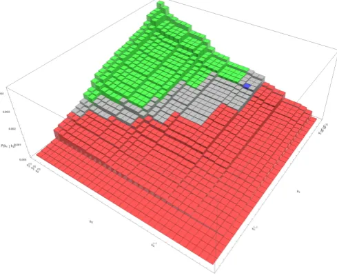
PRO in the graphical representation.In Section4we explained REA using the geometrical representation seen in Figure2.1. We can use this 2-dimensional representation to visualize the bounds produced by PRO. We again take the squares representing the keys but now we color them a bit differently. The blue key k∗ with probability p∗ still represents the key used in the attack. The red area are the keysk for which it holds thatbαlog2(1/s1)c+bαlog2(1/s2)c>p˜∗, wheres1 ands2 are the probabilities of the subkeys used. The green area are the keys k for which it holds that dαlog2(1/s1)e+dαlog2(1/s2)e < p˜∗. The grey area consists of the remaining keys. An example of this is shown in Figure 7.2. To give an upper bound for the rank of k∗ we want to count the number of keys in the green and grey areas. This is however infeasible for high key ranks, so we simplify the space to speed up this process. By combining subkeys that are close to each other, where the definition of close is dependent on α, we can count boxes filled with a known number of keys. In Figure 7.3 we see this for our previous example, using the value α= 4.
Fig. 7.2: Geometrical representation of the key space with the grey area.
In this geometrical representation we also see the distance between the lower and upper bound as the grey area. This is the area we estimate with the error
. The larger α is, the smaller the grey area is and the tighter our bounds are.
8
Experimental results for PRO
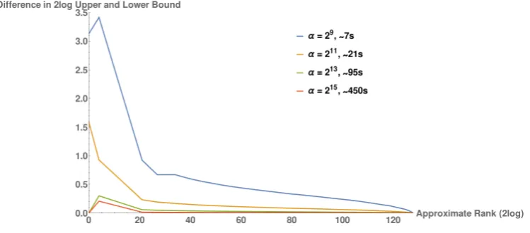
We ran PRO for the same attack results and keys considered in Section 6using an implementation in Sage. In Figure 8.1 we see the resulting log-difference in bounds for some values ofα, as well as the time it took.
The time it takes to calculate the bounds scales with the accuracy parameter. The log-difference between the lower and upper bound seems to decrease by approximately the factor by which we increase the accuracy parameter, with the exception of the very low ranks. This is similar to the REA results where the keys with low rank also behaved more erratically. The slight overhead for the other ranks is mostly the time to count the coefficients of the polynomial.
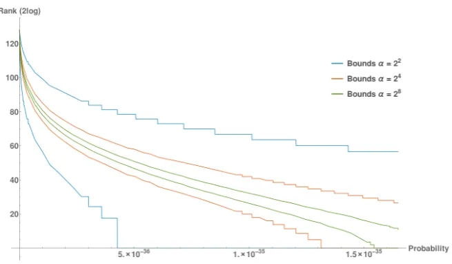
We can adapt Algorithm 7.1 a bit to give a different representation of the results by inputing the smallest probability master key produced by the side-channel attack for p∗ and computing G and H not only for ˜p∗, but also for all values of p. We can then convert these integers back to ranges of probabilities. For our experiments with α = 4,16,64 this resulted in Figure 8.2.
We see that the higher the value ofα, the smoother the graphs are. A higher
αmeans fewer probabilities fall into the exponent of one term of the polynomial. PRO’s ability to create such a graph for all probabilities is unmatched by REA. REA can only do evaluations for one key at a time.
Fig. 7.3: Simplified geometrical representation using α= 4.
Fig. 8.1: The difference between the log2 upper and lower bound for different values of α.
accuracy parameter of α = 29, which means a running time of only 7 seconds, all our tested keys had a log distance below 4.
The shape of the graph is also a major difference. While the most ‘difficult’ keys for REA were the ones with rank∼280, for the PRO algorithm the estimate is the least accurate (in the log distance) for the lowest ranks. This is explained by the methodologies of the algorithms. As stated before, for REA the most difficult ranks are those in the middle of the graphical representation. For PRO the lower ranked keys are represented by just a few terms of the power series. We might need to choose a rather high value for α for these keys to be spread across different polynomial terms which improves the bounds.
Fig. 8.2: Graphical representation of all side-channel results.
phase however the space starts to consist of more and more smaller and smaller boxes. This means that less can be cut after each iteration of the algorithm. In PRO the desire for a more accurate bound translates into choosing a higher accuracy parameter. If we assume uniformly spread probabilities and we double
α then the grey area in Figure7.2, which consists of keys bounded by floors and ceilings of αlog2(1/pi), will decrease as the grey boxes get split up and change color. Of course the keys are not uniformly spread and the convergence will thus not be constant, but it will not stagnate as much as for the rank estimation algorithm.
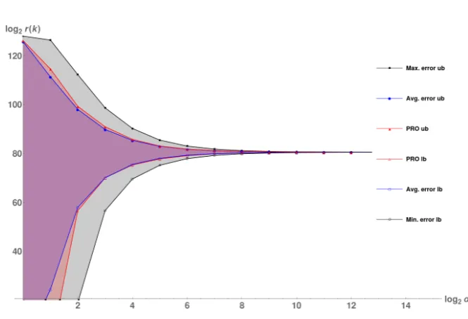
We move on to experiments for the error bound of our bounds. For a key of rank ∼280 the results are shown in Figure 8.3.
We see that using the error from Equation (3) results in pretty wide margins for the bounds found by PRO. We therefore reran our test replacing the maximal and minimal error in the calculations by the average error. This resulted in a much better approximation of the bounds, but we can see these are no longer strict lower and upper bounds for the interval resulting from PRO. It might however be a better indication for an evaluator of which accuracy parameter α
he should take to reduce his running time.
We can now compare the REA results to the results of the new algorithms. To this end we have graphed comparable timescales for all the algorithms in Figure8.4.
These results imply that PRO outperforms REA for most of the possible ranks. For the ranks where REA works better, it is unlikely that one would use an algorithm to derive the rank in the first place, because it will be clear that the implementation is broken (the subkeys of k∗ all have very high probability and the key can be enumerated within a few seconds).
con-Fig. 8.3: The estimated error versus the actual bound for a key with rank(k)∼
280. Here lb means the lower bound and ub the upperbound.
Fig. 8.4: The log difference between the bounds of REA (black), EREA (red) and PRO (blue). Left: Runtimes with sub-10-second performance; ∼ 7s. for PRO withα = 29), ∼8s. for EREA with 5s. REA/220 samples and 10s. for the REA. Right: Runtimes with sub-2-minute performance; ∼ 106s. for PRO with
α= 213),∼108s. for EREA with 100s. REA/28 samples and 106s. for the REA.
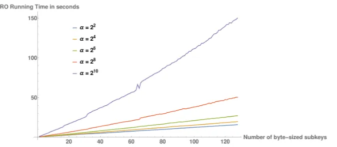
struct the bounds for the key with the highest rank. This is the key for which the most work needs to be done by PRO, and as a side effect produces bounds for all lower-ranked keys. The resulting time for PRO is shown in Figure 8.5. The tightness of the PRO bounds is shown in Figures8.6and Figure 8.7for keys of two different ranks, as discussed below.
lower-Fig. 8.5: The number of attacked subkeys versus the running time of PRO for several values of α.
precision approximations to the coefficients, either accepting approximations as output or using interval arithmetic to obtain rigorous bounds; second, use power-series logarithms as in [1].) It is not difficult to extrapolate the running times for larger attacks, although we observed some slowdowns for very large 2048-bit keys (256 subkeys) withα = 213 because Sage ran out of RAM and began swapping. Contrary to REA, PRO cannot output any result until the algorithm is run completely. The accuracy parameter α should thus also be limited to feasible running times.
Fig. 8.6: For several values of α: The number of attacked subkeys versus the bounds produced by PRO for the master key of rank 1.
Fig. 8.7: For several values of α: The number of attacked subkeys versus the bounds produced by PRO for the master key where each subkey has rank 5.
distance seems to require quadruplingα in Figure 8.6 but merely doublingα in Figure8.7.
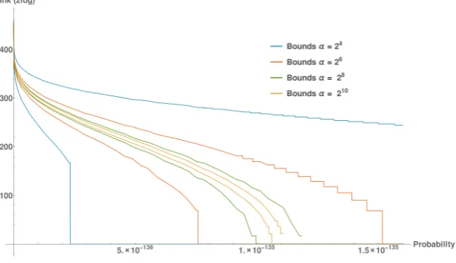
Figure 8.8 shows the lower and upper bounds for all key ranks for α = 24,
α = 26, α = 28, and α = 210 for 64 byte-sized subkeys (and thus a 512-bit master key). Computing all of these bounds took less than 30 seconds, less than the time needed for preprocessing REA on just 16 byte-sized subkeys.
Fig. 8.8: Graphical representation of uniform random side-channel results on a master key of 64 subkeys.
the bounds resulting from measurement results in Figure 8.2 to the distance in bounds produced by uniform subkey distributions in Figure 8.6, we see that bounds for higher ranked keys and on non-uniformly distributed subkeys are even tighter.
9
Comparison
There are some advantages to REA. For extremely small ranks the algorithm performs better than PRO, even if we take preprocessing time into account. On the other hand, in side-channel attacks in which the result is so significant, the exact rank will also be clear from the results and there is no need for a rank estimation. For those small ranks we can enumerate to the key in under a second and an evaluator should in any case first check whether p∗ is overwhelmingly large.
Another advantage of REA is the ability to interrupt the algorithm to get a result and even continue an estimation at a later time. If the algorithm has been run and the remaining space has been stored, then continuing the algorithm when a better estimate is necessary is easily done. This also holds for taking more samples in EREA. If during an evaluation PRO is used and a better estimate is wanted at a later time, the algorithm needs to be rerun with a higher α. Also, if PRO is terminated before finishing, then there are no results. On the other hand, if the cost of continuing REA is more than the cost of running PRO from scratch, then this is obviously not an advantage for REA.
EREA (Section5) is also a reason to pick REA over PRO. EREA outperforms PRO for quick estimates (and also for very small key ranks), at least if we ignore the initial preprocessing: Using as few as 28samples and a 99.9% confidence level, the estimate can be improved in very little time. Convergence of sampling has a very fast initial convergence and it does not have the overhead of operations like multiplication of polynomials. We see this in Figure8.4. In this case however the interval of which we know with 100% certainty that it contains the rank is very large. We have not found a way to do similar sampling for PRO.
PRO has larger advantages. For one it does not need the combining of dimen-sions to get good results. This preprocessing for REA took us over 40 seconds, a time in which PRO already gives a good result. Of course, EREA needs the same preprocessing as REA.
AES-128. This matches theoretical expectations. Probabilities in AES-256 will on average be the squares of probabilities of AES-128 keys. This means that the degrees ofG andH approximately double. This causes the doubling of the time needed to calculate G and H and the number of keys represented by each term to be squared.
The last advantage of the PRO method we wish to re-iterate is the remaining space or grey area. With the rank estimation algorithm this can have a lot of shapes, depending on the way the cutting points are chosen. This also means that one cannot say anything certain about the probabilities of the keys remaining in the interval. With PRO, as we saw in Section 7, the keys that lie within the bounds have certain properties. Using the error margin from Section 7 we can even give concrete probabilities which certainly lie outside of the interval. This algorithm thus gives a lot better indication of the remaining space. As we saw in Figure 8.2 we can adapt Algorithm7.1 to handle all possible keys at once in a black-box fashion, allowing the key holder to quantify the security of a strong secret key without disclosing the key to the evaluator.
References
1. Daniel J. Bernstein. Arbitrarily tight bounds on the distribution of smooth integers. In M. A. Bennett, B. C. Berndt, N. Boston, H. G. Diamond, A. J. Hildebrand, and W. Philipp, editors, Number theory for the millennium. I: papers from the conference held at the University of Illinois at Urbana-Champaign, Urbana, IL, May 21–26, 2000, pages 49–66. A. K. Peters, 2002. http://cr.yp.to/papers. html#psi.
2. Daniel J. Bernstein. The Saber cluster, 2014. http://blog.cr.yp.to/ 20140602-saber.html.
3. Eric Brier, Christophe Clavier, and Francis Olivier. Correlation power analysis with a leakage model. In Marc Joye and Jean-Jacques Quisquater, editors, CHES 2004, volume 3156 of Lecture Notes in Computer Science, pages 16–29. Springer, 2004.
4. Suresh Chari, Josyula R. Rao, and Pankaj Rohatgi. Template attacks. In Burton S. Kaliski Jr., C¸ etin Kaya Ko¸c, and Christof Paar, editors, CHES 2002, volume 2523 of Lecture Notes in Computer Science, pages 13–28. Springer, 2002.
5. Markus Dichtl. A new method of black box power analysis and a fast algorithm for optimal key search. J. Cryptographic Engineering, 1(4):255–264, 2011.
6. Cezary Glowacz, Vincent Grosso, Romain Poussier, Joachim Schueth, and Fran¸cois-Xavier Standaert. Simpler and more efficient rank estimation for side-channel security assessment. Cryptology ePrint Archive, 2014. http://eprint. iacr.org/2014/920.
7. Pascal Junod and Serge Vaudenay. Optimal key ranking procedures in a statistical cryptanalysis. In Thomas Johansson, editor, FSE 2003, volume 2887 of Lecture Notes in Computer Science, pages 235–246. Springer, 2003.
8. Paul C. Kocher, Joshua Jaffe, and Benjamin Jun. Differential power analysis. In Michael J. Wiener, editor, Crypto ’99, volume 1666 ofLecture Notes in Computer Science, pages 388–397. Springer, 1999.
10. Mitsuru Matsui. Linear cryptanalysis method for DES cipher. In Eurocrypt ’93, pages 386–397. Springer, 1994.
11. National Institute of Science and Technology (NIST). Announcing the Advanced Encryption Standard (AES), 2001. http://csrc.nist.gov/publications/fips/ fips197/fips-197.pdf.
12. Jing Pan, Jasper G. J. van Woudenberg, Jerry den Hartog, and Marc F. Witteman. Improving DPA by peak distribution analysis. In Alex Biryukov, Guang Gong, and Douglas R. Stinson, editors,SAC 2010, volume 6544 ofLecture Notes in Computer Science, pages 241–261. Springer, 2010.
13. Ali Aydin Sel¸cuk. On probability of success in linear and differential cryptanalysis.
J. Cryptology, 21(1):131–147, 2008.
14. Fran¸cois-Xavier Standaert, Tal Malkin, and Moti Yung. A unified framework for the analysis of side-channel key recovery attacks. In Antoine Joux, editor, Euro-crypt 2009, volume 5479 of Lecture Notes in Computer Science, pages 443–461. Springer, 2009.
15. Adrian Thillard, Emmanuel Prouff, and Thomas Roche. Success through confi-dence: Evaluating the effectiveness of a side-channel attack. In Guido Bertoni and Jean-S´ebastien Coron, editors, CHES 2013, volume 8086 ofLecture Notes in Computer Science, pages 21–36. Springer, 2013.
16. Christine van Vredendaal. Rank estimation methods in side channel attacks. Mas-ter’s thesis, Eindhoven University of Technology, 2014. http://scarecryptow. org/publications/thesis.html.
17. Nicolas Veyrat-Charvillon, Benoˆıt G´erard, Mathieu Renauld, and Fran¸cois-Xavier Standaert. An optimal key enumeration algorithm and its application to side-channel attacks. In Lars R. Knudsen and Huapeng Wu, editors,SAC 2012, volume 7707 of Lecture Notes in Computer Science, pages 390–406. Springer, 2012. 18. Nicolas Veyrat-Charvillon, Benoˆıt G´erard, and Fran¸cois-Xavier Standaert. Security
evaluations beyond computing power. In Thomas Johansson and Phong Q. Nguyen, editors,Eurocrypt 2013, volume 7881 ofLecture Notes in Computer Science, pages 126–141. Springer, 2013.