Absorption Capacity, Structural Similarity and Embodied Technology Spillovers in a 'Macro' Model: An Implementation Within the GTAP Framework

Full text

(1)CENTRE of POLICY STUDIESand the IMPACT PROJECT. Eleventh Floor Menzies Building PO Box 11E, Monash University Wellington Road CLAYTON Vic 3800 AUSTRALIA Telephone: (03) 9905 2398, (03) 9905 5112. from overseas: 61 3 9905 5112 or 61 3 9905 2398. Fax: (03) 9905 2426 e-mail. 61 3 9905 2426 [email protected]. web site. http://www.monash.edu.au/policy/. ABSORPTION CAPACITY, STRUCTURAL SIMILARITY AND EMBODIED TECHNOLOGY SPILLOVERS IN A ‘MACRO’ MODEL: AN IMPLEMENTATION WITHIN THE GTAP FRAMEWORK by. Gouranga Gopal DAS and. Alan A. POWELL Centre of Policy Studies, Monash University. Preliminary Working Paper No. IP-77 December 2000. ISSN 1 031 9034. ISBN 0 7326 1528 3. The Centre of Policy Studies (COPS) is a research centre at Monash University devoted to quantitative analysis of issues relevant to Australian economic policy..

(2) ABSTRACT In this paper, all technology transfers are embodied in trade flows within a three-region, one-traded-commodity version of the GTAP model. Exogenous Hicks-Neutral technical progress in one region can have uneven impacts on productivity elsewhere. Why? Destination regions’ ability to harness new technology depends on their absorptive capacity and on the structural congruence of the source and destination. Together with trade volume, these two factors determine the recipient’s spillover coefficient (which measures its success in capturing foreign technology). Armington competition between the outputs of the three economies and shifts in their terms of trade loom large in the general equilibrium adjustment. JEL Classification: D58, F11, F41, O49.. i.

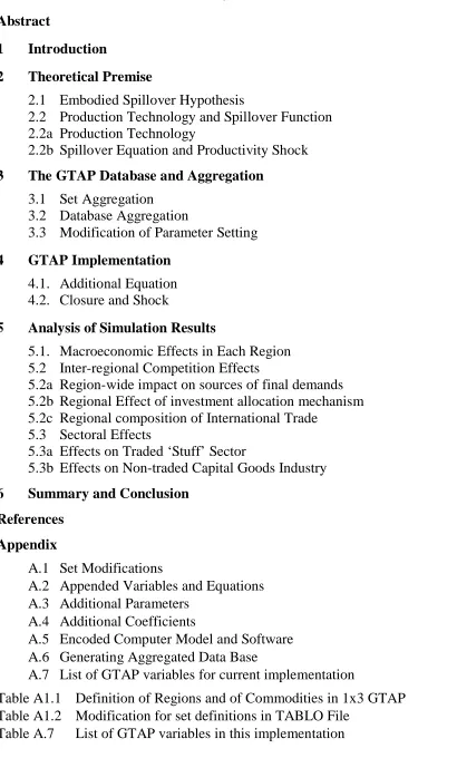
(3) CONTENTS Abstract. i. 1. Introduction. 1. 2. Theoretical Premise. 2. 2.1 2.2 2.2a 2.2b. 2 4 4 5. 3. 4. 5. 6. Embodied Spillover Hypothesis Production Technology and Spillover Function Production Technology Spillover Equation and Productivity Shock. The GTAP Database and Aggregation. 8. 3.1 Set Aggregation 3.2 Database Aggregation 3.3 Modification of Parameter Setting. 8 9 9. GTAP Implementation. 10. 4.1. Additional Equation 4.2. Closure and Shock. 10 11. Analysis of Simulation Results. 12. 5.1. 5.2 5.2a 5.2b 5.2c 5.3 5.3a 5.3b. 12 16 18 23 27 32 32 33. Macroeconomic Effects in Each Region Inter-regional Competition Effects Region-wide impact on sources of final demands Regional Effect of investment allocation mechanism Regional composition of International Trade Sectoral Effects Effects on Traded ‘Stuff’ Sector Effects on Non-traded Capital Goods Industry. Summary and Conclusion. 35. References. 37. Appendix. 39. A.1 A.2 A.3 A.4 A.5 A.6 A.7. Set Modifications Appended Variables and Equations Additional Parameters Additional Coefficients Encoded Computer Model and Software Generating Aggregated Data Base List of GTAP variables for current implementation. Table A1.1 Definition of Regions and of Commodities in 1x3 GTAP Table A1.2 Modification for set definitions in TABLO File Table A.7 List of GTAP variables in this implementation ii. 39 41 45 46 47 48 49 40 41 50.

(4) LIST OF TABLES Table 3.1.1 List of sets and their elements in 1x3 GTAP. 9. Table 3.3.1 Value of elasticities of substitution parameters. 10. Table 4.1.1 Additional equation in the TABLO source file for technology spillover. 11. Table 5.1.1. Simulated regional effects of technological change in the USA on selected macroeconomic variables. 13. Table 5.1.2 Values of embodiment-index, spillover coefficient and capture-parameter. 15. Table 5.2.1 Simulated regional effects on sources of final demand. 17. Table 5.2.2 Simulated effects on nominal regional income. 18. Table 5.2.3 Budget shares of each income use category and incdeflator. 20. Table 5.2.4 Component-wise effects on pgdp. 22. Table 5.2.5 Simulated effects on rate of returns and base-period values of some coefficients. 23. Table 5.2.6a Base-case values of Gross Saving and Gross Investment. 25. Table 5.2.6b Post-shock values of Gross Saving and Gross Investment. 25. Table 5.2.7 Decomposition of percentage changes in regional TOT. 29. Table 5.2.8 Simulated effects on bilateral export sales. 32. Table 5.3.1 Simulated regional effects of technology shock on Stuff. 33. Table 5.3.2 Simulated regional effects on capital goods industry. 34. FIGURES Figure 1. Production structure for region ‘r’ in the one-commodity, three-region version of GTAP. 5. Figure 2. Flow chart for the transmission mechanism in the model. 7. Figure 3. Flow chart showing the principal pathways behind the results. iii. 14.

(5) ABSORPTION CAPACITY, STRUCTURAL SIMILARITY AND EMBODIED TECHNOLOGY SPILLOVERS IN A ‘MACRO’ MODEL: AN IMPLEMENTATION WITHIN THE GTAP FRAMEWORK Gouranga Gopal DAS and. Alan A. POWELL Monash University. 1. Introduction We implement embodied knowledge spillovers in a highly aggregated version of the GTAP model — that is, a one-traded-commodity, three-region version of GTAP.1 At first sight it may seem surprising that a macro (onetraded commodity) model is used for this purpose. GTAP, like many CGE models, adopts Armington’s (1969) treatment of commodity substitution, so that even if all regions produce the same generic commodity, the substitution elasticity between that commodity produced in region A and the “same” commodity produced in region B, is not infinite. Thus, even in a onecommodity version of GTAP the ‘Law of One Price’ does not hold. Working at the one-commodity level has the advantage of concentrating on interregional competition in the goods market without having to deal with the large amount of detail entailed in keeping track also of inter-generic commodity substitution. We aggregate the GTAP database to a one-commodity and threeregion (USA, EU, and ROW) database. The generic commodity that is traded internationally will be called Stuff. Each region produces one tradable good (its own type of Stuff) and one non-tradable (its own Capital Goods). It is necessary to include a non-tradable in each region because GTAP specifies that capital formation is supplied completely by a domestic industry which does not export. Note, however, that the domestic capital goods industry in any country merely assembles a bundle of traded goods (which include foreign tradables). Consumers absorb Stuff produced at home, as well as the two imported varieties. We consider a Hicks-Neutral general total factor productivity (TFP) shock in the Stuff sector originating in one of the three regions, viz. the USA.. 1. Various aggregations of the data are available, and in this paper a 3×3 aggregation of the database is the starting point from which a further aggregation is implemented to produce a three region macro model.. 1.

(6) Such a TFP shock is general output-augmenting by nature. Its impact on productivity in the destinations is studied via an embodiment index, an absorption capacity index, and a structural similarity index. Sections 2 and 3 describe the theoretical premise and the database corresponding to our aggregation respectively. Section 4 documents the GTAP implementation, the closure and the perturbation introduced into the system. Section 5 reports and explains the simulation results. Section 6 concludes.. 2. Theoretical Premise 2.1 Embodied Spillover Hypothesis. 2. As has been argued elsewhere, growth and development of the LDCs depend not only on the extent and nature of the foreign technology which is available to them via participation in international trade in goods and services, but also on their capabilities for effectively absorbing the diffused state of the art. Current state-of-the-art technologies created by concerted research efforts are embodied in the commodities produced using the newly created ideas. The knowledge capital generated at the sources of inventions spills over to the destinations through bilateral trade linkages. This is the embodiment hypothesis: technical knowledge flows through traded goods. Note that the creation (as distinct from the transmission) of knowledge capital is beyond the scope of this paper. The adaptability and local useability of the diffused technologies depends on the Absorptive Capacity (AC) [Cohen and Levinthal3 (1989, 1990)] of the destinations and the Structural Similarity (SS) [Hayami and Ruttan (1985)] between the trading nations. In the literature, the importance of SS has been discussed especially in the context of agriculture. Here in a single-sector model with one trading sector per region, this focus is not valid. However, the maximum potential for productivity enhancement attainable with a given stock of ideas can be achieved only if both AC and SS are high.4 2. 3. 4. Our approach is more modest than the approach by Eaton and Kortum (1994, 1996a & b) [henceforth, EK], Grossman and Helpman (1991a & b), Jones (1995). All of these dynamic general equilibrium models have considered the possible interlinkages between invention, technology diffusion, growth and productivity. Eaton and Kortum have developed an empirical dynamic general equilibrium model of technology-diffusion based on a “quality-ladder” approach in which, à la Grossman and Helpman (1991a), concerted R&D effort improves the quality of the inputs over a production spectrum in continuum and this quality improvement embodied in the inputs is transmitted via the final products. Each input is produced with a conventional Cobb-Douglas, Constant Returns to Scale (CRTS) production technology where this quality-adjusted inputs are used to produce the final, traded product in a continuous analogue of the Cobb-Douglas, CRTS production function. Better quality inputs embodying the latest ideas always replace the ‘state-of-the-art’ currently in practice. To the best of our knowledge, the role of such factors in assimilating the foreign technology was first emphasised in the literarure by Cohen and Levinthal. Based on their notion of absorption capacity and its importance, some authors like Keller (1997), Nelson (1990), to name a few, have extended the discussion initiated by them. This aspect of “effective absorption” has not been studied by the authors cited above in footnote 2.. 2.

(7) Van Meijl and Van Tongeren (MT) (1997) related productivity growth rates of countries through international trade linkages and associated embodied knowledge-spillovers. In their model, AC is constructed as a binary (source- and destination-specific) index of human-capital-induced absorption capacity of Country A vis-à-vis Country B. They also use a binary index for SS. It is based on the similarity of factor proportions in the two regions (but unlike AC, SS is symmetric). These two indexes conjointly determine the ‘productive efficiency’ parameter for effective assimilation of the technology by the recipient countries.5 Our model differs in several details. First, we restrict ourselves to a one-sector (tradable Stuff) technology for production. 6 Stuff is produced in a world divided into three regions. Like “ectoplasm” in the one-sector neoclassical growth model, Stuff is easily transmutable from consumable to investment goods. Second, unlike MT where AC is a binary index involving both source and destination, we make the AC factor destination specific only. The SS factor retains its binary affix, though. Third, as will become evident below, we have modified MT’s 'embodied spillover function’. We now justify the rationale behind the latter two modifications (the reason behind aggregation of goods into a macro model has been given in the Introduction). It is argued that domestic useability of the transmitted foreign technology depends mainly on the recipient’s capability to identify, procure and utilise the diffused technology. This simplification reflects our desire to keep the model simple by concentrating on first-order effects. It seems likely that if region C is good at absorbing technology from region A, it will be equally good at absorbing technology from another region B which (from C’s point of view) is structurally similar to A. Thus, the AC factor is made destination-specific only (unlike in MT where they carry both source and destination affixes). The necessary modifications made in the basic spillover equation of MT are rationalised in the next section.. 5. 6. It is worthwhile to mention here that AC depends not only on Human Capital alone, but also on a constellation of factors such as Infrastructural Facilities, Learning Effects, and Own R&D in the recipients. However, we have not considered these factors while defining AC in our model. These are on our research agenda. The second commodity produced in each region (Capital Goods, CGDS) is produced according to a ‘technology’ which merely assembles a bundle of Stuff from the three regions. However, it is a ‘fictitious’ industry.. 3.

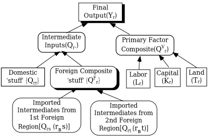
(8) 2.2 Production Technology and Spillover Function 2.2a Production Technology The production technology tree in the GTAP model uses a nested production function. Here we specialize the notation for use with the one-tradedcommodity version. At the top level, a composite output Yr is produced in region r with a Leontief fixed proportion technology using intermediate inputs Qr. and a primary input composite QVr.. Qr. is intermediate input demand for Armington composite Stuff by any region r. Each Qr. is produced in a CES production nest using domestic Stuff and a composite of foreign Stuff distinguished by country of origin (using the Armington assumption). Thus, we can write the CES production function for the intermediate input nest as -β -1/β D D F -β Qr.= Ar {δ r(Qrr) r. + (1-δ r)(Q r) r.} r.. (2.1a). where r is the region using the domestically sourced tradable Stuff Qrr and F D the foreign inputs composite of Stuff Q r. δ r is the distribution parameter (a positive fraction). β r. ≠ −1 is the substitution parameter. The superscripts D and F are used to identify domestic and foreign components respectively. The substitution elasticity between domestic and foreign Stuff is [1/(1+β r.)]. For notational convenience, in Qrs the first subscript refers to the using region and the second one refers to the foreign source of Stuff. For example, let the three regions in our implementation be A, B and C so that r,s∈{A, B, C}. Then, if r = C is the using region, and s = B or A, Qrr= QCC is the domestically sourced Stuff in C while QCA and QCB are Stuff imported by C from B and A respectively. F. Q r is produced in region r using the Stuff imported from other regions, say, s and t. Let Qrs and Qrt be respectively the intermediate input demand for Stuff from s and t by using region r. This leads us to write the F CES production nest for Q r as below: F. F. F. Q r = A r {δ r(Qrs). -β rF. F. +(1-δ r)(Qrt). -β. rF}-1/β rF. (2.1b). F. where s,t≠r; s≠t. δ r is the distribution parameter associated with this production nest. The elasticity of substitution in r between imported Stuffs is [1/(1+β rF)]. If β r.=β rF, (2.1b) is equivalent to writing Qr. as a CES function in Stuff from all three sources. V. Primary factor composite Q r is produced combining the primary f factors land (T), labor (L), and capital (K). Q r is the demand for primary factor f in region r where f∈{L, K, T}. The production technology is CES as given below: Q r = A r {Σf δVrf (Q r) r} V. V. f -ρ. -1/ρr. (2.2). where the δ rf are distribution parameters (positive fractions) (with Σf δ rf ≡ 1, ∀r) and ρr is the substitution parameter. The substitution elasticity V. V. 4.

(9) between primary factors in region r is [1/(1+ρr)]. In the above equations, Ar, F V A r and A r are technical progress parameters. V. Qr. and Q r are combined using a fixed proportion technology with no scope for substitution between intermediate inputs and the primary factors. However, as seen above, there is scope for substitution between domestic and imported varieties of Stuff, as there is between L, K and T. At the top level the (Leontief) production function is: O. V. Yr = [AO]r min { A rQr. , Q r}. (2.3). O A r. where Yr is the flow of final output and is an intermediate-inputaugmenting technical change parameter. [AO]r is the Hicks-Neutral Technical Progress (HNTP) parameter. The entire production tree for this model is depicted in Figure1.. Final Output(Yr) Intermediate Inputs(Qr.). Domestic ‘stuff’ {Qrr}. Foreign Composite ‘stuff’ {QFr}. Imported Intermediates from 1st Foreign Region[Qrs (r≠s)]. Figure 1:. Primary Factor Composite(QVr). Labor. (Lr). Capital. Land. (Kr). (Tr). Imported Intermediates from 2nd Foreign Region[Qrt (r≠t)]. Production structure for region r in the one-commodity, three- region version of GTAP. 2.2b Spillover Equation and Productivity Shock The spillover hypothesis (as documented in Section 2.1 above) is captured by a technology-transmission equation incorporating destination-specific AC and source- and destination-specific SS. Exports from source r to destination s determine an embodiment index Ers. The latter, together with ACs and SSrs determine the value of a spillover coefficient γs(Ers, ACs, SSrs) via the spillover function γs.. 5.

(10) The details of this chain are now explained, starting at the top. Note that there is only one source of exogenous technological improvement in the current treatment, so that r is unique.7 Stuff produced using the improved technology embodies this technological improvement. Exports of Stuff from r to the trade partners s transmit these embodied technological advances but do not necessarily lead to enhancement of productivity in the recipient sectors of the client countries unless they are utilized as an input to production. We define an embodiment index Ers (where 0 ≤ E rs ≤ 1 ) that is proportional to the amount of embodied knowledge received via bilateral trade linkages between r and s so that Ers= Xrs/Ys. (2.4). where Xrs is the bilateral exports of Stuff from source r to the clients s and Ys is the domestic production of Stuff in s. Thus Ers measures the amount of embodied knowledge obtained via bilateral exports from r to s per unit of output of Stuff produced in client s.8 The recipient-specific AC-index ACs (where 0 ≤ ACs ≤ 1) and the binary structural similarity index SSrs (where 0 ≤ SSrs ≤ 1) interactively determine a capture parameter θs measuring the efficiency with which the knowledge embodied in bilateral trade flows from source r is captured by the recipients s:9 θs=ACs.SSrs. (2.5). The productivity level realised from the potential streams of latest technology is dependent on θs∈[0,1] with θs=1 implying full realisation of the foreign technology-induced productivity improvement. θs and Ers jointly determine the value of the spillover coefficient γs(Ers, θs) for the destination s. γs(.) is a strictly concave function of Ers with the properties that γs(0) = 0; γs(1) = 1; γ s′ = (1−θs)Ers. −θ s. > 0; γ ′′s = −θs(1−θs)/Ers. 1+θs. < 0;. where primes indicate the first (′) and the second (′′) derivatives with respect to Ers.. 7 8. 9. An implication of the uniqueness of r is that equations carrying an r-subscripted variable on the right do not necessarily require an r subscript to appear on the left. However, it is to be noted that in MT, Ers is defined as the ratio of bilateral trade flows (Xrs) from r to s in any final product sector and total bilateral trade flows (∑sXrs) to all destinations s from the source r. This ratio shows the spillover to the recipients as a proportion of aggregate ‘global’ spillovers from source to the client countries. This seems to neglect the public good character of knowledge capital. We have modified this definition as described in the text. It has already been mentioned in footnote 5 that AC depends on several factors which we set aside in our present discussion. Depending on those factors, AC could be ‘endogenously’ determined via a function where these determinants combine to produce a scalar AC-index. In the current treatment, for sake of simplicity, AC is exogenously specified and related to an arbitrarily specified Human Capital index. SS is also exogenous.. 6.

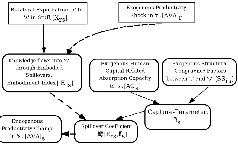
(11) We shall consider an exogenous TFP improvement in the technology for producing Stuff in region r. Specifically, the shock is a Hicks-neutral improvement in the productivity of each primary factor there. Figure 2 shows the way in which technological knowledge embodied in trade flows affects the spillover of productivity from a source to a destination region. Exogenous Productivity. Bi-lateral Exports from 'r' to 's' in Stuff, [X rs ]. Knowledge flows into 's' through Embodied Spillovers; Embodiment Index [ Ers ]. Endogenous Productivity Change in 's', [AVA]s. Shock in 'r', [AVA]r. Exogenous Human Capital Related Absorption Capacity in 's', [AC s ]. Spillover Coefficient,. Exogenous Structural Congruence Factors between 'r' and 's', [SS rs ]. Capture-Parameter, θs. γs [Ers ,θs ]. Figure 2: Flow chart for the transmission mechanism in the model. The improvement in productive efficiency leads to value-added V augmenting technical change in Stuff. Hence, A r in the value-added nest of the production tree [see equation (2.2)] is the appropriate technological change parameter for considering HNTP. In GTAP notation, this is AVA(r). The transmission equation showing how the productivity improvement in r affects productivity in s is as follows: ava(s) = γs(Ers, θs). ava(r). (2.6). where ava(s) and ava(r) are respectively the percentage improvements in the productivity ‘levels’ (HNTP parameters, AVA) in the value-added nest of the production function of regions r and s (the convention in the GTAP system of notation being that the lower case variables represent the percentage changes in the corresponding ‘level’ variables). This transmitted improvement is higher, the higher are the values of ACs and SSrs. More specifically, γ s (E rs , θ s ) = E rs. 1− θs. 7. , 0 ≤ θs ≤ 1. (2.7).

(12) Given the functional form, γ s (E rs , θ s ) ≤ E rs ≤ 1 for 0 < θ s < 1, 0 ≤ E rs ≤ 1 and. ∂γ ′s = − E −rsθ s [1 + ln γ s ] < 0 . ∂θ s. ∂γ ′s < 0 implies that marginal returns of γs to ∂θ s. Ers are a decreasing function of θs . It can also be shown that 1−θ 2 ∂γ s ∂2γ s s = [–γs(Ers).lnErs] > 0 and γ ∂θ s ∂θ 2s = [(lnErs) .Ers ] > 0; i.e., s is a convex function of θs. Thus, the γs function shows increasing marginal returns to θs.10. Substitution of (2.7) into (2.6) shows that, all told, the equation governing the technological spillover is given by ava(s)=Ers. 1-ACs.SSrs. . ava(r). (2.8). Substitution of (2.4) into equation (2.8) yields the fundamental spillover equation for implementation in GTAP as ava(s) = [Xrs/Ys]. 1-ACs.SSrs. . ava(r). (2.8a). Being ‘neutral’ in nature, the exogenous HNTP shock uniformly reduces the input requirements associated with producing a given level of output of Stuff.11. 3. The GTAP Database and Aggregation The aggregation procedure involves working in several steps with the computer files necessary for this task. All these files are documented in detail in the Appendix.. 3.1 Set Aggregation The MODHAR programme available in the Windows version [WINGEM] of GEMPACK (General Equilibrium Modelling Package) was run interactively to create an HAR (Header ARray) file named SET1BY3.HAR from a text file (SET1BY3.TXT) defining the elements of the sets. Table 3.1.1 displays the changes made in the existing SET specifications in the 3×3 database for commodity aggregation.. 10 With the determinants AC and SS of θs both bounded in [0,1] and strictly exogenous, this should not present any computational problem in our GE model. 11 In our current treatment, we do not consider biased technical change of any variety. This rules out closures of the model that correspond to a balanced-growth path (as investigated by Walmsley (1998)). Apart from the exceptional case of a Cobb-Douglas production function, under such closures the only valid sustained technological shock is one which is laboraugmenting (Harrod-Neutral)—see Barro and Sala-I-Martin (1995, Ch 1.) or Powell and Murphy (1997, pp. 97-103);.. 8.

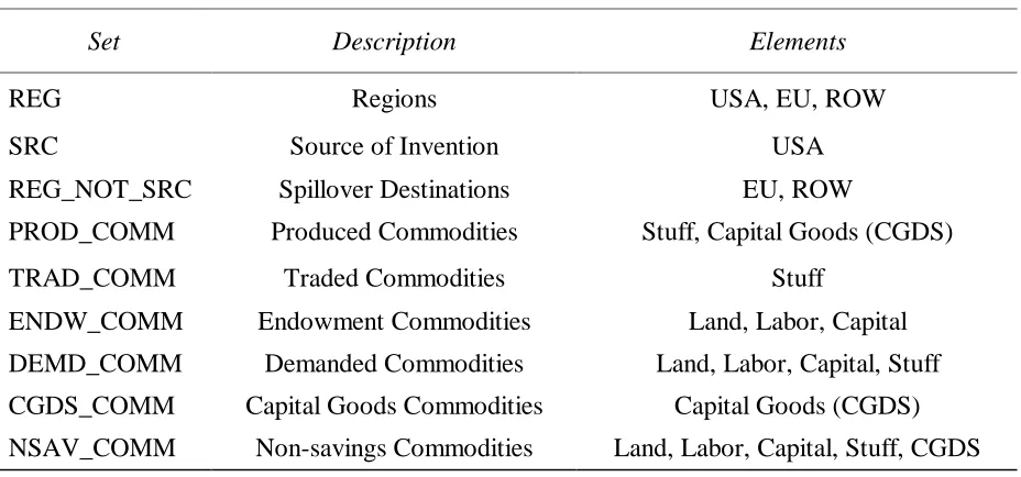
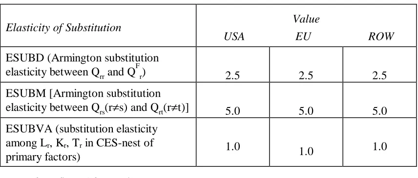
(13) TABLE 3.1.1 List of sets and their elements in 1×3 GTAP Set. Description. Elements. REG. Regions. USA, EU, ROW. SRC. Source of Invention. USA. Spillover Destinations. EU, ROW. PROD_COMM. Produced Commodities. Stuff, Capital Goods (CGDS). TRAD_COMM. Traded Commodities. Stuff. ENDW_COMM. Endowment Commodities. Land, Labor, Capital. DEMD_COMM. Demanded Commodities. Land, Labor, Capital, Stuff. CGDS_COMM. Capital Goods Commodities. Capital Goods (CGDS). NSAV_COMM. Non-savings Commodities. Land, Labor, Capital, Stuff, CGDS. REG_NOT_SRC. 3.2 Database Aggregation We refer to our one-traded-commodity, three-region model as 1×3GTAP. The aggregated database comprising trade, production and input-output data was produced by running Mark Horridge’s programme DAGG on the 3×3GTAP bilateral and input-output data in Version 3 of the data-base as used in GTAP short courses held in August, 1996. It involved a three step procedure as described in details in the Appendix. This database is checked for macro-balance by ensuring that (i) the zero pure profit condition is satisfied; (ii) GDP from the income and expenditure sides match each other.. 3.3 Modification of Parameter Setting The additional parameters introduced in the parameter file are HK(s) and SS(r,s). HK(s) represents ACs as described in Section 2. Their values are set arbitrarily. Assuming that the EU is more similar to the US in both SS and AC than to the ROW, higher values are assigned for these exogenous variables in case of EU as compared to ROW; that is, ACEU > ACROW and SSEU,US > SSROW,US. The Appendix documents them as appended in the TABLO file. The values for the elasticity of substitution parameters (see Table 3.3.1) are assumed to be common across all the regions.. 9.

(14) TABLE 3.3.1 Value of elasticities of substitution parameters*. USA. Value EU. ROW. ESUBD (Armington substitution F elasticity between Qrr and Q r). 2.5. 2.5. 2.5. ESUBM [Armington substitution elasticity between Qrs(r≠s) and Qrt(r≠t)]. 5.0. 5.0. 5.0. 1.0. 1.0. 1.0. Elasticity of Substitution. ESUBVA (substitution elasticity among Lr, Kr, Tr in CES-nest of primary factors) •. Refer to figure 1 for notation.. 4.GTAP Implementation 4.1 Additional Equation The economic model is the one described in Hertel (ed.) (1997) with an additional behavioural equation, two new parameters and two new coefficients, plus some additional national accounting identities coded by Philip D. Adams. Equation (2.8a) in the notation of the GTAP-system of equations is: ava(i,s)= [VXWD(i,r,s)/VOW(i,s)]. (1-AC .SS ). s. rs. . ava(i,r). (2.8b). where i ∈ TRAD_COMM. TRAD_COMM contains traded commodity Stuff only, VXWD(i,r,s) is the value of exports of tradable commodity i from r to s evaluated at world fob prices [i.e., Xrs in equation (2.8a)]; VOW (i,s) is the value of output of tradable commodity i in s evaluated at world fob prices [i.e., Ys in (2.8a)]. The model is encoded in TABLO language for GEMPACK software as reported in the Appendix. In our implementation, we define one region at a time as the source of invention — set named SRC. The countries other than the source belong to the set named REG_NOT_SRC. These two sets are subsets of the set of all regions–REG. Table 4.1.1 gives the encoding of the spillover equation (i.e., equation (2.8b)) in TABLO12 language.. 12. TABLO is an algebraic language for writing economic models and for defining the associated sets, equations, coefficients, and variables for subsequent solution specifically compatible with the GEMPACK software suite (see Harrison and Pearson, 1996).. 10.

(15) TABLE 4.1.1 Additional equation in the TABLO source file for technology spillover Equation MOD_EMB_SPLOVER !This equation gives the Embodied Spillovers via Trade in the recipients! (all, i, TRAD_COMM) (all, r, SRC) (all, s, REG_NOT_SRC) ava(i,s)=[(VXWD(i,r,s)/VOW(i,s))^(1-HK(s)*SS(r,s))]*ava(i,r);. The Appendix documents the changes made in the GTAP96.TAB by defining some additional coefficients, variables and necessary equations.. 4.2 Closure and Shock In the version of GTAP we have used, there is no financial sector. A global ‘bank’ collects regional saving into a hypothetical global saving pool. Saving in each region is conceptually a real ‘saving commodity’ (qsave). After each region receives an allocation of the saving commodity from the global saving pool, it uses the purchasing power so obtained to create new capital. The commodity composition of this new investment (qcgds) is region-specific. All savers face a common price, PSAVE (which is the numeraire in the standard closure of the model), for the savings commodity. The allocation of savings commodity depends on the specification of the closure. Here it is assumed that the aggregate capital stock is exogenous in all regions and that regional and global nett investment move together. While no reallocation of regional shares in global investment is permitted, interindustry capital mobility within a region is allowed. This is known as the medium-run, or partial long-run equilibrium standard closure in the GTAP literature. The parameter RORFLEX(r) determines the sensitivity of regional rates of return to these changes in regional gross investment. Here it is assumed that all regions have RORFLEX(r) =10. In all standard closures of GTAP, the regional labor endowments are exogenous, while in the current closure new investment does not add to the capital stock available in the solution period13. Hence the productive capacities of all regions are unaffected in the period to which the simulation results apply. However, as investment is a component of final demand, it affects economic activity in the solution period via its impact on demand. In 13. We use ‘solution period’ and ‘snapshot’ period interchangeably to mean the period (occurring some time after the shock) for which the simulation is run and solution is obtained. Specifically, we introduce one or more sustained shocks at an initial period and maintain them through until the ‘snapshot’ period is reached. The solution is presented as the percentage deviation in the snapshot period in a variable of interest relative to its value in that period in a base-case or control scenario in which no shocks occur.. 11.

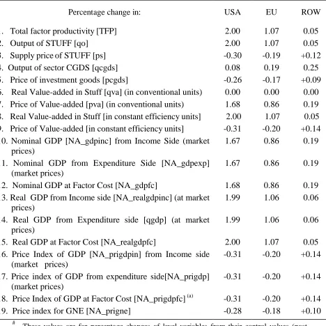
(16) the case of our 1×3 macro aggregation of GTAP, these compositional influences are limited to the sourcing of Stuff from different regions in the assembly of locally-specific capital goods. The notion of TFP improvement in the CGDS sector is not valid as CGDS assembles the Armington substitutable Stuffs for capital formation without using any primary factors of production. Moreover, CGDS is produced and sold solely in the domestic market, and so is non-traded. Whilst the sector’s costs are affected by TFP changes in the three sources of Stuff, CGDS itself plays no role in the technology transfer process. Below we consider an arbitrary 2 per cent TFP shock in the USA in the Stuff sector. In the closure used here, prices, quantities of all nonendowment commodities, and regional incomes are endogenous, while policy variables, other technical change variables, and population [POP(r)] are exogenous to the model.. 5. Analysis of Simulation Results 5.1 Macroeconomic Effects in Each Region Table 5.1.1 summarises the impact of the perturbation on the macro variables. The flow chart in Figure 3 displays a schematic presentation of the simulation results for the macro-variables in the model. With fixed supplies of land, labor and capital and no factor-bias, a 2 per cent TFP-shock in Stuff in the USA leads to an increase in output in that sector and real GDP at factor cost of exactly 2 per cent. After the HNTP shock, we effectively have 2 per cent more of each factor after allowing for the improvement in its quality. Thus, in the snapshot period, one-hundred input-hours of composite real value-added are equivalent to one hundred and two quantity units of composite value-added measured in terms of constant efficiency units applicable in the base-period. Hence, there has been no change in the usage of primary factors of production (as measured in conventional units) between the base case and the shocked solution. This leads to a zero percentage change in value-added (not quality adjusted) by factors of production [row 6, Table 5.1.1]. However, real value-added (measured in constant efficiency units) increases in all three regions. The increase in productive efficiency of the raw primary composite input (measured in conventional units) leads to an increase in its marginal productivity (MP) — i.e., 2.00, 1.07, and 0.05 per cent for USA, EU and ROW respectively 14. Since factors are paid according to their marginal. 14. The percentage changes in marginal (physical) productivities can be verified from computed GTAP variables as follows. In the levels, the value of the MPs of factors should equal their prices: Pstuff * MPf = Pf ( where f∈{L, K, T}). 12.

(17) TABLE 5.1.1. Simulated regional effects of technological change in the USA on selected macroeconomic variables#. Percentage change in:. USA. EU. ROW. 1. Total factor productivity [TFP] 2. Output of STUFF [qo] 3. Supply price of STUFF [ps] 4. Output of sector CGDS [qcgds] 5. Price of investment goods [pcgds] 6. Real Value-added in Stuff [qva] (in conventional units) 7. Price of Value-added [pva] (in conventional units) 8. Real Value-added in Stuff [in constant efficiency units] 9. Price of Value-added [in constant efficiency units] 10. Nominal GDP [NA_gdpinc] from Income Side (market prices) 11. Nominal GDP from Expenditure Side [NA_gdpexp] (market prices) 12. Nominal GDP at Factor Cost [NA_gdpfc] 13. Real GDP from Income side [NA_realgdpinc] (at market prices) 14. Real GDP from Expenditure side [qgdp] (at market prices) 15. Real GDP at Factor Cost [NA_realgdpfc] 16. Price Index of GDP [NA_prigdpin] from Income side (market prices) 17. Price index of GDP from expenditure side[NA_prigdp] (market prices) 18. Price Index of GDP at Factor Cost [NA_prigdpfc] (a) 19. Price index for GNE [NA_prigne]. 2.00 2.00 -0.30 0.08 -0.26 0.00 1.68 2.00 -0.31 1.67. 1.07 1.07 -0.19 0.19 -0.17 0.00 0.86 1.07 -0.20 0.86. 0.05 0.05 +0.12 0.25 +0.09 0.00 0.19 0.05 +0.14 0.19. 1.67. 0.86. 0.19. 1.68 1.99. 0.86 1.06. 0.19 0.06. 1.99. 1.06. 0.06. 2.00 -0.31. 1.07 -0.20. 0.05 +0.14. -0.31. -0.20. +0.14. -0.31 -0.28. -0.20 -0.18. +0.14 +0.10. #. These values are for percentage changes of level variables from their control values (postshock). Figures are rounded to 2 or 3 decimal places. The shock is a 2 per cent increase in TFP. (a) Figures for row 18 are obtained by modifying the existing equation for it in GTAP National Accounts module à la Adams (1996) and incorporating into it the ‘Tec_Chg’ variable as documented in the Appendix. These are the same as figures in row 9 after this adjustment has been made.. We have computed GTAP results for the percentage changes in Pstuff and in each Pf—pstuff, pL, pK, and pT (say)—in each region. Then, for example, we can use the above relationship to compute the percentage change in the marginal physical product of labour by: (initial) (initial) * (1+pf/100)] / [Pstuff * (1+pstuff/100)]}-1)*100 per cent change in MPL= ({[Pf = 100* [{(pf/100)-(pstuff/100)}/(1+pstuff/100)] Note that this accurate calculation is not replicated by simply subtracting ‘pstuff’ from ‘pl ’.. 13.

(18) A. TECHNOLOGY TRANSMISSION BLOCK Real Value-added (Quality Adjusted) increases in all regions. 2% TFP Shock in source USA. Technology Transmission via trade and AC and SS to Destinations EU, ROW. Real regional income increases more than real GDP at market prices in all regions. Increase in real and nominal privexp, govexp, qsave. Increase in Marginal Productivity of primary factors equal to the TFP shock. Increase in Returns to primary factors (in conventional units) and change in price of quality-adjusted inputs. Supply price of Stuff falls in USA and EU and rises in ROW. Terms-of-trade falls in USA and EU and rises in ROW. GDP deflator falls in USA and EU,rises in ROW. Price index of GDP at factor cost falls in USA and EU and rises in ROW. CPI, price index of public purchase and prigne fall in USA and EU, and increase in ROW. qsave in ROW is less than that in USA and EU. B. REGIONAL INVESTMENT ALLOCATION BLOCK. Medium -run closure i.e., fixed regional composition of global investible funds in base-period proportion. Regional and Global net investment move together. Increase in regional real gross investment demand (qcgds) in all regions. qcgds in ROW is higher than that in USA and EU Trade balance improves in USA and EU and deteriorates in ROW For USA and EU, qsave is higher than qcgds; for ROW, qsave is less than qcgds. Rise in Imports for CGDS in ROW. Figure 3: Flow chart showing the principal pathways behind the results. 14.

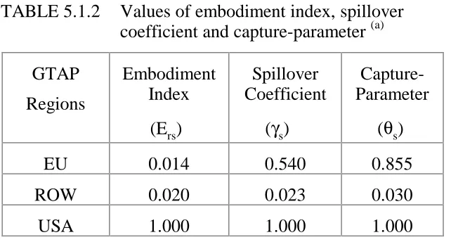
(19) products, these increases in MP lead to increases in the price of value-added and their constituents in all three regions. Being neutral in nature, this TFP improvement causes equal percentage increases in the real rewards of all primary factors within any given region. We observe that there has not been full transmission of technical change from the source to the destinations — EU and ROW. Table 5.1.2 suggests that the value of the spillover coefficient depends more strongly on θs than on Ers alone. Thus, whilst trade is the prime vehicle for transmission of knowledge flows, ACs and SSrs (and hence, θs ) are critical for effective transmission of technology from r to s. This is supported by the fact that even when Ers has lower values, the magnification of them by θs can lead to a high rate of capture of the technological improvement. Thus, EU with higher values of both ACs and SSrs, does better than ROW at capturing the TFP improvement occurring in the USA despite ROW having a higher value of Ers. Consequently, in Table 5.1.1 we see a greater improvement in technology in EU (1.07) as compared to that in ROW (0.05). TABLE 5.1.2. GTAP Regions. Values of embodiment index, spillover coefficient and capture-parameter (a) Embodiment Index. Spillover Coefficient. CaptureParameter. (Ers). (γs). EU. 0.014. 0.540. 0.855. ROW. 0.020. 0.023. 0.030. USA. 1.000. 1.000. 1.000. (θs). (a) Values shown relate to the pre-shock situation.. Stuff being the only sector whose production involves value-added, its share in total value-added is unity in all three regions. As the TFP improvements cause real value-added by factors of production (quality adjusted) to increase by the same percentages, the percentage change in real GDP at factor cost in each region is equal to the respective TFP shock (see rows 1 and 8, Table 5.1.1). Also, the price indexes for value-added in Stuff (row 9 of Table 5.1.1) and for GDP at factor cost (row 18) are identical. Changes in real nett indirect taxes (which are of fairly small magnitude) account for the wedges between real GDP at market prices and real GDP at factor cost. Now, the recorded nominal GDP at factor cost [NA_gdpfc] (row 12, Table 5.1.1) is calculated on the basis of price and quantity indexes of valueadded measured in conventional units [pva]. These are taken as given from the GTAP results. As the real value-added measured in constant efficiency units (i.e., ‘quality-adjusted’) increases in all regions by the same percentage. 15.

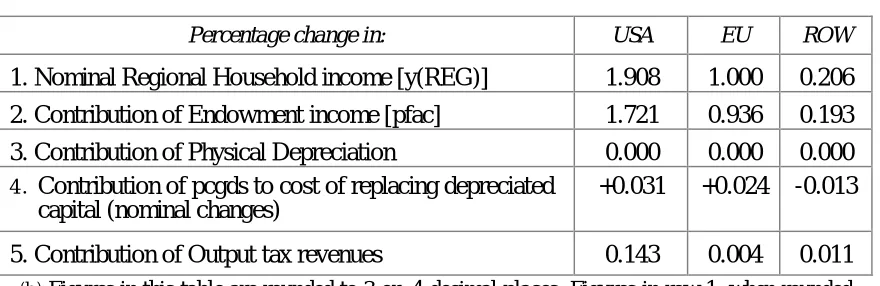
(20) as the TFP improvement, the effective price of value-added has to adjust accordingly so that the nominal value-added measured in constant efficiency units matches the GTAP results. The increases in real value-added (measured in constant efficiency units) of about 2 and 1 per cent respectively in USA and EU lead to falls in the corresponding price indices of about 0.3 and 0.2 per cent (rows 8 and 9, Table 5.1.1). In case of ROW, the small rise in real value-added (with least TFP improvement) is not enough to depress the corresponding price given the attendant general equilibrium effects (to be discussed below) — in fact, it rises there by 0.14 per cent.. 5.2 Inter-regional Competition Effects Table 5.2.1 shows that, region by region, there have been increases in nominal regional household income [y(r)] and its uses ( rows 1, 7, 5 and 4). We first explain post-shock differential impacts on nominal income [y(r)] which is the sum of primary factor payments and receipts from various transactions taxes nett of depreciation. Table 5.2.2 breaks up the componentwise effects on y(r). Earlier discussion shows that the HNTP shock increases ‘pva’ and its components (row 7, Table 5.1.1). The increase in y(r) has primarily been caused by the uniform increases in primary factor payments in all regions (row 2, Table 5.2.2). With fixed regional supplies of capital stocks at the beginning of the solution period, ex post there have been no percentage changes in it and hence none in physical depreciation (row 3). Changes in the price of capital goods (pcgds) cause a revaluation of existing capital stock; however, capital gains/losses do not enter into our definition of regional income. But changes in pcgds affect the cost of capital consumption, which enters our income definition as a debit. As pcgds falls in the USA and EU (row 5, Table 5.1.1), the replacement cost of existing capital goods falls in these regions (row 4, Table 5.2.2), contributing small rises to nett incomes. In case of ROW, the increase in pcgds causes the nominal cost of replacing depreciated capital to go up and this, in turn, dampens the effect of the small increase in endowment income. With exogenously fixed tax rates, the changes in prices reflect only the effects of the TFP shock per se. Given output tax rates, an increase in output causes a rise in tax revenues on commodities (row 5, Table 5.2.2).. 16.

(21) TABLE 5.2.1 Simulated regional effects on sources of final demand Percentage change in:. Θ. USA. EU. ROW. 1. Regional household income [y (REG)] (Nominal). 1.91. 1.00. 0.21. 2. Price index of GDP from expenditure and income sides(market prices). -0.31. -0.20. +0.14. 3. Regional household income [u (REG) ] (Real). 2.19. 1.17. 0.12. 4.Regional nett savings demand [qsave] (Real and nominal) Φ. 1.91. 1.00. 0.21. 5. (Real) Public consumption [ug (REG)]. 2.20. 1.19. 0.09. 6. Nominal Public consumption [yg(r)]. 1.91. 1.00. 0.21. 7. Nominal Private household expenditure [yp(REG)]. 1.91. 1.00. 0.21. 8. (Real) Private household consumption [up (REG)]. 2.19. 1.18. 0.10. 9. Gross National Expenditure (NA_realgne ] (Real). 1.92. 0.99. 0.14. 10. Price index for GNE [NA_prigne]. -0.28. -0.18. +0.10. 11. McDougall Terms-of-trade (McDougall_TOT). -0.35. -0.21. +0.17. 12. Aggregate export price index of Stuff [pxw]. -0.30. -0.19. +0.12. 13. Aggregate import price index of Stuff [piw]. +0.05. +0.02. -0.05. 14. Real value of exports [qxw]. 1.71. 1.19. 0.05. 15. Real value of imports [qiw]. 1.01. 0.50. 0.46. 16. Change in trade balance [DTBAL] ψ. +1508.26 +3233.6. -4741.86. 17. Consumer price index [ppriv]. -0.277. -0.179. +0.104. 18. Government aggregate purchase price index [pgov]. -0.285. -0.189. +0.110. 19. Real GDP from Expenditure and Income sides (market prices). 1.99. 1.06. 0.06. 20. Real Gross regional investment [qcgds]. 0.08. 0.19. 0.25. Θ Figures in this table are rounded to 2 or, 3 decimal places. Φ This is the same in ‘nominal’ terms as there has been no per cent-change in its price PSAVE. ψ Since the trade balance can pass through zero, percentage changes are avoided in the case of this variable. The change reported here is an ordinary change (million US $) changes of level values.. 17.

(22) TABLE 5.2.2 Simulated effects on nominal regional income Percentage change in:. (b). USA. EU. ROW. 1. Nominal Regional Household income [y(REG)]. 1.908. 1.000. 0.206. 2. Contribution of Endowment income [pfac]. 1.721. 0.936. 0.193. 3. Contribution of Physical Depreciation 4. Contribution of pcgds to cost of replacing depreciated capital (nominal changes). 0.000 +0.031. 0.000 +0.024. 0.000 -0.013. 5. Contribution of Output tax revenues. 0.143. 0.004. 0.011. (b). Figures in this table are rounded to 3 or, 4 decimal places. Figures in row 1, when rounded to 2 decimal places, yield the same figures as in row 1 of Table 5.2.1. We do not report here the figures for all component-wise effects from tax receipts. Figures of very small magnitude ( < 0.00003) are excluded.. We now turn to the discussion of impacts on sources of various income uses. 5.2.a Region-wide impact on sources of final demands. In GTAP, each region’s demands for private expenditure [PRIVEXP(r)], public expenditure [GOVEXP(r)] and saving [SAVE(r)] are determined by maximisation of a per capita Cobb-Douglas utility function subject to the constraint that these three items totally exhaust the regional income [INCOME(r)]. Under this specification, their fixed shares of income result in the equality of percentage increases in nominal demand for the income uses with the percentage increases in total nominal income. In the present closure with PSAVE as the numeraire, the percentage increase qsave is the same as that in nominal income and changes in real and nominal saving, qsave, are the same. Given the equality of percentage changes in the nominal variables15 PRIVEXP and GOVEXP in each region, we observe that the corresponding real variables in each region move together but not strictly in proportion to each other (see rows 5 and 7, Table 5.2.1). The changes in real consumption expenditures are attributed to the differential impacts of movements in pgov (the aggregate government purchase price index) and ppriv (the consumer price index or, CPI) — the divergence being caused by the diverse purchase patterns of the private and public ‘households’16. Back-of-the-envelope calculation shows that changes up(r) and ug(r) are almost exactly the differences between percentage changes in nominal PRIVEXP and. 15. 16. In terms of the TABLO file, strictly speaking, PRIVEXP and GOVEXP are coefficients which are equal to the levels values of the variables ‘yp’ and ‘yg’. The latter one is added in the original TABLO file for computational conveniences. According to base-period data, the share of domestic Stuff in government consumption is 96 per cent for USA, 99 per cent for EU and 97 per cent for ROW. This is higher than that in the private sector’s consumption — 95 per cent for USA, 96 per cent for EU, and 93 per cent for ROW. As well, the regional composition of imported Stuff differs between the two categories of consumption.. 18.

(23) GOVEXP (rows 6 and 7, Table 5.2.1) and ppriv and pgov respectively (rows 17 and 18, Table 5.2.1). The private household price index (pp) and government household price index (pg) are both share weighted averages of percentage changes in a composite import price index and in a domestic price index for domestic Stuff at purchaser’s prices. For each category of consumption, domestically-sourced Stuff represents a larger share (on an average 96 per cent for GOVEXP and 93 per cent for PRIVEXP) than composite imports in all three regions. With domestically sourced Stuff dominating the CPI in every region, the falls in the price of Stuff in USA and EU by 0.30 and 0.19 per cent respectively translate into declines in the CPI in these two regions of 0.28 and 0.18 per cent respectively. Similar considerations explain the slightly larger falls of the pgov in these two countries — compare rows 17 and 18 in Table 5.2.1. For ROW, on the other hand, the increase in the price of domestic Stuff by 0.12 per cent leads to a 0.10 per cent increase in the CPI whereas pgov registers a slightly larger percentage rise (0.11) there. Now, the percentage increases in real private and public consumption demand for composite Stuff are larger than the corresponding increases in domestic supply in every region (rows 5 and 8, Table 5.2.1 and row 2, Table 5.1.1). In spite of the small percentage increments in the market price of composite imports in USA (0.05) and EU (0.02), this leads to increases in private household import demands of 1.35 and 0.7 per cent in USA and EU respectively17. The much larger fall in the price of domestically sourced Stuff — 0.3 per cent in USA and 0.19 per cent in EU — causes the relative price of domestic- vis-a-vis foreign-sourced Stuff to fall by 0.35 and 0.21 per cent in USA and EU respectively. Given the expansionary effect on demand (qp) for composite Stuff due to the general increase in consumption demand, this leads to substitution in favour of domestic Stuff in USA and EU and reinforces the expansion effect. This is reflected in increases of 2.2 and 1.2 per cent in private consumption demand for domestic Stuff in USA and EU respectively. As opposed to this, in the case of ROW, a decline in the price of composite imports by 0.05 per cent and a rise of 0.12 per cent in the price of domestic Stuff causes the relative price of domestic Stuff to increase by 0.17 per cent. This leads to substitution in favour of imported Stuff with a relatively larger percentage increase (0.5) in demand for foreign composite Stuff as compared to that in domestic Stuff (0.07). Since Armington elasticities are the same across uses and regions, similar considerations apply in the case of public consumption. 17. The share of imports by public and private sectors together in aggregate imports of tradable Stuff are 38 per cent for USA, 21 per cent for EU and 22 per cent for ROW. The rest of aggregate imports of Stuff are used as intermediate inputs by firms producing Stuff and CGDS. Firms’ demand for composite Stuff as intermediate inputs also changes and this, in turn, affects changes in aggregate region-wide imports of Stuff. We do not discuss this at least for the time-being.. 19.

(24) The aggregate utility index [u(r)] proxies regional real income18. In the model, percentage changes in the sub-utility indexes for the public [ug(r)] and private [up(r)] household consumption are equal to the percentage changes in real quantities purchased by the representative government and private households respectively. The Cobb-Douglas utility function is self-dual19 as it generates an unit cost function of the same functional form as the primal. Following this property, the income deflator [incdeflator(r)] for y(r) is defined as the sum over the products obtained by multiplying the CobbDouglas price indexes for each income use viz., ppriv(r), pgov(r) and psave with their corresponding region-wise shares in total income20. Table 5.2.3 reports the values of the shares — i.e., PRIVEXP/INCOME, GOVEXP/ INCOME, SAVE/INCOME and the incdefaltor(r). Row 4 in Table 5.2.3 shows that incdeflator(r) preserves the same ranking, sign and order of magnitude as the ppriv and pgov (rows 17 and 18, Table 5.2.1). Subtracting row 4 of Table 5.2.3 from row 1 of Table 5.2.1, we reproduce, almost exactly, the results on real income (row 3, Table 5.2.1). TABLE 5.2.3 Budget shares of each income use category and incdeflator(c) Values of:. USA. EU. ROW. 1. PRIVEXP/INCOME. 0.7711. 0.7017. 0.6926. 2. GOVEXP/INCOME. 0.2108. 0.2158. 0.1515. 3. QSAVE/INCOME. 0.0181. 0.0825. 0.1559. -0.27. -0.17. +0.09. 4. incdeflator (c). 18. 19. 20. The shares are calculated from base-period data and hence these are base-case values; under the Cobb-Douglas specification, these are unchanging parameters.. In percentage change form, the first-order condition for this optimisation exercise yields: u (r) = [PRIVEXP (r)/INCOME (r)] ∗ up (r) + [GOVEXP (r)/INCOME (r)] ∗ ug (r) + [SAVE (r)/INCOME (r)] ∗ qsave (r) Thus, percentage changes in real income are calculated by summing over the percentage changes in the sub-utility indexes multiplied by their corresponding shares in aggregate income. The duality between production and cost function is formally analogous to the duality between utility and expenditure function—this implies that minimization of total outlay on public and private consumption and saving subject to the specified level of utility will give the same demand equations for these income uses. For a discussion on ‘self-duality’ between CobbDouglas production and cost function, see Varian (1984) Microeconomic Analysis, 2nd edition, pp. 62-64, 69-73. The mathematical expression for incdeflator (r) is: incdeflator (r) = [PRIVEXP (r)/INCOME (r)] ∗ ppriv (r) + [ GOVEXP (r)/INCOME (r)] ∗ pgov (r) + [SAVE (r)/INCOME (r)] ∗ psave. With PSAVE being the numeraire in the model, psave = 0 so that the last term in the equation vanishes to yield the price index for income in general.. 20.

(25) Now, the GDP deflator (pgdp) is weighted sum of percentage changes in the index of the price of the domestic absorption (NA_prigne), in the export price index (pxw), in the price index for exports to the international transportation sector (pm) and in the aggregate import price index (pim) — the weights being the shares in GDP of gross national expenditure (GNE), of exports (VXWD), of sales to the global transport sector (VST), and of imports (VIWS)21. pgdp includes the change in the price of exportable Stuff (pxw) with a positive weight that includes exports rather than just domestic consumption — as in the case of NA_prigne. Also, pgdp includes pim with a negative weight. Hence, the percentage increase pim and the percentage fall pxw lead to a more negative change in pgdp than NA_prigne. Now, the consumption deflators include the price of imports with positive weight. These consumption deflators are included in NA_prigne and thus, it includes the import price index with a positive weight. From Table 5.2.4, it is evident that the difference between pgdp and NA_prigne clearly relates to the percentage deviation of the terms-of-trade (TOT ) from the control scenario22. The fall in TOT in USA and EU does not cause CPI, pgov and hence, NA_prigne to fall as much as pgdp — see rows 1 and 5 in Table 5.2.4. This implies that a decline in TOT implies a rise in the consumption deflators (which include price of imports) relative to pgdp (which includes price of exports) in these regions. Similar considerations explain relatively larger percentage changes in pgdp relative to NA_prigne and the consumption deflators in case of ROW. In our simulation, an increase in nominal income [y(r)] leads to equiproportionate increases yp(r) and yg(r) for any given region (as discussed in subsection 5.2.a). For USA and EU, CPI and ‘pgov’ do not fall as much as the GDP deflators and this results in comparatively higher 21. 22. The GDP deflator, pgdp, can be broken down into the following components as below: pgdp=NA_prigne*(GNE/GDP)+pxw*(VXWD/GDP)+pm*(VST/GDP)-pim*(VIWS/GDP) It is to be noted that ‘pm’ and ‘pxw’ are the same. Nominal domestic absorption, GNE(r) is expressed as: GNE(r)= PRIVEXP(r)+GOVEXP(r)+REGINV(r). Thus, the GNE deflator is: NA_prigne(r)=ppriv(r)∗[PRIVEXP(r)/GNE(r)]+pgov(r)∗[GOVEXP(r)/GNE(r)]+ pcgds(r)∗ [REGINV(r)/GNE(r)]. After some algebraic manipulation, we can re-write the expression in Footnote 21 as: pgdp−NA_prigne=[pxw*{(VXWD+VST)/GNE}]−[pim*(VIWS/GNE)]−pgdp*(TradeBalance /GNE)] In the case of balanced trade, VXWD+VST=VXW=VIWS, this equation becomes: pgdp−NA_prigne = (VIWS/GNE) (pxw − pim). Also, in case of balanced trade, GNE (r)=GDP (r). Thus, multiplying both sides of the above expression by [GNE/GDP], we rewrite it as: pgdp−NA_prigne = [pxw−pim]∗[VIWS/GDP] = [VXW/GDP] ∗ [pxw−pim] The variable (pxw − pim), the percentage change in the ratio of export prices to import prices, is a conventional measure of the change in the terms-of-trade. Although the GTAP standard TOT definition also includes the price of the non-traded regional investment goods, QO(CGDS, r), here we use the more conventional definition introduced above.. 21.

(26) TABLE 5.2.4 Component-wise effects on pgdp (f) Share weighted values of:. USA. EU. ROW. 1. GNE deflator [=NA_prigne* GNE/GDP]. -0.278. -0.180. +0.101. 2. Price of exports [=pxw × Exports/GDP]. -0.029. -0.020. +0.025. 3. Price of imports [= pim × Imports/GDP]. +0.005. +0.002. -0.010. 4. Price of exports for global transportation sector[=pm×VST /GDP]. -0.001. -0.003. +0.001. 5. Percentage changes in GDP price deflator [pgdp = (1)+ (2)+ (4)-(3)]. -0.313. -0.205. +0.137. (f) Calculated from base-period data. Figures in row 5 match the figures in row 2 in Table 5.2.1 when we do ‘rounding’ to 2 decimal places.. percentage increases in real consumption than in real GDP. In the case of ROW, relatively smaller percentage increases in the consumption deflators than in pgdp cause the percentage change in real consumption to be higher than in real GDP (row 5, 8 and 19 in Table 5.2.1). In the base-case, for both USA and EU, nominal GNE exceeds GDP (and hence, each has an initial trade deficit) whereas in ROW, GDP outweighs GNE (and hence, ROW has initial trade surplus). However, despite moving in the same direction in every region, real GNE [NA_realgne(r) ] diverges from real GDP [qgdp(r) ] — compare rows 9 and 19 in 5.2.123. GNE includes gross investment expenditure — the value of output of the capital goods sector [REGINV(r)]. We now turn to the explanation of why the investment results look the way they do.. 23. We can write in nominal terms, GDP (r) = GNE (r) + TBAL (r) where TBAL (r) is the regional trade balance. Thus, in percentage change form we get gdp (r) = gne (r) ∗ [GNE (r)/ GDP (r)] + DTBAL (r)/GDP (r) where DTBAL is the ordinary change in TBAL. Using the expression for [pgdp − NA_ prigne] when TBAL ≠ 0 [as in Footnote 23] and the expression for gdp (r) as derived above, algebraic manipulation yields, for any region, the difference between qgdp and NA_realgne as: qgdp − NA_realgne = DTBAL/GDP − [TBAL/GDP ] ∗ NA_realgne − [ pxw ∗ (VXW/GDP ) − pim ∗ (VIWS/GDP )] When TBAL = 0, i.e., there is balanced trade so that VXW = VIWS, DTBAL = 0, the above difference can be written as: qgdp − NA_realgne = − [VIWS/GDP] ∗ (pxw − pim). Thus, the differential between qgdp and realgne is ascribed to changes in TOT and relevant trade share/s.. 22.

(27) 5.2.b Regional Effect of investment allocation mechanism§ The increase in pva and each of its components by the same percentage leads to an increase in the rental or supply price of capital as an input into production in every region by the same magnitude as ‘pva’ — compare row 3 in Table 5.2.5 with row 7 in Table 5.1.1. TABLE 5.2.5. Simulated effects on rate of returns and base-period values of some coefficients(f). Values of:. USA. EU. ROW. 1. GRNETRATIO [r]. 1.516. 1.607. 1.447. 2. INVKERATIO [r]. 0.048. 0.064. 0.079. 3. Per cent changes in Rental price of capital [ps(Capital,r)]. 1.68. 0.86. 0.19. 4.Per cent changes in Price of CGDS [ps(CGDS,r) = pcgds (r)]. -0.26. -0.17. +0.09. 5. Per cent changes in Current nett rate of return [rorc(r)]. 2.94. 1.66. 0.14. 6. Per cent changes in Expected nett rate of return [rore(r)]. 2.90. 1.54. -0.06. 7. Per cent changes in End of period capital stock [ke(r)]. 0.004. 0.012. 0.02. (f) The figures in this Table are rounded to 2 or, 3 decimal places. Values for the coefficients are. reported from base period data.. With PSAVE being the numeraire in the model (as in the base-case), the price of the global saving good is unaltered in any simulation. As explained in subsection 5.2.a, the increases in y(r) lead to equal percentage increases in the corresponding regional demands for nett savings, qsave (nominal and real) which are aggregated into a global nett saving pool so that the global supply of saving — used to finance global expenditure on nett investment — increases following the shock. The percentage increase in the global supply of capital goods composite [globalcgds] is a weighted average of qsave (row 4, Table 5.2.1)24. As all other markets are in equilibrium (which is checked by inspecting the updated post-simulation data-base), the market for the ‘saving’ commodity must clear à la Walràs’ Law. We checked that the §. 24. Space limitations prevent us from reporting all the calculations in this section. As has been mentioned elsewhere, since CGDS is non-traded and investment is not available online for production in the solution period, the investment allocation mechanism does not enrich the story associated with the technology transmission via trade. This consideration made us parsimonious while drafting this section. However, interested readers can contact the author for an unabridged version of this particular section named “Elaboration of investment allocation mechanism”. The formula used for this calculation is: globalcgds = ∑r [SAVE(r)/GLOBINV] ∗ qsave (r). The values for these shares in the base case are 0.048, 0.242 and 0.71 for USA, EU and ROW respectively.. 23.

(28) endogenous walraslack variable is zero to ensure market-clearing in the omitted market and post-shock equilibrium in the global economy. Since the portfolio of regional nett saving commodities provides a composite investible fund, the increase globalcgds [≡ walras_sup] in the omitted market translates into a matching change in global nett saving demand [walras_dem] as well in that market. In this closure, as the world pool of the real CGDS composite is distributed across regions in the same fixed proportion25 of NETINV(r) to GLOBINV as in the base-case, because of its higher base-period proportion, ROW gets a larger allocation (67 per cent) from the global nett saving pool than USA (7 per cent), while EU receives the remainder (26 per cent). Given the fixity of the regional composition of global nett investment, the region-specific ratios of NETINV(r) to the GLOBINV pool are (in the solution period) unchanged from the base case, so the percentage changes in regional real nett investment demand are equal to globalcgds i.e., 0.48 per cent. Regional demand for real gross domestic capital formation [qcgds(r)] is determined by multiplying a region-specific ratio of conversion from nett to gross investment26. Thus, the allocation mechanism causes real gross investment demand in ROW to increase by a higher percentage than in USA and EU, leading to a surge in GNE relative to GDP in ROW. In the control scenario, USA and EU had trade account deficits and ROW had a trade surplus. According to the TFP shock-induced mechanism, USA and EU are able to reduce their trade and saving deficits, whereas ROW sees a fall in its surpluses (compare Tables 5.2.6a with 5.2.6b). Whilst ROW receives a higher allocation of globalcgds than USA and EU, the percentage increase in saving in ROW, (qsave) is less than that in USA and EU (see row 4, Table 5.2.1). This follows from the fixed budget-share of regional saving in regional income under the Cobb-Douglas specification. However, a fall in the level of gross investment in USA as opposed to a relatively large rise in the level of gross saving has caused a reduction in the saving gap there. In the case of EU, a modest rise in gross saving coupled with a very weak rise in gross investment has managed to reduce the saving gap in this region also (compare rows 3, Tables 5.2.6a and 5.2.6b). As there has. 25. 26. Here the proportion refers to the base-case values of a region-specific ratio— NETINV(r)/GLOBINV, where GLOBINV = ∑ r NETINV (r) and NETINV (r) is regional nett investment. These ratios differ from the corresponding regional shares of the global capital stock in the data-base. There is nothing to ensure that the region-wise beginning of period capital stock to global capital stock ratio is kept constant during a simulation. Consequently, the ratio applied here must be interpreted strictly in terms of region-wise fixed nett investment flows. The values for the ‘proportion’ of NETINV(r) to REGINV(r) calculated as per the base-case data are respectively 0.176, 0.389 and 0.514 for USA, EU and ROW. The increase qcgds(r) is this ratio times the percentage deviation (0.48) of regional nett investment demand from the base-case.. 24.

(29) TABLE 5.2.6a Base-case values of Gross Saving and Gross Investment(~) EU. ROW. SUM over rows. 737401.9. 1304481.97. 2679526.5. _. 2. Gross Investment [REGINV(r)]. 779940. 1343140. 2598330. _. 3. Saving Gap [ (1) - (2) ]. -42538. -38658. +81196. 0.00. 4. Trade balance (in million U.S. $). -42538. -38656. +81200. 6.00. Base-case values of: 1. Gross Saving. USA. (~) Calculated from base-period data by adding the depreciation figures to net saving and investment figures.. TABLE 5.2.6b Post-shock values of Gross Saving and Gross Investment(!). Simulated values of:. USA. EU. ROW. SUM over rows. 1. Gross Saving. 737557.33. 1307913.4. 2683641.3. _. 2. Gross Investment. 778587.87. 1343336.94. 2607190. _. -41030.5. -35423.5. +76451.3. -2.70. -41029. -35423. +76450. -2.00. 3. Saving Gap [ (1) - (2) ] 4.. Trade balance (in million U.S. $). (!) Based on the post-solution data using the same procedure as in case of Table 5.2.8a.. been a higher percentage increase in the value of exports than in the value of imports in both USA and EU, the trade deficits in these two regions are reduced. These improvements in trade balances are equal to the differences between row 4 of Table 5.2.6b and the same row in Table 5.2.6a; they account for the ‘reduced’ saving deficits in USA and EU so that the declines in the trade deficits almost exactly match the reductions in the saving gaps. As is evident from Tables 5.2.6a and 5.2.6b, ROW initially had a ‘saving surplus’ to lend investible funds to USA and EU. After the shock, ROW is still a nett external creditor to USA and EU, although not as strongly so as previously. We see that ROW’s surplus has declined by US $ 4744.7 million. However, the TFP shock causes the value of imports of Stuff in ROW to rise by a larger proportion (0.403 per cent) than that of its exports (0.16 per cent). This is associated with a fall of US $ 4750 million in the trade surplus in ROW (compare rows 4, Tables 5.2.6a and 5.2.6b). Not having generated adequate domestic saving for meeting its relatively large gross investment demand, ROW must finance the gap by capital inflow, which shows up here as a fall in its trade surplus. This is matched by the sum of the improvements in the trade balances of USA and. 25.

(30) EU (the sources of the capital inflows)27. In the solution period, the sum over regions of the differences between gross regional saving and investment [regional savings gap] equals zero (excepting the discrepancy due to the rounding errors) as does the sum of the regional trade balances28. In this closure, regional capital stocks in use are kept at their control equilibrium values [fixed capital stocks (KB(r))].With full capacity utilization, the percentage changes in the flow of capital services, ksvces(r), from these stocks, also remain unchanged.29 As the percentage change in KE(r)30 depends on the change in real gross investment flows in a region and on the base-period value of INVKERATIO(r) — the ratio of gross regional investment [REGINV(r)] to [ KE(r) ] — higher values of INVKERATIO(r) and qcgds(r) in ROW are reflected in relatively larger percentage changes in its end-of-period capital stock as compared to that in EU and USA (row 7, Table 5.2.5). Assumption of identical sensitivity of the prospective rate of return (for the period following the solution period) to the prospective proportional expansion in the regional capital stock across all regions implies that a relatively larger percentage increase in KE(r) and a smaller value of current rates of return rorc(r)31 in ROW cause rore(r) to fall there.32 On the other hand, a relatively larger rorc(r) and very small percentage increases in KE (r) in USA and EU causes rore(r) to increase in the period following the solution period in these two regions (row 6, Table 5.2.5).33. 27 28. 29 30. 31. 32. 33. In GTAP, there is no option for meeting the current account deficit by ‘equity investment flow’ mechanism. The only way to meet the ‘gap’ is by incurring new debts from overseas. Since for each region, Gross Save (r)– REGINV (r)= VXW (r)–VIW (r), for the global economy as a whole to be in equilibrium, ∑r [Gross Save (r)– REGINV (r)]= ∑r [VXW (r)– VIW (r)]= 0. Here, fixing aggregate capital stock exogenously means flow of services from that stock in the solution period, ksvces(r)=0. In levels form, the stock-flow relation for KE(r) and KB(r) is: KE(r)= KB(r)*[1-DEP(r)] + REGINV(r). Corresponding percentage change form is given by: ke(r)= INVKERATIO(r)* qcgds (r) + kb(r) * [1- INVKERATIO (r)]. When kb(r)=0, ke(r) is endogenously determined by changes in gross real regional investment—qcgds(r). In level form, rorc (r) is expressed as: RORC(r)= [RENTAL(r)/PCGDS(r)]-VDEP(r). The corresponding percentage change form is: rorc(r)= GRNETRATIO (r) * [rental (r)-pcgds(r)] where GRNETRATIO (r) is the ratio of the gross to the nett rate of return in region r. -RORFLEX(r) In levels form, prospective rate of return is: RORE(r)= RORC(r)*[KE(r)/KB(r)] where RORFLEX(r) = 10 is a parameter—for explanation, see Section 4.2 above. The corresponding percentage change form is: rore(r)= rorc(r)−RORFLEX(r)*[ke(r)−kb(r)] = rorc(r)−RORFLEX(r)*[INVKERATIO(r)*qcgds(r)− kb(r)*INVKERATIO(r)]. With kb(r)=0 and given INVKERATIO(r), rore(r) depends on rorc(r) and qcgds(r). Note that these changes are percentage, not percentage-point, changes in expected rates of return.. 26.

(31) 5.2.c Regional composition of international trade Due to the Armington specification of commodity substitution, even in a world with one generic traded-commodity in every region, the relative price divergences (between the three varieties of Stuff) across regions (after the TFP shock) induce changes in regional TOT and open up the scope for interregional competition via trade. Consequently, these lead to changes in the regional composition of exports and imports depending, inter alia, on the movements in TOT. Looking at the global economy as a whole, we observe that after the shock there has been an increase in the quantity index of global merchandise exports and imports of Armington substitutable Stuffs by 0.57 per cent34. However, ROW experiences a small percentage rise in the price of domestically produced Stuff as compared to relatively large percentage falls in the prices of Stuff exported by USA and EU (as explained in subsections 5.1 and 5.2.a). Thus, the price index of global merchandise exports of Stuff [pxwcom(Stuff)] falls by 0.02 per cent.35 Similar considerations explain the percentage fall in the index of world prices of total supplies of Stuff [pw (Stuff)].36 Decomposition of region-specific differential TOT effects identifies the forces behind such changes. We follow the decomposition à la McDougall (1993)37 where the percentage change in regional terms of trade [tot(r)] is split into two components as below: tot(r) = px(•, r ) − pm(•, r ). (5.2.1). where px(•, r ) is the percentage change in the price received for exports and pm(•, r ) is the percentage change in the price paid for imports. Suppose pxw(i, r) and piw(i, r) are respectively the percentage changes of the export and import prices of traded commodity i in any region r, and EXP_SHR(i, r) and IMP_SHR(i, r) are respectively the export share of commodity i in total export expenditure and import share of commodity i in total import expenditure in any region r.. 34. 35 36. 37. The calculation involves multiplying region-wise shares of exports of Stuff in aggregate worldwide exports (at fob prices) by the corresponding percentage increases in regional aggregate volume of exports of Stuff and summation over the products thus obtained. ROW has a higher share (62 per cent) in total world exports of Stuff than USA (17 per cent) and EU (21 per cent). Thus, 0.57 = (1.71×0.17)+(1.19×0.21)+ (0.05 × 0.62). This is calculated as: (0.17 × -0.30) + (0.21 × -0.19) + (0.62 × 0.12) ]. The price index of world trade [pxwwld] falls by 0.02 per cent as well (similar calculations are involved). The base-case shares of value of output of Stuff of each region at world prices (fob ) in total world supplies of Stuff are 49, 24 and 27 per cent respectively for ROW, USA and EU. Thus, the magnitude is[ (0.24 × -0.30) + (0.27 × -0.19) + (0.49 × 0.12) ]= − 0.065. As noted above, we adopt the conventional definition of TOT à la McDougall (1993) as opposed to the definition used in standard GTAP theory—the reason being that the TOT definition in the latter includes the price of CGDS which is a purely non-traded sector produced and sold in the local market only.. 27.

(32) Thus,. and. px(•, r ) =∑ EXP_SHR(i, r) pxw(i, r) i. (5.2.2a). pm(•, r ) = ∑ IMP_SHR(i, r) piw(i, r) i. (5.2.2b). Then the above expression for region r’s terms of trade can be written as: tot(r) = ∑ EXP_SHR(i, r) pxw(i, r) − ∑ IMP_SHR(i, r) piw(i, r) i i. With further manipulation following McDougall (1993), this expression yields: tot(r) =. ∑ ( EXP _ SHR(i, r ) − IMP _ SHR(i, r ))( pw(i) − pxwwld ) i. +. ∑ EXP _ SHR(i, r )( pxw(i, r ) − pw(i)) i. −. ∑ IMP _ SHR(i, r )( piw(i, r ) − pw(i)). (5.2.3). i. where pw(i) is the world price index for total supplies of good i and pxwwld is the price index of world trade (average of world prices of merchandise exports). The first term on the right of (5.2.3), Wpe, captures the world price effect, whilst the last two terms show the export price effect (Xpe) and the import price effect (Mpe) respectively. Wpe shows that if the world price of commodity i falls/rises relative to the average of all world commodity prices [i.e., pw(i )≠ pxwwld ], then, depending on the sign of the regional nett trade share of good i, the direction of movement of regional TOT will be determined. If r is a nett exporter of i, and the world price of i in general (i.e., averaged over the sources) inflates relative to all prices, then, ceteris paribus, this is good for region r. Xpe shows that if in any region, the exporters’ price of good i falls relative to the world price of i [ i.e., pw(i) ≠ pxw(i, r) ], then TOT will deteriorate. Besides the size of the shock, the extent of changes in such relativities [measured by (pxw(i, r) − pw(i))] reflect the degree of product diversification in the market for i (à la Armington assumption). With low Armington elasticities, ceteris paribus, the spread between the two prices will tend to be larger. By contrast, with a very large substitution elasticity, the absolute difference between pxw(i, r) and pw(i) tends to be smaller so that they are almost equal. If there is erosion of competitiveness following a. 28.

No results found