Article
Estimating and comparing dam deformations using classical
and GNSS techniques
Riccardo Barzaghi, Noemi Emanuela Cazzaniga, Carlo Iapige De Gaetani, Livio Pinto, Vincenza Tornatore*
Politecnico di Milano, Department of Civil and Environmental Engineering, (DICA)-Geomatic and Geodesy Section, Piazza Leonardo da Vinci 32, 20133 Milano, Italy.
E-Mails: [email protected] (R. B.); [email protected] (N-E. C.); [email protected] (C-I. DG.), [email protected] (L. P.);
[email protected] (V.T.)
* Author to whom correspondence should be addressed; [email protected], Tel.: +39-02-2399-6502; Fax: +39-02-2399-6530
Abstract
GNSS receivers are nowadays commonly used in monitoring applications, e.g. in estimating crustal and infrastructure deformations. This is basically due to the recent improvements in GNSS instruments and methodologies that allow high precision positioning, 24h availability and semiautomatic data processing.
In this paper, GNSS estimated deformations on a dam structure have been analyzed and compared with pendulum data. This study has been carried out for the Eleonora D’Arborea (Cantoniera) dam, which is in the Sardinia Island. Time series of pendulum and GNSS over a time span of 2.5 years have been aligned so to be comparable. Analytical models fitting these time series have been estimated and compared. Those models were able to properly fit pendulum data and GNSS data, with standard deviation of residuals smaller than one millimeter. This encouraging results led to the conclusion that GNSS technique can be profitably applied to dam monitoring allowing a denser description, both in space and time, of the dam displacements than the one based on pendulum observations.
Keywords: Dam, monitoring, GNSS, predictive modeling, collimators, pendulum
1. Introduction
Monitoring is fundamental to characterize the structural behaviour of dams and to identify potential damages. In fact, an accurate definition of the structural response is required for preserving the safety of such large structures and the surrounding areas.
Dams are typically monitored on regular basis with different types of instruments. For instance they can be instrumented with piezometers, total stress cells, settlement devices, triaxial deformation tubes, inclinometers and extensometers, plumb lines, uplift pressure cells and laser alignment system.
During the last decade other monitoring approaches have been considered, based on both contact and remote sensors that show mutually complementary characteristics. A review on different techniques (terrestrial and space) used for dam monitoring is presented by Scaioni et al. (this volume). An example is the use of terrestrial laser scanners (Antova 2007, Alba et al. 2006) that is able to describe the actual shape of the dam with a very high level of detail and accuracy. Nevertheless, the measurements, rather expensive, are performed only with low frequency (typically some months), so the data do not allow to detect the structure oscillations. SAR techniques from satellites can be adopted, as well (Di Martire et al. 2014, Honda et al. 2014). They are very useful for non-instrumented dams, in fact the frequency of the surveying campaigns are generally higher than the classical topographical ones (satellites can survey the same area with intervals of the order of some days) and they observe the surrounding area, too. Limiting factors can be the fact that the deformation is estimated just along a single direction or the satellite availability (see for example the time series realized by Anghel et al. 2016), even if recently Milillo et al. (2016) proposed a method for increasing the temporal sampling in some situations. Also terrestrial SAR has been proposed (Mascolo et al. 2014). In this case, measurement campaigns will probably have the same frequency as the classical topographical surveys.
Dardanelli et al. (2014) presented a single roto-translation as the method for transforming the GNSS coordinates to a local reference frame at the dam crest, but alignment of other sensors is not considered. This aspect has been addressed in this work.
In this paper, analyses are carried out with the aim of assessing the position precision that can be acquired using GNSS. This is done by comparing GNSS observed displacements with those coming from pendulums that are placed in correspondence of GNSS instruments. In section 2, the Cantoniera dam is described together with the pendulum and GNSS devices that are deployed there (a short description on collimator data is also given). In section 3, the method for aligning the pendulum and the GNSS data is presented and the analytical models fitting pendulum and GNSS observation are estimated. Comments on the obtained results and possible future applications of GNSS techniques for dam monitoring are given in section 4.
2. Cantoniera dam monitoring system
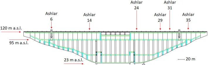
This paper tackles the deformation study of a dam located in Sardinia (Italy) called Eleonora D’Arborea or Cantoniera dam. Waters gathered from Tirso river give rise to the Omodeo lake (see Figure 1), that is one of the largest artificial basin of Europe having a water full capacity of 792.84 Mm3. This huge reservoir supplies drinking water, but it is also used for irrigation and for hydroelectric energy generation. Due to hydrogeological characteristics of the area Cantoniera dam has an original shape. It is a hollow gravity dam with 38 deployed ashlars (each 15 m long and 4 m wide, see Figure 2). The dam is 100 m high and 582 m long, the structure is monitored by 90 extensometers, 122 mono-axial and 4 tri-axial joint-meters. In addition, almost each ashlar has targets for collimation measures and 14 of them are equipped with pendulum chambers, having installed two optical instruments (direct and reverse pendulums with both 0.01 mm accuracy). Recently, also a GNSS monitoring system has been installed.
Figure 2. Front section of the Cantoniera dam and ashlar deployment.
The dam is managed by ENte Acque Sardegna (ENAS) that has contributed to this study providing monitoring data and ancillary information about the dam. In particular, regarding the monitoring data, they refer to three different systems, based on collimators, pendulums and GNSS receivers.
Collimation observations, in a number equal to 158, have been collected over the period January 2004 – April 2017 on a monthly basis. In the frame of dam monitoring, collimation technique allows measuring the relative displacement of targets, located at the top of the dam, along a unique direction geometrically determined and parallel to the upstream-downstream direction.
About pendulum data, 107 observations have been acquired, roughly once a month from July 2006 to April 2017. Displacement measurements provided by the direct and inverted pendulums have been combined, giving a unique observation. This combination provides the displacement between the anchorage point of the inverted pendulum (fixed and with height depending on the depth of the foundation of the ashlar on which it is installed) and the fasten point of the direct pendulum (free to move together with the ashlar on which it is installed at fixed height over the sea level). In the case of the Cantoniera dam, pendulum measurements refer to displacements occurring at 95 m a.s.l. (above sea level) and they have been linearly propagated up to the top of the dam at 120 m a.s.l. Every pendulum measures the displacements along two orthogonal directions, transversal and longitudinal to the dam crest.
As already mentioned above, recently, a GNSS monitoring system has been installed, too. The GNSS network has been materialized through several double-frequency GNSS antennas along the top of the dam (monitoring points) and in the nearby stable areas (reference points). The system is fully automatized and remotely managed by specific software. Three permanent GNSS stations are located on fixed benchmarks outside the dam and six rover stations deployed in correspondence of ashlars 6, 14, 24, 29, 31 and 35 (see Figure 2). Firstly, three GNSS receivers (Leica GMX902) with AX1202GG antennas, were installed on the ashlars number 14, 24 and 35. Their data became available at the beginning of August 2013. The remaining three ashlars were equipped with GNSS receivers during the subsequent year; observations were provided starting from October 2014. Observation frequency is 1 Hz. Positions of the monitoring points were computed on a daily basis with respect to a reference station installed in a stable area few km away from the dam body. GNSS data have been processed with the Leica GNSS Spider software, using a cut-off angle of 15° and broadcast ephemerides, by evaluating static post-processed phase double differences. In such a way, 3D daily coordinates of each monitoring point have been estimated in the WGS84 reference frame.
solutions estimated on these ashlars constitute a time series of about 840 values in the period from October 2014 to April 2017, while for pendulums and collimators, 30 observations are available in the same period. The positions on December 10, 2014 have been considered as the references for the displacements in all the three techniques. The investigations on these time series will be presented in the next section.
3. Time series comparison and modeling
In order to properly compare the data collected with the different techniques, it must be taken into account that, in general, GNSS, pendulums and collimation monitoring systems are installed at different positions. Thus, the observed displacements reflect the dam deformations in different ways. So, in order to compare them, proper reference systems must be defined and data must be reduced to them accordingly. In this paper, it was decided to consider only the GNSS and the pendulum derived observations, which has been made comparable following an approach that is based on the observed data. Collimator data have been only considered in a general discussion in the conclusions, being less accurate and quite sparse in time.
3.1. Defining the reference frames for comparing the GNSS and the pendulum horizontal displacements
For each GNSS station point, a local level reference system has been defined. The origin has been put equal to the average latitude (lat.), longitude (lon.) and ellipsoidal height (h.) of the coordinates estimated in the period from December 10, 2014 to December 9, 2015, the North direction (N) is tangent to the meridian, northward, and the East direction (E) is tangent to the parallel, eastward. Then, the GNSS estimated WGS84 geographic coordinates (lat., lon., h) have been shifted in the (N, E, Up) local coordinates defined on each GNSS station point.
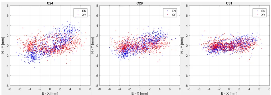
If these (N, E) coordinates are plotted for the three GNSS stations that are in correspondence with the three pendulum devices, placed at ashlars 24, 29 and 31 respectively, they result in clouds of points as it is represented in Figure 3 (blue dots). The three point clouds are roughly distributed as an ellipse having the two semi-axes with different magnitude and orientation, depending on the considered ashlar. Considering the same observation period, the whole dam crest does not move homogeneously. The displacements increase from the eastern dam edge to the center, in fact points are more dispersed for ashlar 24 that is the most central, while the opposite behavior is observed in ashlar 31, close to the constrained edge of the dam.
Then, for each ashlar, the E-N frame has been rotated to an X-Y orthogonal frame having the X axis aligned to the direction of maximum displacement as derived by the observations. The rotation angle between the two reference systems has been evaluated by estimating via Least Square adjustment (LS) the angular coefficient ‘a’ of the straight line model North = a·East. This has been done using one year of data during the same data span used above. The resulting angles αi=arctan(ai) (i=1,2,3) are 28.0°,
Finally, for each GNSS station, the GNSS observed displacements in the East-North frame have been rotated to the corresponding (X,Y) frame (see Figure 3, red dots). It must be stressed that, by applying this procedure, nor the (N,E) neither the (X,Y) system defined in each GNSS station is aligned to the pendulum reference frame. So, in order to compare the displacements from GNSS (X,Y)i=1,2,3 with
those from pendulum, we have to align the pendulum frames to the GNSS (X,Y)i=1,2,3 frames.
Figure 3. Displacements estimated on ashlars 24 (left), 29 (centre) and 31 (right) by GNSS in the East-North (blue dots) and in the X-Y (red dots) reference systems in the period December 10, 2014 to
December 9, 2015
Pendulum data are framed in a local reference system depending on the orientation of the ashlar. Generally, the reading table is mounted so that the two axes T-L are aligned with the Transversal and Longitudinal directions of the ashlar, which are assumed to be parallel to the upstream-downstream direction and to the dam crest direction, respectively.
The (T-L) pendulum displacements in the 24, 29 and 31 ashlars are plotted in Figure 4 (blue dots). Also in the case of pendulum data, the displacements highlight different behaviors in the different ashlars, so that the rotation between each T-L frame and the corresponding (X’,Y’) frame is different. Thus, again, it must be underlined that three different reference systems must be assumed also for the three pendulums. In order to align the (T,L)i=1,2,3 axes to the cross-crest and along-crest directions, a
procedure similar to the one devised for the GNSS coordinates has been adopted.
Figure 4. Displacements observed on ashlars 24 (left), 29 (centre), 31 (right) by pendulums in the T-L(blue dots) and X’–Y’ (red dots) reference systems from December 10, 2014 to December 9, 2015
By adopting this procedure, we assume that the observed pendulum displacements and the observed GNSS displacements refer to reference systems which are pairwise parallel, that is we can consider (X,Y)i parallel to (X’,Y’)i, i=1,2,3.
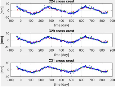
In Figure 5 and Figure 6, the rotated pendulum and GNSS displacements are plotted for ashlars 24, 29, 31 in the cross-crest (X and X’) and along-crest (Y and Y’) directions respectively for the period October 2014 to April 2017.
Figure 5. Displacements estimated on ashlars 24 (top), 29 (centre), 31 (bottom) by pendulums (red dots) and GNSS (blue dots) in the cross-crest direction (green dots represents the collimator
Figure 6. Displacements observed on ashlars 24 (top), 29 (centre), 31 (bottom) by pendulums (red dots) and GNSS (blue dots) in the along-crest direction from October 2014 to April 2017
In the cross-crest direction (Figure 5), the annual periodicity is clearly visible both in pendulums and GNSS displacements. Pendulum and GNSS data are in phase, describing the same oscillations although with slightly different amplitudes. This could be due to the propagation of pendulums data from the height of the measuring camera (at 95m a.s.l.) to the dam crest (at 120m a.s.l.). In fact, a simple linear propagation was applied to the pendulum observed displacements, which is likely to describe the ashlar deformation too roughly. For the along-crest direction the pendulum displacements are negligible, while GNSS detects displacements in the range from 6 mm for ashlar 24 to 4 mm for ashlar 29 and to the noise level when considering ashlar 31. This behavior could be explained again in terms of the inadequate transfer function that has been used in propagating the pendulum displacements, coupled with ashlars positions along the dam structure.
The previous outcomes highlight the specific behaviors of the monitoring techniques here presented. Nominally, GNSS monitoring systems are less accurate than the pendulum measurements but they allow describing the dam displacements with denser observations without losing the capability of detecting periodicity that is typical for this kind of monitoring problem. The higher frequency in the measurement acquisition leads to a better estimate of an analytical model able to properly describe (and predict) the expected displacements.
3.2. Analytical modeling of observed dam deformations
are referred to as ‘deterministic’ models) and one dependent by auxiliary variables as the time t (we will call this method as ‘predictive’ from now on). Both methods have advantages and disadvantages. Models adopting physical parameters directly express the relationship between mechanical properties and dam deformations. However, a reliable and accurate deterministic model is difficult to develop because of the uncertainty and complexity of the dam structure. On the other hand, predictive models completely disregard the dam structure design thus describing the deformations in a purely phenomenological way, although leading to relevant results. This second group of models are simpler and computationally straightforward, and allow predicting the future dam behavior.
We decided to model the pendulum and the GNSS displacements using the predictive model by De Sortis and Paoliani (2007), who proposed a formulation for describing deformation of buttress gravity dams. Other models can be found in Dai et al. 2015, Montillet et al. 2017 and references therein.
Following the selected approach, the crest displacement ∆s can be modeled by a linear trend and two periodic components accounting for annual and semi-annual signals.
Thus, such a model has the following expression:
∆𝑠𝑠=𝑎𝑎+𝑏𝑏 ∙ 𝑡𝑡+𝑐𝑐 ∙cos �2𝜋𝜋𝑇𝑇
1𝑡𝑡�+𝑑𝑑 ∙ 𝑠𝑠𝑠𝑠𝑠𝑠 � 2𝜋𝜋
𝑇𝑇1𝑡𝑡�+𝑒𝑒 ∙cos � 2𝜋𝜋
𝑇𝑇2𝑡𝑡�+𝑓𝑓 ∙ 𝑠𝑠𝑠𝑠𝑠𝑠 � 2𝜋𝜋
𝑇𝑇2𝑡𝑡� (1)
where t is the time expressed in days, T1 is the annual period (365 days) and T2 is the semi-annual
period (T2=T1/2).
The linear term describes potential plastic deformations whereas the harmonic components describe periodic oscillations of the dam crest primarily due to the thermal effects caused by the differences between air and water temperature over the year (the reservoir temperature is lower than the temperature of the air in summer so that the dam moves along the upstream direction, the opposite occurring during winter).
For both GNSS and pendulum data of the three ashlars, model coefficients have been estimated by LS adjustment of the observations in both the cross and along-crest directions. In order to tune the models, a t-test for null hypothesis has been applied on each estimated coefficient, with a 5% significance level.
Fig 7a. Estimated models (red line) and observed displacements (blue dots) in the cross-crest direction by GNSS (left) and pendulums (right)
Fig 7b. Estimated models (red line) and observed displacements (blue dots) in the along-crest direction by GNSS (left) and pendulums (right)
Fig 8b. Residuals of the estimated models in the along-crest direction by GNSS (left) and pendulums (right)
Table 1. Standard deviation of the differences between the observations and the corresponding models
Ashlar Sensor Along-crest Cross-crest
Stand. Dev. [mm]
Stand. Dev. [mm]
no. 24 pendulum 0.08 0.37
GNSS 0.69 0.88
no. 29 pendulum 0.26 0.28
GNSS 0.68 0.80
no. 31 pendulum 0.10 0.23
GNSS 0.67 0.77
The discrepancies between modeled displacements confirm the underestimation of the displacements in the pendulum w.r.t. GNSS.
The statistics of the residuals show that GNSS is less precise than pendulum, which is quite expected. Pendulum residuals have mean standard deviation of 0.22 mm while GNSS residuals mean standard deviation is 0.75 mm. Nevertheless, this proves that GNSS is able to monitor displacements of the order of some millimeters (see Figure 7a and 7b where the model displacements are given).
4. Comments and conclusions
The comparative analyses that have been carried out on pendulum, GNSS and collimator data have shown that pendulum is the most accurate method for estimating the dam deformations. However, this method can be applied only in few points in the dam structure and thus an overall description of these deformations is not possible. Furthermore, the pendulum data are collected inside the dam structure and cannot account properly for crest displacements, which are underestimated as we have shown in our investigations.
GNSS techniques can be profitably used for a precise monitoring of the dam. Although less precise than pendulum, they are accurate enough. Also, GNSS instruments can be deployed on the dam crest and in a larger number than pendulums. This is particularly true nowadays, since low cost receivers can provide high precision positioning (Caldera et al., 2016). Also, GNSS data can be collected in highly automated way and time series can be estimated straightforwardly.
Based on our results, one can say that collimator data are less precise than pendulum and GNSS and should be then replaced in view to have an effective monitoring of the dam displacements. Although one can automate also this technique, this is quite expensive and, most of all, it can suffer for lateral refraction, which can give biased results.
Thus, in the end, we can state that a modern and efficient method for monitoring the displacements in a dam is to integrate some pendulum measurements with a number of GNSS devices placed on the dam crest. In such a way, GNSS observed displacements can be compared and validated with pendulum ones on ashlars where both are present. The deformation analysis can be then densified in other points using GNSS so to have a detailed description of the dam deformations, thus ensuring a reliable estimate of possible anomalous behavior.
Acknowledgements
The authors wish to thank ENAS for kindly supplying the data of the Cantoniera dam and for the subsidiary information allowing the correct interpretation of the results.
References and Notes
1. Alba, M.; Fregonese, L.; Prandi, F.; Scaioni, M.; Valgoi, P. Structural monitoring of a large dam by terrestrial laser scanning. International Archives of Photogrammetry, Remote Sensing and Spatial Information Sciences, 2006, 36(5), 6.
2. Anghel, A.; Vasile, G.; Boudon, R.; d’Urso, G.; Girard, A.; Boldo, D.; Bost, V. Combining spaceborne SAR images with 3D point clouds for infrastructure monitoring applications. ISPRS Journal of Photogrammetry and Remote Sensing, 2016, 111, 45-61.
3. Antova, G. 3d Laser Scanning for Dam Deformation Monitoring. In 7th International Scientific Conference-SGEM2007, 2007, SGEM Scientific GeoConference.
5. Behr, J.; Hudnut, K.; King, N. Monitoring structural deformation at Pacoima dam, California using continuous GPS. In Proc. of ION GPS, September 15-18, 1998, Vol. 11, 59-68.
6. Caldera, S.; Realini, E.; Barzaghi, R.; Reguzzoni, M.; Sansò, F. Experimental study on low-cost satellite-based geodetic monitoring over short baselines. Journal of Surveying Egineering (ASCE),
2016, 142(3).
7. Chrzanowski, A.; Szostak-Chrzanowski, A. Deformation monitoring surveys-old problems and new solutions. Reports on Geodesy, 2009, 85-103.
8. Dai, W.; Huang, D.; Liu, B. A phase space reconstruction based single channel ICA algorithm and its application in dam deformation analysis. Survey Review, 47(345), 2015, 387-396.
9. Dardanelli, G.; La Loggia, G.; Perfetti, N.; Capodici, F.; Puccio, L.; Maltese, A. Monitoring displacements of an earthen dam using GNSS and remote sensing. SPIE Remote Sensing, 2014, 923928-923928.
10. De Loach, S. R. Continuous deformation monitoring with GPS. Journal of Surveying Engineering, 115(1), 1989, pp.93-110.
11. De Sortis, A. ; Paoliani, P. Statistical analysis and structural identification in concrete dam monitoring. Engineering Structures, Vol. 29, Issue 1, January 2007, 110-120.
12. Di Martire, D.; Iglesias, R.; Monells, D.; Centolanza, G.; Sica, S.; Ramondini, M.; Pagano, L.; Mallorquí, J. J.; Calcaterra, D. Comparison between differential SAR interferometry and ground measurements data in the displacement monitoring of the earth-dam of Conza della Campania (Italy). Remote sensing of environment, 2014, 148, 58-69.
13. Drummond, P. Combining CORS Networks, Automated Observations and Processing, for Network Rtk Integrity Analysis and Deformation Monitoring. Proceedings, 15th FIG Congress Facing the Challenges – Building the Capacity, Sydney, 2010, Australia.
14. Galán-Martín, D.; Marchamalo-Sacristán, M.; Martinez-Marín, R.; Sánchez-Sobrino, J. A. Geomatics applied to dam safety DGPS real time monitoring. International Journal of Civil Engineering, 11, 2010, 134-141.
15. Honda, K., Nakanishi, T.; Haraguchi, M.; Mushiake, N.; Iwasaki, T.; Satoh, H.; Kobori, T.; Yamaguchi, Y. Application of exterior deformation monitoring of dams by DInSAR analysis using ALOS PALSAR. In Geoscience and Remote Sensing Symposium (IGARSS), 2012, IEEE International, 6649-6652.
16. Mascolo, L.; Nico, G.; Di Pasquale, A.; Pitullo, A. Use of advanced SAR monitoring techniques for the assessment of the behaviour of old embankment dams. In Earth Resources and Environmental Remote Sensing/GIS Applications V, vol. 9245, 2014, p. 92450N. International Society for Optics and Photonics.
17. Milillo, P.; Perissin, D.; Salzer, J. T.; Lundgren, P.; Lacava, G.; Milillo, G.; Serio, C. Monitoring dam structural health from space: Insights from novel InSAR techniques and multi-parametric modeling applied to the Pertusillo dam Basilicata, Italy. International Journal of Applied Earth Observation and Geoinformation, 2016, 52, 221-229.
18. Montillet, J. P., Szeliga, W. M., Melbourne, T. I., Flake, R. M., Schrock, G. Critical Infrastructure Monitoring with Global Navigation Satellite Systems. Journal of Surveying Engineering, 142(4),
19. Radhakrishnan, N. Application of GPS in structural deformation monitoring: A case study on Koyna dam. Journal of Geomatics, 2014, 8(1).
20. Rutledge, D. R.; Meyerholtz, S. Z.; Brown, N.; Baldwin, C. Dam stability: Assessing the performance of a GPS monitoring system. GPS World, 2006, 17(10), 26–33.