Quantum Key Recycling with eight-state encoding (The Quantum One Time Pad is more interesting than we thought)

Quantum Key Recycling with eight-state encoding

Boris ˇ

Skori´

c and Manon de Vries

Abstract

Perfect encryption of quantum states using the Quantum One-Time Pad (QOTP) requires 2 classical key bits per qubit. Almost-perfect encryption, with information-theoretic security, requires only slightly more than 1. We slightly improve lower bounds on the key length. We show that key lengthn+2 log1

ε suffices to encryptnqubits in such a way that the cipherstate’s L1-distance from uniformity is upperbounded byε. For a stricter security definition involving the∞-norm, we prove sufficient key lengthn+ logn+ 2 log1

ε+ 1 + 1 nlog

1 δ+ log

ln 2

1−ε, whereδ is a small probability of failure. Our proof uses Pauli operators, whereas previous results on the∞-norm needed Haar measure sampling.

We show how to QOTP-encrypt classical plaintext in a nontrivial way: we encode a plaintext bit as the vector±(1,1,1)/√3 on the Bloch sphere. Applying the Pauli encryption operators results in eight possible cipherstates which are equally spread out on the Bloch sphere. This encoding, especially when combined with the half-keylength option of QOTP, has advantages over 4-state and 6-state encoding in applications such as Quantum Key Recycling and Unclon-able Encryption. We propose a key recycling scheme that is more efficient and can tolerate more noise than a recent scheme by Fehr and Salvail.

For 8-state QOTP encryption with pseudorandom keys we do a statistical analysis of the cipherstate eigenvalues. We present numerics up to 9 qubits.

1

Introduction

1.1

Quantum encryption and key recycling

Quantum physics is markedly different from classical physics regarding information processing. For instance, performing a measurement on an unknown quantum state typically destroys state information. Furthermore, it is impossible to clone an unknown state by unitary evolution [1]. These two properties are very interesting for security applications, since they provide a certain amount of inherent confidentiality, unclonability and tampering detection. Quantum physics also has entanglement of subsystems, which allows for feats like teleportation [2, 3] that have no classical analogue. The laws of quantum physics have been exploited in numerous security schemes, such as Quantum Key Distribution [4, 5, 6], quantum anti-counterfeiting [7], quantum Oblivious Transfer [8, 9], authentication and encryption of quantum states [10, 11, 12], unclonable encryption [13], quantum authentication of PUFs [14, 15], and quantum-secured imaging [16], to name a few. A recent overview of quantum-cryptographic schemes is given in [17].

In this paper we focus on two features that distinguish quantum channels from classical channels: (i) The possibility of achieving almost-perfect encryption of quantum states, with information-theoretic security guarantees, using a key length that is slightly more than half of the length re-quired for perfect encryption. Perfect encryption, e.g. using the Quantum One Time Pad (QOTP), requires a key of length 2nto encryptnqubits. Dickinson and Nayak [18] showed that key length

n+ 2 log1_ε+ 4 suffices if one only requires that the cipherstate is at most εaway from the fully mixed state, in terms of theL1-norm. Aubrun [19] showed that, for a more strict security notion

based on the_∞-norm, key lengthn+ 2 log1_ε+ log 150 suffices.

transmission is successful. Damg˚ard, Pedersen and Salvail [20, 21] introduced a scheme in which theentire key can be re-used. However, encryption and decryption require a quantum computer with circuit depth_O(n2_{) [22]. Fehr and Salvail [23] recently proposed a scheme which re-uses the}

entire key and which does not need a quantum computer.

1.2

Contributions and outline

We present a number of new results regarding the use of the QOTP.

• We introduce a new way of encoding a classical bit as a qubit state. The ‘0’ is encoded as the vector (1,1,1)T/√3 on the Bloch sphere, and the ‘1’ as the opposite vector (−1,−1,−1)T/√3. By acting with the four QOTP encryption operators on our two plaintext states we obtain eight cipherstates that are equally spread out on the Bloch sphere. We refer to this encoding as ‘8-state encoding’.

• We propose a key recycling scheme inspired by [23], but using 8-state encoding. Our scheme is more compact by virtue of the fact that 8-state encoding is a proper encryption, while 4-state and 6-state encoding are leaky. Furthermore our scheme tolerates more noise.

• We study the use of the QOTP with a pseudorandom key, for general states. We model the pseudorandomness as the output of a random function. For n qubits and key length q, we construct a random tableT of size 2q

×n, where thej’th row is the key corresponding to seedj. The adversary knowsT but not the row indexj.

Using this model we show that key lengthn+ 2 log1

ε suffices to encryptnqubits in such a way that the cipherstate’sL1-distance from uniformity is upperbounded byε. Our bound is slightly

tighter than Dickinson and Nayak’s result [18]. For a more strict security property based on the_∞-norm we prove sufficient key lengthn+ logn+ 2 log1

ε+ 1 +

1

nlog

1

δ + log

ln 2

1−ε, whereδ is the failure probability. Similar expressions are known in the literature [27, 19] (even without the lognterm). However, those results needed the encryption operators to be drawn from the Haar measure.

• We study the pseudorandom-keyed QOTP in the case of 8-state encoding of classical plaintexts. We derive bounds on the moments of the cipherstate eigenvalues; these bounds are sharper than for arbitrary states. We present numerics that show a ‘phase transition’ as the key length crosses over fromq < nto q > n.

The outline is as follows. In Section 2 we briefly review the QOTP and security definitions for quantum ciphers. In Section 3 we introduce 8-state encoding and examine its properties. A comparison is given with 4-state and 6-state encoding, regarding conditional entropies of plaintexts and keys. In Section 4 we present our Key Recycling scheme and discuss its security properties. In Section 5 we briefly mention two other possible applications of 8-state encoding: Unclonable Encryption with shorter keys, and the three-pass keyless protocol.

The pseudorandom-keyed QOTP results for general states are given in Section 6. In Section 7 we restrict the states to 8-state encoding.

2

Preliminaries

2.1

Notation and terminology

Classical Random Variables (RVs) are denoted with capital letters, and their realisations with lowercase letters. The probability that a RV X takes value x is written as Pr[X = x]. The expectation with respect to RVX is denoted asExf(x) =Px∈XPr[X =x]f(x). Sets are denoted in calligraphic font. The notation ‘log’ stands for the logarithm with base 2. The min-entropy of

X _{∈ X} isHmin(X) =−log maxx∈XPr[X =x], and the conditional min-entropy is Hmin(X|Y) = −logEymaxx∈XPr[X =x|Y =y]. The notationhstands for the binary entropy functionh(p) =

plog1

p+ (1−p) log

1

For quantum states we use Dirac notation, with the standard qubit basis states|0iand |1i rep-resented as 1₀and 0₁respectively. The Pauli matrices are denoted as σx, σy, σz, and we write

σ = (σx, σy, σz). The standard basis is the eigenbasis of σz, with|0iin the positivez-direction. We write 1d for thed×didentity matrix. The fully mixed state ind-dimensional Hilbert space is denoted as τd = 1_d1d, or simply τ if the dimension is clear from the context. The space of mixed state operators acting on Hilbert space _His written as_S(_H). The 1-norm of an operator

Awith eigenvaluesλi is defined as|A|1= tr|L|=Pi|λi|. The notation ‘tr’ stands for trace. The statistical distance (trace distance) between two mixed states is defined asD(ρ, ρ0_{) =} 1

2tr|ρ−ρ0|.

The_∞-norm_|A_|∞ is maxi|λi|.

We will use the Positive Operator Valued Measure (POVM) formalism. Consider a bipartite system ‘AB’ where the ‘A’ part is classical, i.e. the state is of the form ρAB _=E

x∈X|xihx| ⊗ρBx with the|xiforming an orthonormal basis. The min-entropy of the classical RVX given part ‘B’ of the system is [24]

Hmin(X|ρBX) =−log max

M Ex∈XtrMxρ B

x. (1)

Here _Mdenotes a POVM, i.e. _M= (Mx)x_∈X where the operatorsMx are positive semidefinite and satisfyP_x∈XMx=1. Let Λ

def

= P_xρB

xMx. The POVM which achieves the maximum in (1) satisfies the necessary and sufficient conditions Λ†_{= Λ and∀}

x: Λ−ρBx ≥0.

2.2

The Quantum One Time Pad

An arbitrary unknown qubit state can be perfectly encrypted using a classical two-bit key [12, 25, 26]. The simplest way of doing this is using the Quantum One-Time Pad (QOTP). Consider a pure state |ψiand let the key be (u, w)∈ {0,1}2_{. The encrypted state is |ψ}

uwi=Euw|ψi, with

Euw the unitary encryption operator, Euw = |wih0|+ (−1)u|1⊕wih1|. In terms of Pauli spin matrices: E00=1,E01=σx, E10=σz,E11=σxσz.

Euw=σwxσzu. (2) For notational brevity we will often write the key asb= 2u+w,b _{∈ {}0,1,2,3_} and accordingly encryption operatorEb and cipherstate|ψbi=Eb|ψi. From the point of view of an attacker Eve who does not know u, w, the qubit is in the fully mixed state: 1

4

P

b|ψbihψb| = 1₂12. In other

words, from Eve’s point of view the cipherstate carries no information at all aboutψ. For a mixed qubit stateρ the cipherstate isEbρE†b and it holds that

1 4

P

bEbρEb† =

1

212. Any Hilbert space Hdof dimensiond= 2n can be interpreted as ann-qubit system. QOTP encryption onHd works by encrypting every qubit individually. The key is b _{∈ {}0,1,2,3}n_{. The encryption operator} factorises as Eb =Nn_i=1Ebi. From Eve’s point of view the encryption of a state ρ∈ S(Hd) is fully mixed,

∀ρ∈S(H2n)

1 4n

X

b∈{0,1,2,3}n

EbρEb† = (τ2)⊗ n_=τ

2n. (3)

2.3

Security definitions for quantum ciphers

The performance of a quantum cipher can be quantified in several ways. We first consider encryp-tion of generic mixed states.

Definition 2.1 (From [27]) A completely positive, trace-preserving mapR:S(Hd)→ S(Hd)is calledε-randomising if

∀ϕ∈S(Hd): |R(ϕ)−τd|∞≤ ε_d. (4)

in the stateEk∈KEx∈X|kihk| ⊗ |xihx| ⊗ρk,x. Eve has access only to the third part, and her main interest is in the second part. Tracing out the first subsystem gives the bipartite state

ρ=Ex∈X|xihx| ⊗ρx, ρx=Ek∈Kρk,x. (5) We introduce the notation

ξdef= Ex∈Xρx. (6) Typicallyξ=τd. Eve’s knowledge about the plaintext is related to the statistical distance between

X and the uniform distribution, given the quantum stateρX for unknownX. This is written as

d(X|ρX)def= D(ρ, τX⊗ξ) =Ex∈XD(ρx, ξ). (7) If the encryption depends on some public randomness Y _{∈ Y}, then we write ρx(y), and (7) generalises to

d(X_|Y, ρX(Y)) =Ex∈XEy∈YD(ρx(y), ξ). (8)

Definition 2.2 A symmetric quantum cipher is called “statisticallyε-private” [20] or “a scheme with errorε” [13] if

∀x,x0_∈X : D(ρx, ρx0)< ε. (9) We introduce a security definition inspired by the conditional statistical distance (8).

Definition 2.3 Let Ry : S(Hd) → S(Hd) be a completely positive trace-preserving map, with

y∈ Y public. The map is called “ε-uniform” if it satisfies

∀ϕ∈S(Hd): Ey∈YD(Ry(ϕ), τd)≤ε. (10)

A symmetric quantum cipher for classical messages which makes use of public randomnessY _{∈ Y}

is called “ε-uniform” if it satisfies

∀x∈X : Ey∈YD(ρx(y), ξ)≤ε. (11)

We introduce Def. 2.3 because the properties (10,11) appear in the literature (without the condi-tioning onY) but receive either no name or a confusing name. We will use Def. 2.3 in Section 6. Beingε-randomising (Def. 2.1) implies being ε₂-uniform (Def. 2.3 with deterministicy). Similarly, a cipher satisfying Def. 2.2 also satisfies Def. 2.3. Note that (11) impliesd(X_|ρX)_≤ε.

When the key is chosen completely at random, the QOTP has parameterε= 0 in all the above definitions.

Below we list a number of results on almost-perfect quantum encryption that can be found in the literature. The cipherstate is denoted asρ∈ S(H2n).

Security property Key length Comment

[27] Thm. II.2 |ρ−τ|∞≤ 2εn n+ logn+ 2 log1_ε+ log 134 Haar [19] Thm. 1 _|ρ₋τ_|∞≤ ε

2n with nonzero prob. n+ 2 log1_ε+ log 150 Haar [27] Thm. A.3 |ρ−τ|1≤ε n+ logn+ 2 log1_ε Pauli

[18] Thm. 1.2 _|ρ₋τ_|1≤ε n+ 2 log1_ε+ 4 Pauli

‘Haar’ indicates that the encryption operators are drawn according to the Haar measure (which is considered to be difficult). ‘Pauli’ means that Pauli operators are used.

3

Eight-state encoding

It has been remarked in the literature that applying the Quantum One Time Pad to classical data is not very exciting: Acting with any encryption operatorEuwon|0ior|1iyields either|0ior|1i, and hence the QOTP does the same as the classical OTP except it needs twice the key material. Furthermore, the quantum encryption yields no protection against copying of the cipherstates.

This is the case only when the basis for representing a classical bit is chosen badly.

We propose a basis such that QOTP encryption of a classical bit is nontrivial, resulting in 8 dif-ferent cipherstates which are equally spread out over the Bloch sphere. Although 8-state encoding is very simple and has interesting properties, we are not aware that it has ever been used.

3.1

Equally separated cipherstates

We define cosαdef= 1/√3,α≈0.96.1 _{We write}√_i=eiπ/4_{. We encode the classical ‘0’ and ‘1’ as}

qubit statesψ0, ψ1,

|ψ0i def

=

_cosα

2 √

i sinα₂

|ψ1i def

=

_sinα

2 −√i cosα₂

hψ1|ψ0i= 0 (12)

which on the Bloch sphere corresponds to the normal vectors (1,1,1)T_/√_{3 and (}

−1,₋1,₋1)T_/√₃

respectively. In spherical coordinates (θ, ϕ) this corresponds to (θ, ϕ) = (α,π₄) and (θ, ϕ) = (π₋α,₋3₄π). Compactly written in terms of the standard basis_|0_i,_|1_i,

|ψgi= (−

√

i)gcosα

2|gi+ ( √

i)1−gsinα

2|1−gi g∈ {0,1}. (13)

We act on these two states with the four encryption operators Euw and obtain eight different cipherstates,

|ψuwgi

def

= Euw|ψgi= (−1)gu h

(₋√i)gcosα_2|g_⊕w_i+ (₋1)u(√i)1−gsinα_2|g_⊕w_ii. (14) On the Bloch sphere these correspond to unit-length vectorsnuwg as follows (see Fig. 1),

nuwg= (₋1)g

√

3  (−1)

u

(₋1)u+w (−1)w



. (15)

The relation between the Bloch sphere anglesθ, ϕand the elliptic polarisation parametersβ (angle from thex-axis to the major axis) and tanζ(ratio minor/major, withζ <0 left rotating) is given by

cosθ= cos 2ζcos 2β ; sinϕ= sin 2ζ/p1₋(cos 2ζcos 2β)2

tan 2β = cosϕtanθ ; sin 2ζ= sinθsinϕ. (16) Our eight cipherstates have β ∈ {±π

8,± 3π

8 }, ζ = ±(

π

4 −

α

2) ≈ ±0.308. We will often write

b= 2u+w,b_{∈ {}0,1,2,3_}as a basis index, with corresponding notationEb,_|ψbgi,nbg.

u w g x y z θ ϕ β ζ cipherstate|ψuwgi

0 0 0 + + + α π/4 π/8 + cosα

2|0i+ √

isinα

2|1i

0 1 0 + _{− −} π₋α ₋π/4 3π/8 ₋ cosα

2|1i+ √

isinα

2|0i

1 0 0 − − + α −3π/4 −π/8 − cosα₂|0i −√isinα₂|1i

1 1 0 ₋ + ₋ π₋α 3π/4 ₋3π/8 + cosα

2|1i − √

isinα

2|0i

0 0 1 _{− − −} π₋α ₋3π/4 ₋3π/8 ₋ sinα

2|0i − √

icosα

2|1i

0 1 1 − + + α 3π/4 −π/8 + sinα₂|1i −√icosα₂|0i

1 0 1 + + ₋ π₋α π/4 3π/8 + sinα

2|0i+ √

icosα

2|1i

1 1 1 + ₋ + α ₋π/4 π/8 ₋ sinα_2|1_i+√icosα_2|0_i

1_sinα=p

2/3; tanα=√2; cosα₂ =q1₂+₂√1

3; sin α 2 =

q₁

2− 1 2√3; tan

α 2 =

√

3−1

√

B. ˇSkori´c 7

E00| 0i

E11| 0i

E01| 0i

E10| 0i

Fig. 2.Relation between the codesCandD?_⇢C..

We thank Christian Scha↵ner, Serge Fehr and Andreas H¨ulsing for useful discussions.

References

1. W.K. Wootters and W.H. Zurek. A single quantum cannot be cloned.Nature, 299:802–803, 1982. 2. C.H. Bennett, G. Brassard, C. Cr´epeau, R. Jozsa, A. Peres, and W.K. Wootters. Teleporting an unknown quantum state via dual classical and Einstein-Podolsky-Rosen channels.Phys. Rev. Lett., 70:1895–1899, 1993.

3. D.N. Matsukevich and A. Kuzmich. Quantum state transfer between matter and light. Science, 306(5696):663–666, 2004.

4. C.H. Bennett and G. Brassard. Quantum cryptography: Public key distribution and coin tossing.

IEEE International Conference on Computers, Systems and Signal Processing, pages 175–179, 1984.

5. A.K. Ekert. Quantum cryptography based on Bell’s theorem.Phys. Rev. Lett., 67:661 – 663, 1991. 6. D. Gottesman and J. Preskill. Quantum Information with Continuous Variables, chapter Se-cure quantum key exchange using squeezed states, pages 317–356. Springer, 2003. arXiv:quant-ph/0008046v2.

7. C.H. Bennett, G. Brassard, S. Breidbard, and S. Wiesner. Quantum cryptography, or unforgeable subway tokens. InCRYPTO, pages 267–275, 1982.

8. I.B. Damg˚ard, S. Fehr, L. Salvail, and C. Scha↵ner. Cryptography in the bounded quantum-storage model. InIEEE Symposium on Foundations of Computer Science (FOCS), page 449, 2005.

9. C. Scha↵ner. Simple protocols for oblivious transfer and secure identification in the noisy-quantum-storage model.Phys.Rev.A, 82:032308, 2010.

10. H. Barnum, C. Cr´epeau, D. Gottesman, A. Smith, and A. Tapp. Authentication of quantum messages. InIEEE Symposium on Foundations of Computer Science, pages 449–458, 2002. Full version athttp://arxiv.org/abs/quant-ph/0205128.

11. P.O. Boykin and V. Roychowdhury. Optimal encryption of quantum bits.Phys.Rev.A, 67:042317, 2003.

12. A. Ambainis, M. Mosca, A. Tapp, and R. De Wolf. Private quantum channels. InIEEE Symposium on Foundations of Computer Science (FOCS), pages 547–553, 2000.

13. B. ˇSkori´c. Quantum Readout of Physical Unclonable Functions.International Journal of Quantum Information, 10(1):1250001–1 – 125001–31, 2012.

14. S.A. Goorden, M. Horstmann, A.P. Mosk, B. ˇSkori´c, and P.W.H. Pinkse. Quantum-Secure Au-thentication of a physical unclonable key.Optica, 1(6):421–424, Dec. 2014.

Figure 1: The eight cipherstates_|ψuwgi=Euw|ψgi shown (left) on the Bloch sphere, forming the

corner points(±1,±1,±1)/√3 of a cube; and (right) as elliptic polarisation states. ‘R’ stands for righthanded, ‘L’ for lefthanded.

3.2

Some properties of eight-state encoding

It holds thathψb0|ψb1i= 0, i.e. opposite bit values encrypted with the same key lead to orthogonal

cipherstates. This trivially follows from the unitarity of the encryption operators, hψb0|ψb1i = hψ0|Eb†Eb|ψ1i=hψ0|ψ1i= 0.

More generally, we can readily compute the inner products between all the various cipherstates from the general rule_|hψb0g0|ψbgi|2= 1₂+1₂nb0g0·nbg,

|hψb0g0|ψbgi|2=δbb0·δgg0 + (1−δbb0) h

δgg01

3+ (1−δgg0) 2 3 i

. (17)

In words: When g gets encrypted with two different keys the two cipherstates have (squared) inner product 1/3; any encryption of g, g0_{, g}0 _{6= g, with unequal keys yields cipherstates that} have (squared) inner product 2/3. The squared inner product determines the probability that one cipherstate gets projected onto another when a projective measurement is performed. Eq. (17) tells us that the nontrivial encryptions of_|ψ1−gilook more like|ψgithan the nontrivial encryptions of

|ψgiitself.

The phases of the inner products_hψu0w0g0|ψuwgiare given by

hψu0w0g0|ψuwgi

i(u0₋u)(w0+w)₍₋₁₎δ3,u0+u+w0+w = δgg

0δ_uu0δ_ww0+δ_gg0(1−δ_uu0δ_ww0)(−1) g

√

3 +δgg0

r 2 3

n

δww0δuu0−δww0exp h

(g−g0)(−1)u+u0iπ

3 io

. (18) Table 1 gives a comparison of four-, six-, and eight-state encoding regarding the entropy of the classical variablesGandB given that an attacker Eve holds the qubit (‘E’). Table 2 contains the same information but lists entropylosses.

The states in 4-state encoding are the eigenstates ofσz andσx. In 6-state encoding one uses the eigenstates ofσz, σx andσy. Let the random variableM denote the outcome of a measurement (possibly POVM) on the qubit E. In the 4-state case, the measurement that minimisesH(G_|M) and Hmin(G|M) is the projective measurement σx +σz; the H(B|GM) and Hmin(B|GM) are

minimised by measuringσx−σz.

In the 6-state case, H(G|M) and Hmin(G|M) are minimised by measuring σx+σy +σz; the H(B_|GM) by the POVM _{M_b(g)_}3

b=1, Mb = 1₃1+ 1₃(−1)gnb ·σ, n1 = (−2,1,1)T/ √

6, n2 =

(1,₋2,1)T_/√_6,n

3= (1,1,−2)T/√6; theHmin(B|GM) is minimized by the POVM ‘opposite’ to

the one above, i.e. withnb→ −nb.

In the 8-state case, the H(B_|GM) is minimised by the POVM M_b(g) = 1

2|ψbgihψbg| and the

Table 1: Conditional Shannon entropies and min-entropies

4-state 6-state 8-state

H B|E 1 log 3≈1.585 2

G|E h(cos2 π

8)≈0.601 h(cos

2α

2)≈0.744 1

B|GE h(cos2 π

8)≈0.601 H( 1−2/√6

3 , 1+1/√6

3 , 1+1/√6

3 )≈1.271 log 3

G|BE 0 0 0

BG|E 3

2 log 3 +

2

3 ≈2.252 3 2+

3

4log 3≈2.689

Hmin B|E 1 log 3 2

G|E −log cos2π

8 ≈0.228 −log cos

2α

2 ≈0.342 1

B|GE −log cos2π₈ ≈0.228 −log(1₃ +₃√2

6)≈0.724 1

G|BE 0 0 0

BG|E 1 log 3 2

Table 2: Entropy losses

4-state 6-state 8-state

H(G)₋H(G_|E) 0.399 0.256 0 H(B)₋H(B_|GE) 0.399 0.314 0.415 H(BG)₋H(BG_|E) 1

2

1

3 0.311

Hmin(G)−Hmin(G|E) 0.772 0.658 0

Hmin(B)−Hmin(B|GE) 0.772 0.861 1

In all encodings (4,6,8) the H(BG_|M) and Hmin(BG|M) are minimised by the POVM {Mbg}bg with Mbg = _#bases1 |ϕbgihϕbg|, where|ϕbgi denotes the encoding of bit value g in basis b. In all encodings we find thatHmin(G|BE) = 0;Hmin(B|E) =Hmin(B);Hmin(BG|E) =Hmin(B).

Another important property is the intercept-resend disturbance probability. Let Alice send _|ϕbgi for randomb, g. Eve does a projective measurement in any basis and forwards the outcome_|χ_ito Bob. Bob measures_|χ_iin basisb. Averaged overb andg, Bob’s probability of getting the wrong outcome (g) is 1/4 in the case of 4-state encoding and 1/3 for 6-state and 8-state.

In Section 4 we will be interested in (i) hiding G and (ii) hiding B when the plaintext G is known. In Table 2 we see that 8-state encoding does a better job of ensuring these two things simultaneously than 4-state and 6-state.

4

Key Recycling

When Alice and Bob have a (one-way) quantum channel at their disposal and an authenticated two-way classical channel, they can achieve unconditionally secure communication by using Quantum Key Distribution (QKD) and then applying a classical One Time Pad (OTP). This has been well known since the first work on quantum cryptography.

4.1

Requirements for Key Recycling; state of the art

Consider anm-bit message encoded inn qubits (withn > m), using a keyk. A Quantum Key Recycling (QKR) scheme typically needs to refreshnbits of key material if Bob detects tampering (“reject”), and a much smaller amountt,tn, possibly t= 0, if Bob does not detect tampering (“accept”). Loosely speaking a QKR scheme has to satisfy the following requirements.

R1 If Eve steals the entire cipherstate, the message must remain secret.

R2 If Eve knows the entire plaintext and Bob accepts, Eve does not learn more than t+εbits of information about the key, whereεis negligible.

If Bob accepts, the key update mechanism computes a new keyk0_{from the old keykandtbits of} fresh key material unknown to Eve. This makes sure that Eve has negligible knowledge about the new keyk0_{. If Bob rejects, the worst case assumption is that Eve has stolen the entire cipherstate} and already knew the plaintext. Eve then could in principle learn up ton key bits. Hence Alice and Bob have to introducenfresh key bits in the next encryption.

Damg˚ard et al. [20, 21] introduced a QKR scheme witht= 0, for a noiseless quantum channel. A classical authentication tag is first attached to the message; this is then classically on-time-padded; finally quantum encryption is performed by selecting a basis from a set of 2n _{Mutually Unbiased} Bases (MUBs). The scheme is elegant but has the drawback that it needs a quantum computer with circuit depth_O(n2_{) [22] for the encryption and decryption.}

Fehr and Salvail [23] recently proposed a QKR scheme that works with individual BB84 qubits, without needing a quantum computer. It hast= 0. However, it tolerates very little noise.

4.2

Proposed QKR scheme #1

We first propose a QKR scheme which is essentially a copy of [23] but using QOTP encryption.2

The message is µ_{∈ {}0,1_}`_{. The scheme makes use of an extractor Ext:}

{0,1_}n

→ {0,1_}` _and a keyed hash function (MAC)M that produces an authentication tag of lengthλ. The security parameter isλ. The hash function must have the special property of beingmessage-independent, i.e. the distribution ofM(K, µ) does not depend on the messageµ. Furthermore the hash function must have key privacy, i.e. an attacker with limited information about µ learns almost nothing about the key. (These notions are explained in [23], and it turns out that implementation is straightforward.)

The scheme needs a second keyed hashSS which too is message-independent and key-private; it is used as a Secure Sketch. A Secure Sketch is a secure form of error correction. Given a sketch SS(k, x) of a message x, and a noisy version x0, it is possible to recover x. Secure Sketches with message independence and key privacy were discussed in [36]. Though constructions exist, they do not tolerate much noise.

The key material consists of three parts: KMAC for MAC-ing; KSS for the secure sketch; and

b_{∈ {}0,1,2,3_}n _{being QOTP bases.} Encryption

Generate random x_{∈ {}0,1_}n_{. Compute s=SS(K}

SS, x) and z=Extx. Compute the ciphertext

c = µ_⊕z and authentication tag T = M(KMAC, x||c||s). Prepare the quantum state |Ψi =

Nn

i=1|ψbixii. Send|Ψi,s,c,T. Decryption

(The recipient gets|Ψ0i,s0,c0,T0.)

Measure|Ψ0i in the b-basis. This yields x0 ∈ {0,1}n_{. From x}0_{, s, K}

SS recover ˆx, an estimator

forx. Compute ˆz=Extxˆ and ˆµ=c0⊕ˆz. Accept the message ˆµif thex-recovery succeeded and

T0=M(KMAC,xˆ||c0||s0).

Key update

In case of Accept, re-use the entire key. In case of Reject, compute the updated keyb0_{as a function} ofbandnfresh secret bits.

4.3

Analysis of QKR scheme #1

The modification w.r.t. the scheme of Fehr and Salvail is small but has a significant effect. In the original scheme [23], the 4-state encoding causes leakage aboutx; this necessitates a large amount of compression3_{byExtin order to keepµsecure (Requirement R1). In the case of 8-state encoding}

much less compression is needed. Compression is needed primarily because of the channel noise. It is prudent to assume that all noise is caused by Eve. Eve may steal whole qubits from|Ψior extract information into ancillas. This gives hernf(β) +abits of information aboutx, wheref(β) is an increasing function4 _{of the bit error rate β, with f(0) = 0,f(}1

2) = 1, anda is a constant

independent ofn. Eve’s uncertainty aboutxgivenzisn−`bits; this has to cover thenf(β) +a. Hence we have to set`≤n[1−f(β)]−a.

Note that asymptotically (n_{→ ∞}) the constantabecomes negligible. In the caseβ 1 we see that asymptoticallythe number of qubits nneeded to send the`-bit message is just slightly larger than`.

4.4

Proposed QKR scheme #2

Scheme #1 has very limited noise tolerance due to the fact that it needs a special Secure Sketch with message independence and key privacy. We will now loosen this restriction and work with an ordinary Secure SketchS, for instance a syndrome of an error-correcting code. The price to pay is that the sketchS(x), if sent in plaintext, leaks aboutx. If the sketch is sent encrypted with key

KSSand Eve knowsµ, then the sketch leaks information aboutKSS. We choose the second option

and accept that KSS has to be updated even if Bob accepts. We set the length ofKSS equal to

the length ofS(x), which asymptotically approachesnh(β). Encryption

Generate randomx_{∈ {}0,1_}n_{. Computes=K}

SS⊕S(x) andz=Extx. Compute the ciphertext

c = µ_⊕z and authentication tag T = M(KMAC, x||c||s). Prepare the quantum state |Ψi =

Nn

i=1|ψbixii. Send|Ψi,s,c,T. Decryption

(The recipient gets_|Ψ0_i,s0_,c0_,T0_.)

Measure_|Ψ0_{iin the b-basis. This yieldsx}0 _{∈ {0,1}}n_{. Recover ˆxfromx}0 _andK

SS⊕s0. Compute

ˆ

z = Extxˆ and ˆµ = c0 ⊕ˆz. Accept the message ˆµ if the syndrome decoding succeeded and

T0=M(KMAC,xˆ||c0||s0).

Key update

If Bob accepts, replace KSS. If Bob rejects, replace KSS and compute the updated key b0 as a

function ofbandnfresh secret bits.

4.5

Analysis of QKR scheme #2

The security of scheme #2 is the same as for #1. The one-time-padded sketch reveals no informa-tion aboutx; this is the same situation as with the special functionSS. We now have a primitive with the following asymptotics:

• It securely sends an `-bit classical message while using up only nh(β) = `₁₋h_f(β₍)_β) bits of key material.

• It works as long asf(β)<1.

• It uses up less key material than a classical OTP as long as ₁₋h(_fβ₍)_β) <1, i.e. 1−f(β)−h(β)>0. The condition 1₋f(β)₋h(β)>0 is similar to the noise condition under which qubit-based QKD is possible. Whenever qubit-based QKD is possible, scheme #2 works and is a better alternative than repeated use of QKD and classical OTP.

3_{n≈(1−0.772)}−1_{`≈4.3`(see line 4 of Table 2) to compensate the min-entropy loss.}

4_{If Eve steals and stores 2β qubits from|Ψi, she causes bit error rateβ. By repeatedly stealing qubits which}

have been encrypted with the same keybi, Eve would essentially learn the plaintext valuesxi. From the existence

4.6

Proposed QKR scheme #3

We apply the above discussed primitive to itself: Instead of sending the OTP’ed sketch s =

KSS⊕S(x) as an ordinary classical message, we send sas a payload using scheme #2.

We denote quantities in the original primitive with label ‘0’ and in the additional part with ‘1’. We have µ1 =s0. The additional keys and classical/quantum transmissions required for this action

(asymptotically) are listed below.

• A basis keyb1∈ {0,1,2,3}n1. A keyKSS(1)∈ {0,1}n1h(β).

• Transmission of a quantum state|Ψ1i ∈ H2n1, withn1(1−f(β)) =`1. This|Ψ1iis an encryption

ofx1using bases b1.

• Transmission of a classical ciphertextc1=µ1⊕Ext(x1) of length`1=|s0|=n0h(β). • Transmission of a classical ciphertexts1=KSS(1)⊕S(x1).

• Transmission of a tagTtot =M(KMAC, x0||c0||s0||x1||c1||s1) instead of the originalT.

If Bob accepts,onlyK_SS(1)needs to be refreshed. This key has length_|K_SS(1)_|=n1h(β) =`1₁₋h(_fβ₍)_β) =

`0[₁₋h_f(β₍)_β)]2, which is shorter than the original key KSS(0) by a factor

h(β) 1−f(β).

Repetition

The insertion trick can be applied repeatedly. r‘recursive’ applications of scheme #2 result in a scheme that (asymptotically for`0 → ∞) needs to refresh only`0[₁₋h(_fβ₍)_β)]r bits of key when Bob

accepts. The total length of the keys and transmissions increases, but stays manageable.

• The number of qubits transmitted isntotdef= n0+n1+· · ·+nr< _1−f(β`0_)−h(β). Note that in the last expression the factor 1₋f(β)₋h(β) is similar to the efficiency factor in QKD due to the error correction and privacy amplification. Hencentot is not much different from the number

of qubits needed to transmit a QKD secret of length`0.

• The number of transmitted classical bits is ntot(1−f(β)), plus the size of the r’th sketch,

namelynrh(β) =`0[₁₋h(_fβ₍)_β)]r+1, plus the size of the tag (λ).

5

Other uses of 8-state encoding

5.1

Unclonable encryption

The concept of Unclonable Encryption (UE) was introduced by Gottesman in 2003 [13]. Alice sends a quantum-encrypted classical message to Bob. If Bob accepts then the message remains confidentialeven if Eve learns the full encryption key afterward. UE can be useful for primitives like revocable time-release encryption [38], for communication-efficient QKD, and in attacker models where the storage of keys suffers particular vulnerabilities.

Gottesman identified the chain of implications: quantum authentication =_⇒ UE =_⇒ QKD. He constructed an UE scheme using BB84 states. Replacing those BB84 states by 8-state encoding will improve the performance. However, we do not expect that the improvement will go far beyond what would be achieved with 6-state encoding. The security analysis of UE is almost exactly the same as for QKD (which also has the basis key revealed after the quantum transmission). For qubit-based QKD it is known [37] that 6-state encoding is essentially optimal; going to more bases does not improve noise tolerance.

An interesting option is to use 8-state encoding with apseudorandom key, achieving almost-perfect security while using slightly more than one bit of key material per qubit (see Sections 6 and 7). This would result in a UE scheme using shorter keys than in the case of 6-state encoding.

5.2

The three-pass ‘key-less’ protocol

LetEK denote the operation ‘encrypt with keyK’. For a commuting encryption scheme it holds thatEKEQx=EQEKxfor allx. The three-pass protocol, also known as key-less protocol, works as follows.

1. Alice has a plaintext messagex. She chooses a random keyA. She computes c1 =EAxand sendsc1.

2. Bob chooses a random keyB. He computesc2=EBc1 and sendsc2.

3. Alice computes c3=EA−1c2 and sendsc3. Bob computesx=EB−1c3.

The protocol is called key-less because the keys A and B never have to be known at the other side.

It has been noted [40] that QOTP encryption of general quantum states, which is (anti)commuting, is perfectly suited for this protocol. We observe that the special case of QOTP, 8-state encoding of classical data, allows us to apply the three-pass protocol to classical data.

It remains to be seen how useful the three-pass protocol is compared to QKD+OTP or QKD+QKR. An obvious drawback is the amount of communication. Sending an n-bit message requires com-municatingnqubits three times, versusnqubits plus nbits for QKD+OTP, versusnqubits for QKD+QKR under optimal conditions (indefinite re-use of keys). These numbers are approximate and do not take into account the error-correction overhead. The three-pass protocol might become an interesting alternative in the case of very noisy quantum channels, where qubit-based QKD and QKR do not work and the error-correction overheads for QKD [41] are large due to the increased dimension of the employed Hilbert space.

6

QOTP with a pseudorandom key; general states

The main results of this section are sufficient key lengths, specified in Theorems 6.3 (ε-uniformity), 6.5 (almost-certainε-randomisation) and 6.8 (ε-randomisation).

6.1

Modelling the pseudorandom key

We model a pseudorandom key for QOTP of ann-qubit system as follows. The length of the seed isqbits. We introduce the notationQ= 2q_{. (The seed is the actual key that is used.) We define} a uniformly random tableB of sizeQ_×n, withBji∈ {0,1,2,3}. All entries are independent RVs. The entrybjiis the encryption key for qubitigiven thej’th possible value of the seed. The table

B is known to the adversary, but notj.

For given tableB=b and row indexj, the encryption operator is given by

Fbj = n O

i=1

Ebji. (19)

The encryption of a stateρ, as seen by the adversary, is

ρ0(b)def= 1

Q

Q X

j=1

FbjρF_bj†. (20)

6.2

Results on

ε-uniformity

Lemma 6.1 Let d= 2n_{. For any stateρ∈ S(Hd)it holds that} Ebtr [ρ0(b)]2=_Q1(trρ2−1

d) +

1

d ; Ebtr [ρ0(b)−τ]

2₌ 1

Q(trρ

2 −1

d). (21)

Proof: We write Ebtr [ρ0_(b)]2 ₌ 1

Q2 PQ

j,k=1trEbFbjρFbj†FbkρFbk†. There are Q terms with j =k; here the F† and F cancel each other and the summand reduces to trρ2_{. In the other Q}2_−Q

terms of the summation we havej6=kand the summand factorises to tr [EbjFbjρF

†

(Here bj stands for the j’th row ofb). The rows are mutually independent; hence theEbj does not act on the expression containing k. Now we use EbjFbjρF

†

bj = τ due to the general QOTP property (3), yielding trτ2₌ 1

d. Adding the contributions gives

1

Q2[Qtrρ2+ (Q2−Q)1_d], which is the first part of (21). Next we write tr (ρ0−τ)2_{= tr (ρ}0₎2_{+ trτ}2_{−2trτ ρ}0_{= tr (ρ}0₎2₋1

d, where we have usedτ= 1_d1and trρ0= 1. The second part of (21) follows.

Theorem 6.2 Let d= 2n_{. For any stateρ}

∈ S(_Hd)it holds that

Eb|ρ0(b)−τ|1≤

r 2n

Q(trρ

2₋₂−n_{). (22)}

Proof:We denote the eigenvalues ofρ0_{(b)−τas (λa)}d

a=1. We haveEb|ρ0(b)−τ|1=EbPa|λa|=d· Eb1_dPa

p

λ2

a. Using Jensen’s inequality we getEb|ρ0(b)−τ|1≤d

q

Eb1_dPaλ2a= p

dEbtr [ρ0_(b)−τ]2_.

Finally we use Lemma 6.1.

Theorem 6.3 The Quantum One Time Pad operated with a pseudorandom key of length

q_≥n₋2 + 2 log1

ε (23)

isε-uniform (see Def. 2.3).

Proof: Follows directly from Theorem 6.2, using trρ2 _{≤1 and q= logQ. The tableB plays the}

role of the public randomnessY in Def. 2.3.

Our key length is a slight improvement on the literature.5

6.3

Results on

ε-randomisation

Lemma 6.4 (Matrix version of Bennett inequality [42]) Let (Xj)Qj=1 be a sequence of

in-dependent Hermitean random matrices with dimension dsatisfying EXj = 0 andλmax(Xj)≤R

for allj. Let σ2 def_{= λ}

max(P_jEXj2). LetA(u)

def

= (1 +u) ln(1 +u)₋u. Then

Pr[λmax(

X

j

Xj)_≥t]_≤d_·exp

−σ 2

R2A(

Rt σ2)

. (24)

Theorem 6.5 Let _|ψ_{i ∈ H}2n be an arbitrary pure state, and letρ0(b)be the QOTP-encryption of

|ψ_ihψ_| using a pseudorandom key. Letε_∈(2−n_{,1). For key length}

q≥n+ logn+ 2 log1

ε + 1 +

1

nlog

1

δ+ log

ln 2

1−ε (25)

the scheme is ε-randomising (Def 2.1) except with some small probability less than 2δ. Here the probability is with respect to the random tableB.

Proof: We write d = 2n_{. We define the projection operator P} j

def

= Fbj|ψihψ|Fbj†. We want to reduce the probability mass in both tails to δ. We first study the right tail. We write ρ0 ₌ P

jXj with Xj

def

= _Q1(Pj −τ). We have EbXj = 0, R = λmax(Xj) = _Q1(1− 1_d) and σ2 =

λmax(PjEbXj2) = Qd1 (1−

1

d). Substitution ofXj,R,σ

2_{into the Bennett inequality, witht=ε/d,}

gives Pr[λmax(ρ0 −τ) ≥ ε/d] ≤ dexp[−_dQ₋₁A(ε)] < dexp[−Q_dA(ε)]. The latter expression is

smaller thanδ ifQ≥ d A(ε)ln

d

δ. We use A(ε)≥ ε2

2(1−ε). With small loss of tightness we make

the condition onQmore strict: Q > 2d ε2_(1−ε)lnd_δ.

5_{The term ‘−2’ appears because the statistical distanceDis half theL1-norm. The difference between our result}

Next we study the left tail. We haveλmin(ρ0−τ) =λmax(τ−ρ0). We writeτ−ρ0=PjXj0 with

Xj0

def

= _Q1(τ−Pj). We haveEbXj0 = 0, R0=λmax(Xj0) = Qd1 and σ2=

1

Qd(1−

1

d). Substitution of

Xj0,R0 andσ2into Bennett’s inequality, witht=ε/d, gives Pr[λmin(ρ0−τ)≤ −ε_d]≤dexp[−Q(d−

1)A( ε

d−1)]< dexp[−Q(d−1)A(

ε

d)]. The latter expression is smaller thanδifQ≥

1 (d−1)A(ε/d)ln

d δ. We use A(ε/d)_≥ 1

2(

ε d)

2₍₁ −ε

d). With small loss of tightness we make the condition on Qmore strict: Q > 2d

ε2₍₁₋1 d)(1−

ε d)

lnd_δ.

As ε >1/d, the condition on the right tail is slightly more difficult to satisfy. It is readily seen thatQ= 2q _{withqas specified in (25) satisfies the conditionQ >} 2d

ε2_(1−ε)lnd_δ. Theorem 6.5 is a probabilistic statement about the ε-randomising property. We can get rid of the nonzero probability δ by employing another proof technique, based on high moments of ρ0_. Below we show how to bound the expectation (over random B) of the maximum eigenvalue of

ρ0−τ. This approach does not provide a full proof about|ρ0−τ|∞, since nothing is proven about the left tail. However, in the approach with the Bennett inequality we have seen that the left tail is slightly ‘better behaved’ than the right tail. This gives us confidence that the result below (Theorem 6.8) is ‘almost’ a proper proof for|ρ0−τ|∞.

We introduce the following notation. Let_kt be the Stirling number of the second kind, which counts in how many ways we can partition a set of t elements into k non-empty subsets. By convention ₀t = 0 fort _≥1 and 0₀ = 1. The notation (Q)k stands for the falling factorial

Q! (Q−k)!.

Theorem 6.6 Let t_∈N. For any pure stateρ_{∈ S}(_H2n)it holds that

Ebtr [ρ0(b)]t_≤ 1

Qt t X

k=0

_t

k

(Q)k(1₂)(k−1)n. (26)

Fort= 0,1,2,3the equality holds. Proof:See Appendix A.

Corollary 6.7 For any pure state ρ_{∈ S}(_H2n) it holds that

Ebtr [ρ0(b)₋τ]3 = 1

Q2(1−

1 2n)(1−

2

2n) (27)

Ebtr [ρ0(b)−τ]4 < 1 Q3[1 +

3Q

2n]. (28)

Proof:tr (ρ0−τ)3= tr (ρ0)3−3trτ(ρ0)2+ 3trτ2ρ0−trτ3= tr (ρ0)3−3(1₂)ntr (ρ0)2+ 3(1₂)2n−(1₂)2n. Using (21) and (26) we get (27).

Similarly, tr (ρ0_−τ)4_{= tr (ρ}0₎4

−4trτ(ρ0₎3_{+ 6trτ}2_(ρ0₎2

−4trτ3_ρ0_{+ trτ}4_{= tr (ρ}0₎4 −4(1

2)

n_{tr (ρ}0₎3₊

6(1₂)2n_{tr (ρ}0₎2₋₄₍1 2)3n+ (

1

2)3n. Using (21) and (26) givesEbtr (ρ0−τ)4≤ 1

Q3[1 +

3Q

2n]− 1 2n_Q3[7 +

3Q₂−n2(2−2−n)].

Theorem 6.8 Let ε _∈ (0,1). Let ρ0_{(b) the the pseudorandom-keyed QOTP encryption of any}

pure state in _H2n. Then the following key length,

q≥n+ logn+ 2 log1

ε + 4, (29)

suffices to ensure thatEbλmax(ρ0(b)−τ)< ₂εn.

Proof: Let Λ be the maximum eigenvalue of ρ0_{(b). We have EbΛ = Eb(Λ}t₎1/t

≤ Eb[tr (ρ0₎t_]1/t_. We use Jensen’s inequality to write EbΛ _≤[Ebtr (ρ0)t_]1/t_{. We apply Theorem 6.6 to bound the} expectation value, and we make use of (Q)k ≤ Qk_{. We switch from summation variable k to}

a def= t₋k. This allows us to write EbΛ _≤ [(1 2)

nt₂nPt a=0

n t t−a

o

n _t t−a

o

< t₂2_aa_! fora≥1. This yieldsEbΛ< 2₂n/tn [1+ 1 2

Pt a=1

1

a!(t22n/Q)a]1/t< 2n/t

2n [exp(t22n/Q)]1/t = 2₂n/tn exp(t2n/Q). We set t = n

2 ln 2

ln(1+ε). We have Q = 2q = 2nn 1

ε216 > 2nn

4 ln 2

[ln(1+ε)]2. (The inequality holds for ε <1.) Substitution of thist and this bound onQ gives 2n/t

2n exp(t2n/Q)< (1 +ε)/2n_{. It follows that E}

bλmax(ρ0−τ)< ε/2n.

7

Pseudorandom-keyed QOTP encryption of

classical

data

From Section 6 we already have general results onε-uniformity andε-randomisation, which apply to 8-state encoding as a special case. What else do we want?

• In Section 7.2 we briefly discuss the min-entropy of the plaintext conditioned on the fact that Eve has possession of the cipherstate.

• In Theorem 7.2 below we will show that the moments of ρ0 _{−τ are smaller than those in} Theorem 6.6. This gives an indication that it might be possible to prove tighter bounds for 8-state encoding than for general quantum states.

• The results in Section 6 are bounds, the tightness of which we do not know. In Sections 7.4–7.6 we numerically study the eigenvalues of the cipherstates.

• Def. 2.2 defines ε-privacy as a security property in terms of ρx −ρx0 instead of ρ0−τ. In Section 7.7 we discussε-privacy.

7.1

The cipherstate

We use the method described in Section 6 to model a pseudorandom QOTP key for encrypting ann-qubit state. The adversary knows the tableB.

We consider a quantum system consisting of three parts: the classical random variable J ∈ {1, . . . , Q} in the Hilbert space labeled ‘K’ (‘key’), the classical random variable G∈ {0,1}n _in space ‘D’ (‘data’), and Eve’s quantum state in space ‘E’. A cipherstate is prepared by choosing a message Gat random and encrypting it with theJ’th row ofB, for randomJ. For givenB =b

we have

ρKDE(b) = 1

Q

Q X

j=1

1 2n

X

g∈{0,1}n

|jihj| ⊗ |gihg| ⊗ρEjg(b) (30)

ρEjg(b) = n O

i=1

|ψbjigiihψbjigi|. (31)

We want to study Eve’s knowledge about the dataGgiven subsystem E. To this end we need only the D and E subspaces. Tracing out the K subspace gives

ρDE(b) = 1 2n

X

g∈{0,1}n

|g_ihg_{| ⊗}ρEg(b) with ρEg(b) = 1

Q

Q X

j=1

n O

i=1

|ψbjigiihψbjigi|. (32)

Eve’s object of study isρE

g(b); from this state she wants to learng.

7.2

Min-entropy of the plaintext given the cipherstate

Below we give a simple bound on the min-entropy of one message bit given the cipherstate. Unfortunately this does not allow us to draw conclusions about the whole plaintextG.

Theorem 7.1 Eve’s knowledge about a single data bitgi,i∈ {1, . . . , n}, can be bounded as

Hmin(Gi|B, ρEGi)≥1−log(1 + 1

√

Q)>1−

loge

√

Q. (33)

Table 3: Moments of ρE

g(b)

t Qt

·Ebtr (ρE

g(b))t 2 Q+(Q)2

2n 3 Q+ 3(Q)2

2n + (Q)3

22n 4 Q+ 6(Q)2

2n + (Q)2

3n + 6 (Q)3

22n + (Q)4

23n 5 Q+ 10(Q)2

2n + 5 (Q)2

3n + 20 (Q)3

22n + 5 (Q)3

2n₃n+ 10 (Q)4

23n + (Q)5

24n 6 Q+ (Q)215₂n+ (

5 18)n+

15

3n₂n + (Q)3 50

22n+ 36 3n₂n + 3(

5 36)n+

1 9n +(Q)4₂503n +₃n15₂2n + 15

(Q)5

24n + (Q)6

25n

Table 4: Moments of ρE

g(b)−τ

t Qt−1

·Ebtr (ρE

g(b)−τ)t 2 1₋ 1

2n 3 (1₋ 1

2n)(1−₂2n) 4 1 + 2₂Qn +

Q−1 3n −

n

6 2n+

3(Q−2) 22n (2−

1 2n)

o

5 1 + 5₂Qn + 5(Q−1)

3n − n

10 2n +

30Q−40 22n −

50Q−60 23n +

10(Q−1) 2n₃n +

20Q−24 24n

o

6 1 + 9₂Qn + 5 Q2

22n+

3(Q−1)(2Q−19) 2n₃n +

Q−1 (18/5)n +

3(Q−1)(Q−2) (36/5)n

−n15 2n +

18Q−4 22n + 10

3Q2−31Q+3 23n −15

3Q2−26Q+2 24n + 5

3Q2−26Q+2 25n −

(Q−1)(Q−2)

9n +

15(Q−1)(Q−6) 3n₂2n

o

7.3

Sharper bounds on the moments

Theorem 7.2 The moments of ρE

g(b) and ρEg(b)−τ, averaged over b, are as given in Tables 3

and 4 respectively.

Proof:See Appendix C.

In Table 4 the contributions _{{· · · }} are negligible (at large n and Q 3n_{) w.r.t. the preceding} terms; hence the expressions can be simplified substantially if one wants to know upper bounds only. Furthermore, forQ=O(2n_{) the terms of orderQ/3}n_,Q/(18

5)n andQ2/( 36

5)n are negligible

as well.

It is interesting to look at the quantity ct def= ₂1nEbtr (ρE_g −τ)t. In some sense it represents the

t’th moment of the eigenvalues of ρEg −τ. If one imagines that there is a probability density µ on [₋1

2n,1−₂1n] governing the value of the i’th eigenvalue for random i, b, g, then ct is thet’th moment ofµ. AtQ_≈2n _{we have}

c1= 0, c2≈(

1 2n)

2 def_{= σ}2_{, c}

3≈σ3, c4≈3σ4, c5≈6σ5, c6≈15σ6. (34)

Note that c4 and c6 are exactly as in a Gaussian distribution. The odd central moments are

positive because the interval [₋ 1

2n,1−₂1n] extends only a little distance into the negative side. We note that, at Q _≈ 2n_{n, n}

Figure 2: Numerical results forEbtr|ρEg −τ|, atn= 9qubits, for various values ofQ. TheEb was

approximated by taking 100 random tablesb.

Figure 3: Numerical results for EbD(ρEg, τ), at n = 7,8,9 qubits, for various values of Q. For

largern fewer random tablesbwere taken to estimate theEb.

7.4

The

L

-norm of

ρ

−

τ

Fig. 2 shows the numerics forEbtr_|ρE

g −τ| as a function of Q, for n = 9, and the upper bound p

2n_{/Q. In Fig. 3 we have plotted results forn= 7,8,9 together. In spite of the small number of} qubits we tentatively identify some trends.

With increasing n the slope of EbD(ρEg, τ) for Q > 2n increases. This could indicate that for largenandQ >2n _{the trace distance decreases faster than the bound}

∝1/√Q. Furthermore, at

7.5

Eigenvalues of

ρ

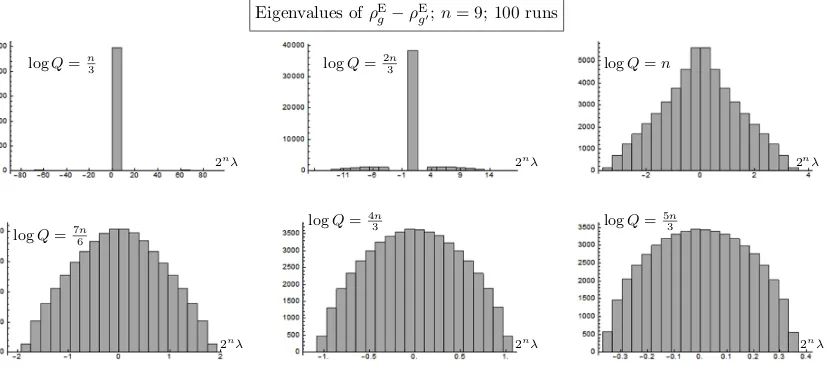
Fig. 4 shows eigenvalue histograms. We see a qualitative change asQincreases. At smallQ, there are distinct bunches of large and small eigenvalues. AtQ= 2n _{we see something resembling an} exponential or power law distribution. AtQ2n _{the distribution becomes more peaked around}

n= 9; Eigenvalues of⇢E

g(b); 100 runs

logQ=n

3 logQ=23n logQ=n

logQ=7n

6 logQ=

4n

3

logQ=5n

3

2n ₂n ₂n

2n ₂n ₂n

Figure 4: Bladiebla.

Corollary 6.4 Let2n _{nandQ 2}n_{. Let⌘ <1 be a constant. Pseudorandom-keyed 8-state}

encryption is"-randomising,"=q2n

Q(2nln 2 + 2 ln

1

⌘), except with probability⇡⌘.

Proof:In (33) we set the left-hand side to⌘and we writez="pQ/2n₌q_{2nln 2 + 2 ln}1

⌘. Using

2n _{nandQ 2}n_{we can approximate the ‘exp’ in (33) by exp(· · ·)⇡exp( z}2_{/2) = 2} n_{⌘. ⇤}

Note that the"in Corollary 6.4 becomes small for Q larger than 2n_{n·constant; this is consistent}

with theq > n+lognresult of Hayden et al [18]. Also note that Corollary 6.4 is only a probabilistic statement, with probability⌘that the statement does not hold.

Figure 4: Histogram of the eigenvalues ofρE

g(b), plotted for various values ofQ. The eigenvalues

from 100 runs are combined. The horizontal axis is scaled by a factor 2n _{so that ‘1’ corresponds}

to the eigenvalues of the fully mixed state τ.

7.6

Maximum eigenvalue of

ρ

₋

τ

Fig. 5 shows empirical data on maxi_|λi(ρE

g−τ)|=|ρEg−τ|∞. The plots are rather noisy due to the limited number of runs. We observe thatthe empirical |ρE

g −τ|∞ is orders of magnitude smaller

than the Bennett bound, for the values ofnthat we studied.

Max. absolute eigenvalue of⇢E

g(b) ⌧;n= 9; 100 runs

logQ=n

3 logQ=

2n

3 logQ=n

logQ=7n

6 logQ=

4n

3

logQ=5n

3

2n_{max| | 2}n_{max| |}

2n_{max| | 2}n_{max| |}

Figure 5: Bladiebla.

Table 3: Moments of⇢E

g(b)

t Qt_·E

btr (⇢Eg(b))t

2 Q+(Q)2

2n

3 Q+ 3(Q)2

2n +

(Q)3

22n

4 Q+ 6(Q)2

2n +

(Q)2

3n + 6

(Q)3

22n +

(Q)4

23n

5 Q+ 10(Q)2

2n + 5

(Q)2

3n + 20

(Q)3

22n + 5

(Q)3

2n₃n+ 10

(Q)4

23n +

(Q)5

24n

6 Q+ (Q)2 152n+ (

5 18)n+

15

3n2n + (Q)3 2502n+

36 3n2n+ 3(

5 36)n+

1 9n

+(Q)4 ₂503n+₃n15₂2n + 15

(Q)5

24n +

(Q)6

25n

@@ de motivatie om naar de momenten te kijken

Theorem 6.5 The moments of ⇢E

g(b) and⇢Eg(b) ⌧, averaged overb, are as given in Tables 3 and 4 respectively.

Proof:See Appendix C.

In Table 4 the contributions _{{· · · }} are negligible (at largen and Q_⌧ 3n_{) w.r.t. the preceding} terms; hence the expressions can be simplified substantially if one wants to know upper bounds only. Furthermore, forQ=_O(2n_{) the terms of orderQ/3}n_,Q/(18

5)

n_andQ2_/(36 5)

n_{are negligible}

as well.

It is interesting to look at the quantityct

def = 1

2nEbtr (⇢Eg ⌧)t. In some sense it represents the

t’th moment of the eigenvalues of⇢E

g ⌧. If one imagines that there is a probability density µ on [ 1

2n,1 ₂1n] governing the value of thei’th eigenvalue for randomi, b, g, thenct is thet’th moment ofµ. AtQ_⇡2n_{we have}

c1= 0, c2⇡( 1 2n)

2 def₌ 2_{, c}

3⇡ 3, c4⇡3 4, c5⇡6 5, c6⇡15 6. (34)

Note that c4 and c6 are exactly as in a Gaussian distribution. The odd central moments are positive because the interval [ 1

2n,1 ₂1n] extends only a little distance into the negative side.

15

Figure 5: Histogram of the maximum absolute eigenvalue of ρE

g(b)−τ, plotted for various values

of Q. The horizontal axis is scaled by a factor 2n.

7.7

Statistical properties of

ρ

₋

ρ

For completeness we also present theoretical and empirical results onρE

g −ρEg0. This is motivated by Def. 2.2.

Theorem 7.3 For any g, g0_{∈ {}0,1_}n _{with g}0_{6=g it holds that}

Ebtr ρEg(b)−ρEg0(b) 2

= 2

Q (35)

Ebtr ρE

g(b)−ρEg0(b)

3

= 0 (36)

Q3_{Ebtr ρ}E

g(b)−ρEg0(b)

4

= 2 + 8₂Qn+ 4Q

3n + 4(Q−1)

3n (−1₂)|g⊕g 0_|

− {8

2n+₃4n}. (37)

Here _|g_⊕g0_{|stands for the Hamming weight ofg⊕g}0_.

Proof: see Appendix D.

Furthermore we have_∀b :Egg0tr ρE_g(b)−ρE_g0(b) t

= 0 for oddtdue to symmetry.

Corollary 7.4 Pseudorandom-keyed QOTP encryption of classical data using the 8-state encoding is on average (w.r.t. b) statistically ε-private (Def. 2.2) withε=p2n−1_/Q.

Proof. We follow the same steps as in the proof of Theorem 6.2. Let d= 2n _{and let}

{λa}da=1 be

eigenvalues ofρE

g −ρEg0. We haveEbD(ρEg, ρEg0) = 1₂dEb1_dPa p

λ2

a ≤12d

q

1

dEbtr (ρEg −ρEg0)2. In the last step we used Jensen’s inequality. Substituting (35) givesEbD(ρEg, ρEg0)≤

q d

2Q.

Again we investigate the moments of the eigenvalues in the caseQ≈2n_{. Theorem 7.3 givess}2 def₌ 1

2nEbtr (ρE_g −ρE_g0)2 ≈( √

2

Fig. 6 shows eigenvalues ofρEg−ρEg0. As a function ofQthe same trends are visible as in Fig. 4, but now with symmetry around zero. Fig. 7 shows empirical values of|ρE

g −ρEg0|∞. Again there is a large gap between the actual numbers and the bound obtained from the matrix Bennett inequality (see below).

Eigenvalues of⇢E

g ⇢Eg0;n= 9; 100 runs

logQ=n

3 logQ=

2n

3 logQ=n

logQ=7n

6

logQ=4n

3 logQ=

5n

3

2n ₂n ₂n

2n ₂n ₂n

Figure 6: Bladiebla.

We can derive a bound similar to Theorem 6.3.

Theorem 6.8 For anyg, g0_{2 {0,1}}n _{the mixed states⇢}E

g,⇢Eg0 satisfy the following (Bennett and

Bernstein) inequalities

Prh max(⇢Eg ⇢Eg0) z

2n i

 2n_exp 

2Q

2nA( z

2) (38)

Pr

"

max(⇢Eg ⇢Eg0) z p

2

p Q2n

#

 2n_exp "

z2_/2

1 + 1 3p2z

p

2n_/Q #

. (39)

Proof:We proceed as in the proof of Theorem 6.3, but now withXj = _Q1(Pj Pj0), wherePj0= Nn

i=1| bjig0iih bjig0i|We haveEbXj= 0 and

P

jXj=⇢Eg ⇢Eg0. FurthermoreR= max(Xj) = 1/Q

and 2₌

max(PjEbXj2) = max(_Q2⌧) =_Qd2. Here we have used Theorem 6.6. Substitution into

(31) and settingt=z/din the Bennett inequality, andt=zpp_Q2₂n in the Bernstein inequality,

yields the result. ⇤.

Again we investigate the moments of the eigenvalues in the caseQ⇡2n_{. Theorem 6.6 givess}2 def₌ 1

2nEbtr (⇢Eg ⇢Eg0)2⇡(

p₂

2n)2and ₂1nEbtr (⇢Eg ⇢Eg0)4⇡10·2 4n⇡5₂s4. Note that the number 5₂ is

smaller than the ‘3’ that would hold in the case of a Gaussian distribution. Hence the distribution is narrower than Gaussian.

@ Numerics. Checken of het klopt, dmv Gaussian met zelfde variantie.

17

Figure 6: Histogram of the eigenvalues ofρE

g−ρEg0, plotted for various values ofQ. The horizontal

axis is scaled by a factor2n_.

Max. absolute eigenvalue of⇢E

g(b) ⇢Eg0(b);n= 9; 100 runs

logQ=n

3 logQ=

2n

3 logQ=n

logQ=7n

6 logQ=

4n

3

logQ=5n

3

2n_{max| | 2}n_{max| |}

2n_{max| | 2}n_{max| |}

Figure 7:Bladiebla.

7

Discussion

We briefly discuss the physical implementation of 8-state encoding. The eight photon polarisation states as depicted in Fig. 1 are not necessarily the most practical implementation. Most single-photon sources produce linearly polarised states; hence elliptic polarisation may be more difficult to handle than linear. We note that it is possible to rotate the cube in Fig. 1 in such a way that four cipherstates lie in thexz-plane [40], corresponding to linear polarisation. Another physical implementation of qubits is to use pulse trains as in Di↵erential Phase Shift QKD [38], but with di↵erent amplitudes and phases.

As topics for future work we mention (i) security proof for the proposed key recycling scheme; (ii) using the moments listed in Table 4 to derive a sharper bound on|⇢g ⌧|1and max(⇢g ⌧).

Acknowledgments

We thank Christian Scha↵ner, Serge Fehr and Andreas H¨ulsing for useful discussions.

A

Proof of Theorem 5.4

We write ⇢= | ih |. We introduce short notation Pj = Fbj| ih |Fbj†. The Pj is a projection operator satisfyingEbjPj=⌧. We have

Ebtr [⇢0(b)]t= 1 Qt

Q

X

j1=1

· · ·

Q

X

jt=1

trEbPj1· · ·Pjt. (40)

If for some a2 {1, . . . , Q}a projection Pa occurs only once in the productPj1· · ·Pjt then the

Ebreduces it to⌧. However, in thet-fold summation many di↵erent collisions can occur between the summation variables j1, j2, . . . , jt. In any of the Qt terms we denote the number ofdistinct values as k, withk2 {1, . . . , t}. There are _kt (Q)kterms with a given value ofk. At givenk, there arekdistinct projectors in the productPj1· · ·Pjt; they occur multiple times spread out over

the product. If the identical projections are direct neighbours then we can immediately use the

Figure 7: Histogram of the maximum absolute eigenvalue of ρE

g −ρEg0, plotted for various values

of Q. The horizontal axis is scaled by a factor 2n_.

Theorem 7.5 For any g, g0_{∈ {0,1}}n _{the mixed states ρ}E

g,ρEg0 satisfy

Prhλmax(ρEg −ρEg0)≥

ε

2n i

≤ 2nexp

−2₂QnA(

ε

2)

. (38)

Proof: We proceed as in the proof of Theorem 6.5, but now withXj = _Q1(Pj−Pj0), wherePj0 = Nn

i=1|ψbjig0iihψbjigi0|. We have EbXj = 0 and P

jXj =ρEg −ρgE0. Furthermore R=λmax(Xj) =

1/Q andσ2=λmax(PjEbXj2) =λmax(_Q2τ) =_Qd2 . Here we have used Theorem 7.3. Substitution

into (24) and settingt=ε/din the Bennett inequality yields the result. . From (38) we can derive an expression like Theorem 6.5 for the sufficient key length to obtain a

∞-norm version ofε-privacy; only the constant terms are different.

8

Summary and discussion

The most important results of this paper are: the introduction of the basis states|ψ000i,|ψ001ito

represent a classical bit, leading to 8-state encoding when the QOTP is applied; the key recycling scheme ‘#3’ presented in Section 4.6, which has improved noise tolerance and efficiency compared to previous proposals; bounds on the sufficient key length for pseudorandom-keyed QOTP encryp-tion of arbitrary quantum states (Theorems 6.3, 6.5 and 6.8); statistical analysis of the cipherstate eigenvalues (for classical plaintext) up to 6th order.

We briefly comment on the physical implementation of 8-state encoding. The eight photon polar-isation states as depicted in Fig. 1 are not necessarily the most practical implementation. Most single-photon sources produce linearly polarised states; hence elliptic polarisation may be more difficult to handle than linear. We note that it is possible to rotate the cube in Fig. 1 in such a way that four of the eight cipherstates lie in the xz-plane [43], corresponding to linear polarisation. Another physical implementation of qubits is to use pulse trains as in Differential Phase Shift QKD [41], but with different amplitudes and phases.

As topics for future work we mention (i) detailed security proofs for the proposed key recycling scheme; (ii) obtain sharp bounds on high moments of theρE

g eigenvalues, in order to derive tighter bounds on the sufficient key length; (iii) establish how far the actual distances|ρg−τ|1,|ρg−τ|∞ lie below the provable bounds.

Acknowledgments

We thank Christian Schaffner, Serge Fehr and Andreas H¨ulsing for useful discussions.

A

Proof of Theorem 6.6

We write ρ = _|ψ_ihψ_|. We introduce short notation Pj = Fbj|ψihψ|Fbj†. The Pj is a projection operator satisfyingEbjPj =τ. We have

Ebtr [ρ0(b)]t= 1

Qt Q X

j1=1 · · ·

Q X

jt=1

trEbPj1· · ·Pjt. (39)

If for some a ∈ {1, . . . , Q} a projectionPa occurs only once in the product Pj1· · ·Pjt then the Eb reduces it toτ. However, in thet-fold summation many different collisions can occur between the summation variablesj1, j2, . . . , jt. In any of the Qt terms we denote the number ofdistinct

values as k, with k∈ {1, . . . , t}. There are_kt (Q)k terms with a given value of k. At givenk, there arekdistinct projectors in the productPj1· · ·Pjt; they occur multiple times spread out over the product. If the identical projections are direct neighbours then we can immediately use the reduction Pm

a =Pa (m≥1). Fort≤3 there are only direct neighbours. (This follows from the circular property of the trace, trABC= trCAB). Then the expression trEbPj1· · ·Pjt reduces to trτk _{= (}1

2n)k−1, which immediately yields (26). Fort≥4, however, there are sub-expressions like

PαPβPαPβ,PαPβPγPβPαPγ, etcetera. We define an inner product on the space of 2n

×2n_{complex matrices as}

hM, N_i=EbtrM†_(b)N(b). We now use Cauchy-Schwartz, _|hM, N_i|2

≤ hM, M_ihN, N_ito bound our product expressions for

t_≥4. For example, att= 4, k= 2 we haveEbtrPαPβPαPβ =|EbtrPαPβPαPβ|=|hPβPα, PαPβi|