Hepler, Amanda Barbara. Improving Forensic Identification Using Bayesian Networks and Relatedness Estimation: Allowing for Population Substructure (Under the direc-tion of Bruce S. Weir.)
Population substructure refers to any population that does not randomly mate. In most species, this deviation from random mating is due to emergence of subpopulations. Members of these subpopulations mate within their subpopulation, leading to different genetic properties. In light of recent studies on the potential impacts of ignoring these differences, we examine how to account for population substructure in both Bayesian Networks and relatedness estimation.
Bayesian Networks are gaining popularity as a graphical tool to communicate com-plex probabilistic reasoning required in the evaluation of DNA evidence. This study extends the current use of Bayesian Networks by incorporating the potential effects of population substructure on paternity calculations. Features of HUGIN (a software package used to create Bayesian Networks) are demonstrated that have not, as yet, been explored. We consider three paternity examples; a simple case with two alleles, a simple case with multiple alleles, and a missing father case.
Networks and Relatedness Estimation: Allowing
for Population Substructure
by
Amanda B. Hepler
a dissertation submitted to the graduate faculty of north carolina state university
in partial fulfillment of the
requirements for the degree of doctor of philosophy
department of statistics
raleigh
August 15, 2005
approved by:
Dr. Bruce Weir (Chair) Dr. Jacqueline Hughes-Oliver
Amanda Hepler was born on July 26, 1977, in Frankfurt, Germany. Because her father was a career Army officer she had an opportunity to travel extensively and live in many places including Germany, Texas, Virginia, Florida, and Maryland. During her vacations with her family she visited over fifteen European countries and developed a love for traveling.
In 1995, Amanda graduated from Fallston High School, in Fallston Maryland. She attended the University of Central Florida for her first year of undergraduate stud-ies. Amanda returned to Maryland to continue her education at Towson University majoring in applied mathematics and computing. During her undergraduate program, Amanda was nominated by professors within the Mathematics Department for hon-orary membership in the Association for Women in Mathematics. She received the Mary Hudson Scarborough Honorable Mention for Excellence in Mathematics during her final year at Towson and graduated summa cum laude in 2001.
This research was supported by a graduate research grant from the National Institute of Justice. Additional funding was provided by the NCSU Department of Statistics. Office space, computing equipment, travel funding, and a superb staff were supplied by the Bioinformatics Research Center. Bruce Weir, Jacqueline Hughes-Oliver, Maria Oliver-Hoyo and Jung-Ying Tzeng all provided insightful comments, greatly improving the quality of this dissertation. Additional improvements were suggested by Ernest Hepler and Clay Barker.
Dr. Bruce Weir provided me with the tremendous opportunity of working with him during the past few years. His guidance has been invaluable and it is an honor to have been selected as one of his students. No doctoral student could have a better mentor and advisor. It has truly been a pleasure.
There have certainly been others who have influenced me during this long aca-demic journey. I began as a struggling speech pathology student at Towson University. Dr. Diana Emanuel, a hearing science professor, was the first to suggest I take a few math courses. A former psychology professor, Dr. Arthur Mueller, provided a brilliant introduction to the world of statistics. His enthusiasm and passion for the field started me on this path. Dr. Bill Swallow, a statistics professor at NCSU encouraged me to explore forensic research opportunities with Dr. Weir. These professors marked my path at critical decision points and made it possible for me to be here today.
me through this experience. David, Lisa and Laura have given me endless love and support. My three loving grandparents have never been shy in saying how proud they are of me. Their faith and encouragement are a constant source of inspiration. I would also like to thank Joel, who has been by my side and endured all the emotional “ups and downs” of this last year. He has helped me stay focused and encouraged me every step of the way. I only hope I can do half the job he’s done when it’s my turn.
List of Tables viii
List of Figures x
1 Bayesian Networks and Population Substructure 1
1.1 Introduction . . . 1
1.2 Review of Relevant Literature . . . 3
1.3 Research Methods . . . 7
1.4 Example One: A Simple Paternity Case with Two Alleles . . . 9
1.5 Example Two: A Simple Paternity Case with Multiple Alleles . . . 18
1.6 Example Three: A Complex Paternity Case with Two Alleles . . . 22
1.7 Discussion . . . 26
2 Pairwise Relatedness and Population Substructure 27 2.1 Introduction . . . 27
2.2 Review of Relevant Literature . . . 31
2.3 Research Methods . . . 44
2.4 Results . . . 55
2.5 Discussion . . . 64
3 Applications to Real Data 65 3.1 Introduction . . . 65
3.2 Pairwise Relatedness Estimation . . . 66
3.3 Multiple Allele Paternity Network Example . . . 83
3.4 Discussion . . . 85
A A Simple Bayesian Network 91
B Corrections and Comments on Wang’s Paper [1] 98
C Downhill Simplex Method C++ Code 100
C.1 C++ Function Obtaining 8D MLE . . . 100
C.2 Simplex Class C++ Header File . . . 101
C.3 Simplex Class C++ Implementation File . . . 101
C.4 Likelihood Class C++ Header File . . . 109
C.5 Likelihood Class C++ Implementation File . . . 109
1.1 Algebraic Pi Values forF ounder3 using Equation 1.6. . . 8
1.2 Numerical Pi Values forF ounder3 using Equation 1.6. . . 9
1.3 Notation for Putative Father, Mother and Child Nodes. . . 11
1.4 Paternity Index Formulas Derived in [2]. . . 17
1.5 Notation for Network in Figure 1.13. . . 23
2.1 Common θXY Values. . . 29
2.2 Similarity Index (SXY) Values for All IBS Patterns. . . 34
2.3 Conditional Probabilities Pr(λi|Sj), with No Population Substructure. . 39
2.4 Conditional Probabilities Pr(λi|Sj), with Population Substructure. . . . 42
2.5 Relationships Among Various Relateness Coefficients. . . 50
2.6 Conditional Probabilities based on Seven Parameters. . . 50
2.7 Jacquard’s Coefficients in Terms of the Inbreeding Coefficient (ψ) for Some Common Relationships. . . 53
2.8 Jacquard’s True Parameter Values for Full Siblings. . . 53
2.9 MLE, True∆Vectors, and Euclidean Distances for Example in Section 2.3. 54 2.10 Simulated Accuracy Rates for the Distance Metric Classification Methods. 62 3.1 2D, 6D and 8D MLEs, Bootstrap (BS) Standard Errors and 90% BS CIs. 68 3.2 Biases and Standard Errors for the 2D and 8D MLEs, FBI Data. . . 75
3.3 Individual Accuracy Rates for FBI Data. . . 77
3.4 Standard Errors of the 2D, 6D and 8D MLE for Selected Samples. . . . 79
3.5 Individual Accuracy Rates for HapMap Data. . . 81
3.6 CEPH Family 102 Genotypes and PI Values. . . 84
B.1 Mistaken Probabilities in Wang [1]. . . 99
1.1 Putative Father’s Node Trio. . . 10
1.2 Probability Table for Putative Father’s Paternal Gene Node. . . 10
1.3 Conditional Probability Table for Putative Father’s Genotype Node. . . 11
1.4 Network for Hypothesis, True Father and Putative Father Nodes. . . . 12
1.5 Conditional Probability Table for True Father’s Paternal Gene Node. . 12
1.6 Simple Paternity Network from Dawid et al. [3]. . . 13
1.7 Population Substructure Simple Paternity Network. . . 14
1.8 Conditional Probability Table for Mother’s Paternal Gene. . . 15
1.9 Probability Tables for Counting Nodes. . . 16
1.10 HUGIN’s Output After Entering the Evidence, Simple Paternity Network. 17 1.11 Population Substructure Paternity Network for Multiple Alleles. . . 19
1.12 HUGIN’s Output After Entering the Evidence, Multiple Allele Network. 21 1.13 Complex Paternity Network. . . 23
1.14 Population Substructure Complex Paternity Network. . . 24
1.15 HUGIN’s Output After Entering the Evidence, Complex Paternity Net-work. . . 25
2.1 Diagram of IBD Relationship Between Two Siblings X and Y. . . 28
2.2 IBD Patterns Between Two Individuals, for the Non-Inbred Case. . . . 30
2.3 IBD Patterns Between Two Individuals, for the Inbred Case. . . 42
2.4 Graph of Likelihood Function. . . 47
2.5 Graph of Likelihood Function with Intercepting Plane. . . 47
Data Points per Plot, Ten Alleles per Locus. . . 58
2.10 Standard Deviations for 2D MLE, Based on 500 Simulated Data Points per Plot. . . 59
2.11 Standard Deviations for 8D MLE, Based on 500 Simulated Data Points per Plot. . . 60
2.12 Plots of the Standard Deviations for 2D, 6D, and 8D MLEs, Based on 500 Simulated Data Points per Plot, Ten Alleles per Locus. . . 61
2.13 Accuracy Rates for 2D Method, Based on 500 Simulated Data Points per Plot. . . 63
3.1 Representative CEPH Family Pedigree. . . 66
3.2 2D, 6D and 8D MLEs for Unrelated CEPH Individuals, based on 20 or 50 loci. . . 67
3.3 P0 versus P1 Plots for Unrelated CEPH Individuals. . . 69
3.4 2D, 6D and 8D MLEs for Full Sibling and Parent Child CEPH Pairs . 70 3.5 CEPH Data Accuracy Rates for 2D, 6D and 8D Discrete Relatedness Estimates. . . 72
3.6 Plotted Biases of the 2D, 6D and 8D MLEs, FBI Data. . . 74
3.7 Plotted Standard Deviations of the 2D, 6D and 8D MLEs, FBI Data. . 74
3.8 P0 versus P1 Plots for Simulated Parent-Child Pairs from AA Sample. . 76
3.9 Mean Accuracy Rates for FBI Data. . . 77
3.10 Plotted Biases of the 2D and 8D MLEs, HapMap Data. . . 79
3.11 Mean Accuracy Rates for Hapmap Data. . . 80
3.12 P0 versus P1 Plots for Simulated Pairs from CEU Sample. . . 81
3.13 Classification Rates for the 8D Method when True Relationship is Full Sibling. . . 82
Bayesian Networks and Population
Substructure
1.1
Introduction
Population Substructure Effects on Forensic Calculations
One method of evaluating a body of evidence is to calculate a likelihood ratio [4]. This is a ratio of two probabilities:
LR = Pr(Evidence given the prosecutor’s hypothesis)
Pr(Evidence given the defendant’s hypotheses). (1.1) Generally, the defense’s hypothesis is that the evidence profile reflects someone other than the defendant. The prosecution, in contrast, argues that the match between the evidence profile and the defendant’s profile means that the defendant was the source of the evidence. The denominator of this likelihood ratio requires that a forensic scientist determine the probability of observing the same DNA profile twice, commonly referred to as the match probability [2]. The numerator is typically 1, as the prosecutor is proposing that the evidence points to the defendant. In this case, the likelihood ratio reduces to the inverse of the match probability. Likelihood ratios can take on values from 0 to ∞. If we obtain a value of 100 for our ratio, the common interpretation is “The evidence is 100 times more probable if the suspect left the evidence than if some unknown person left the evidence” [2].
possible subpopulations. People in these subpopulations could tend to mate within their subpopulation which would lead to different allelic frequencies than those esti-mated from the overall population. To estimate these possible differences, it is nec-essary to introduce a measure of background relatedness among the subpopulations under consideration. This term, typically denoted θ, is commonly referred to as the
inbreeding coefficient [4]. In 1994, Balding and Nichols proposed a method for calcu-lating match probabilities, which makes use of this inbreeding coefficient [6]. We use this methodology here, and it is further examined in Sections 1.2 and 1.3.
Bayesian Networks in Forensics
Likelihood ratios can be calculated rather simply using Bayesian Networks (also known as Probabilistic Expert Systems or Bayesian Belief Networks). A Bayesian Network (BN) is a graphical and numerical representation which enables us to reason about uncertainty. Contrary to the name, BNs are not dependent upon Bayesian reasoning. In fact, the methods and assumptions we use in this research are not Bayesian in nature, we appeal only to Bayes Theorem and probability calculus. BNs are simply a tool to make the implications of complex probability calculations clear to the layperson, without requiring an understanding of the complexity involved [7]. They provide an automated way to calculate likelihood ratios in cases where the calculations are quite laborious to perform analytically.
The use of BNs for forensic calculations has been gaining popularity over the past decade due to the development of several software packages available which make the construction of these networks relatively simple. These packages include HUGIN1
(which is used in this study), XBAIES2, Genie3, WINBUGS4, and most recently
FINEX5 [8]. A detailed discussion of BNs and their applications can be found in [9],
1
Free evaluation version available at http://www.hugin.dk
2
Free to the public, available at http://www.staff.city.ac.uk/∼rgc
3
Available at http://www2.sis.pitt.edu/∼genie
4
Free to the public, available at http://www.mrc-bsu.cam.ac.uk/bugs/winbugs/contents.shtml
5
however a brief introduction is presented in Appendix A.
In this study extensive use is made of a table generating feature of HUGIN Version 6.3. This feature allows the use of general formulas for probability tables and avoids the need to enter each probability by hand. The use of this feature should significantly reduce data entry time which historically has been one of the major complaints in using BN software.
1.2
Review of Relevant Literature
The examination of DNA evidence has become important to legal systems throughout the world. Because of this, considerable research has focused on the validity and reliability of current methods used to evaluate DNA. Two aspects of this research are reviewed. First, the current state of forensic research concerning DNA calculations, when accounting for population substructure, is summarized. It is also important to critically examine the contributions of research using Bayesian Networks to answer relevant questions in this forensic area.
Effects of Population Substructure
In 1994, Weir calculated estimates of the inbreeding coefficient, θ, using data ob-tained from the Arizona Department of Public Safety on Native American, Hispanic, African American, and Caucasian populations [11]. Weir showed a tenfold increase in θ values for the Native American sample, relative to the other samples considered. These estimates for θ ranged from 0.001 up to 0.097. Weir also demonstrated the potential impacts of using a subpopulation with a high background relatedness factor. For example, when assuming θ = 0, and an allele frequency of 0.05, the likelihood ratio obtained is 200. However, if the true value of θ was actually 0.05, the likeli-hood ratio obtained is 58. According to Evett and Weir [2], these two values could be communicated as “moderate support” (LR=58) versus “strong support.” These two interpretations could have quite a large impact when presented to a jury, and Weir’s study demonstrates that the effects of population substructure need to be taken into account when evaluating DNA evidence.
effects [of population substructure] and other sources of uncertainty” [6].
The 1996 National Research Committee (NRC) report discussed the most appro-priate way of accounting for population substructure when evaluating DNA evidence. They concluded in Recommendation 4.2 that “if the allele frequencies for the subgroup are not available, although data for the full population are, then the calculations should use the population-structure equations [derived by Balding and Nichols]” [14]. In light of this recommendation, and due to the simple nature of Balding and Nichols’ method, it is used to calculate all match probabilities in this research.
In summary, the cited research demonstrates the impact of population substruc-ture on the evaluation of DNA evidence. The chance of this background relatedness occurring in certain populations is large, and ignoring this potential could lead to er-rors in probability calculations. It seems reasonable that there is a higher amount of background relatedness among many populations, in addition to those discussed in Weir’s 1994 article. Several cultures throughout the United States have a high oc-currence of inbreeding, which speaks to the importance of ongoing research in this area. Today, DNA evidence is used routinely by courts to establish guilt or innocence. Population substructure must be considered or the credibility of this evidentiary tool could be called into question. Balding and Nichols have proposed a method of taking into account population substructure when evaluating DNA evidence. This method-ology provides a simple, effective way to incorporate population substructure into our Bayesian Network.
Bayesian Networks in Forensics
constructing legal arguments” [15, 13]. Recently, Evett et al. claimed that BNs will play an increasingly important role in forensic science and that their power lies in “en-abling the scientist to understand the fundamental issues in a case and to discuss them with colleagues and advocates [which] is something that has not been previously seen in forensic science” [16].
Researchers have examined a wide array of forensic cases over the past few years with the aid of BNs, ranging from simple car accident scenarios [17] to a highly com-plex murder case [15]. Other researchers have explored using BNs to model the most complex DNA evidence cases. The cases that have been examined to date are quite exhaustive and include: paternity determination [3, 8], taking into account muta-tion [3, 18], small quantities of DNA [16], cross-transfer evidence [19], and mixture cases with partial profiles involved [20, 21, 8].
1.3
Research Methods
Each Bayesian Network we consider here is some variation of a paternity case. In these cases, the likelihood ratio given in Equation 1.1 is termed thepaternity index, or PI. Let
E denote the evidence, P F denote putative father, M denote mother, and C denote child. Here the prosecutor’s and defendant’s hypotheses are formed by considering whether or not the putative father is the true father:
Hp: P F is the father of C.
Hd: Some other man is the father ofC.
Thus, the PI is
PI = Pr(E|Hp) Pr(E|Hd)
. (1.2)
Denote the genotype of personXasGX, and assume the only evidence is the gentoypes
of the child, mother, and putative father. Then the PI from Equation 1.2 can be rewritten as
PI = Pr(GC, GM, GP F|Hp) Pr(GC, GM, GP F|Hd)
. (1.3)
Using conditional probability properties (Box 1.2 of [2]), we have
PI = Pr(GC|GM, GP F, Hp) Pr(GC|GM, GP F, Hd)
×Pr(GM, GP F|Hp)
Pr(GM, GP F|Hd)
. (1.4)
The mother’s and putative father’s observed genotypes do not depend on which hy-pothesis is true and thus the second term is one. Therefore, the PI for the simple paternity case is the ratio of two conditional probabilities:
PI = Pr(GC|GM, GP F, Hp) Pr(GC|GM, GP F, Hd)
. (1.5)
The match probabilities needed to compute the denominator in Equation 1.5 can be calculated using the aforementioned methodology of Balding and Nichols [6]. Before we present this method, we introduce some notation (which differs from that presented in [6]). First, pi is the frequency of the ith allele in the subpopulation being studied.
of alleles observed. Finally, θ represents the inbreeding coefficient. With this notation in place, the probability of observing the ith allele, given ni alleles have already been
observed is denoted Pi, and its value can be calculated as shown in Equation 1.6:
Pi = Pr(Ai|ni) =
niθ+pi(1−θ)
1 + (n−1)θ . (1.6)
To illustrate the proper use of this formula, we give a short example. First, we refer to the kth founder allele observed as F ounderk. Suppose we have observed two alleles
in our subpopulation and would like to obtain the appropriate allele frequencies for the third allele observed, F ounder3. Also, suppose that the locus under consideration
has only two alleles, A1 and A2. The appropriate frequencies can be obtained from
Equation 1.6 and are shown in Table 1.1. For example, the formula given in the
Table 1.1: Algebraic Pi Values for F ounder3 using Equation 1.6.
F ounder1 A1 A2
F ounder2 A1 A2 A1 A2
A1 2θ+p1+θ1(1−θ) θ+p1+θ1(1−θ) θ+p1+θ1(1−θ) p11+θ(1−θ)
A2 p2(1−θ)
1+θ
θ+p2(1−θ) 1+θ
θ+p2(1−θ) 1+θ
2θ+p2(1−θ) 1+θ
first cell of Table 1.1 corresponds with Equation 1.6 by letting i = 1 (the observed value of F ounder3 is A1), n1 = 2 (two A1 alleles have already been seen), and n = 2,
(we have observed a total of two alleles). As a numerical example, we could calculate these values in the hypothetical case where θ = 0.03,p1 = 0.10, and p2 = 0.90. These
values are presented in Table 1.2. As can be seen, the allele frequencies depend upon how many of that allele have already been observed. If two A1 alleles have been seen
already, then the probability of observing another from F ounder3 increases 50% from
the original p1 value of 0.10 to 0.1524. If no A1 alleles have been observed, then the
value decreases to 0.0942.
Table 1.2: NumericalPi Values for F ounder3 using Equation 1.6.
F ounder1 A1 A2
F ounder2 A1 A2 A1 A2
A1 0.1524 0.1233 0.1233 0.0942
A2 0.8476 0.8767 0.8767 0.9058
allows us to enter formulas into HUGIN for most nodes, as opposed to having to enter each number by hand. The next section demonstrates how this method can be incorporated into a Bayesian Network.
1.4
Example One: A Simple Paternity Case with
Two Alleles
Consider the simple paternity case, where the genotypes of the mother, child and pu-tative father are known. For simplicity, we consider only one locus, with two alleles. In future networks created in this study, we incorporate evidence from multiple loci using the method endorsed by [14], which recommends that likelihood ratios be multiplied together. We also consider cases where we have several alleles at a particular locus. The BN for the simple paternity case with two alleles was first published by Dawid et al. in [3]. Here, we provide a brief description of their network, then extend it to account for population substructure.
In paternity cases, there is typically genotype data on three individuals; mother, child, and putative father. Three nodes are required in the BN to describe each in-dividual. The first two nodes represent the maternal and paternal genes (or alleles) passed down to the individual. These nodes can take on values A1 or A2, where Ai
individual represents their actual genotype. These node names will end in “gt,” for genotype, and can take on values A1A1, A1A2, or A2A2. Arrows in the network show
that the genotype node depends on the maternal and paternal gene nodes. Figure 1.1 shows the graphical representation for the putative father (pf).
Figure 1.1: Putative Father’s Node Trio.
Along with each node, there are associated probability tables. For example, the probabilitypfpgwill take on the valueA1 is the population allele frequency of the first
allele. Figure 1.2 illustrates how HUGIN represents the probability table, assuming the frequency for A1 is 0.10. The probability table will look exactly the same for the
Figure 1.2: Probability Table for Putative Father’s Paternal Gene Node.
node pfmg. For node pfgt, the probabilities are determined by the values of pfpg
and pfmg. To demonstrate, Figure 1.3 shows probability table for pfgt, conditional on pfpg and pfmg. The first cell must be one, as it represents the probability pfgt
Figure 1.3: Conditional Probability Table for Putative Father’s Genotype Node.
arguments are used to arrive at the other cell values.
As mentioned, each individual in the network will have node trios similar to that shown in Figure 1.1. The first letters of each node indicate which individual is being considered. The notation and descriptions for these nine nodes are given in Table 1.3.
Table 1.3: Notation for Putative Father, Mother and Child Nodes.
Node Description
pfpg Putative father’s paternal gene
pfmg Putative father’s maternal gene
pfgt Putative father’s genotype
mpg Mother’s paternal gene
mmg Mother’s maternal gene
mgt Mother’s genotype
cpg Child’s paternal gene
cmg Child’s maternal gene
cgt Child’s genotype
This node is termed the hypothesis node, and it will eventually be used to compute the PI given by Equation 1.5. The relationships between these three nodes, along with the putative father nodes, are shown in Figure 1.4. For all of the networks presented
Figure 1.4: Network for Hypothesis, True Father and Putative Father Nodes.
here, we make the simplistic assumption that the prior odds of putative father being the true father is one. Thus, the two entries in the probability table for node tf=pf?
are both 0.50. Conditional probabilities for nodestfpg andtfmgare similar, thus only the table fortfpgis shown in Figure1.5. If the hypothesis node is true, then the values
Figure 1.5: Conditional Probability Table for True Father’s Paternal Gene Node.
Again, the values in Figure 1.5 assume alleleA1 occurs with frequency 0.10. The entire
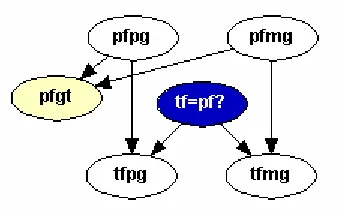
network with all twelve nodes is shown in Figure 1.6.
Figure 1.6: Simple Paternity Network from Dawid et al. [3].
To incorporate population substructure into this network we need to introduce several new nodes. First, we create a node for the value of θ and label it theta. This node takes on the value ofθwe propose is associated with our population, and can take on any value the user chooses. Next, we add a node that contains the population’s allele frequency for the A1 allele. This is denoted Specified p, and the values can
range from 0 - 1, as specified by the user. Now we need to keep track of how many
Ai alleles have already been seen. This is easily done by introducing several counting
nodes labeled n2, n3, n4, and n5. These replace the variable ni that is present in
Equation 1.6. In particular, n2 is the value of n1 after seeing two genes; n3 is the
value of n1 after seeing three genes, etc. Note that no n1 node is necessary, as we can
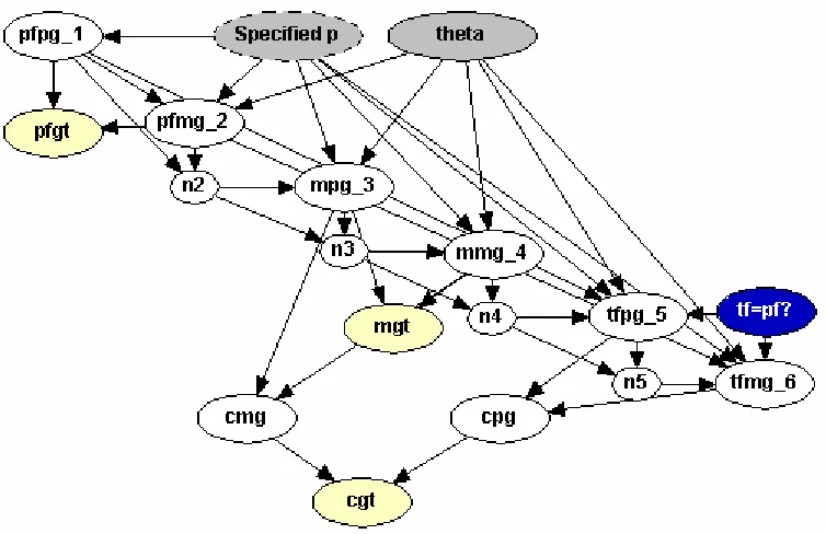
pfmg 2. The new network created appears in Figure 1.7.
Figure 1.7: Population Substructure Simple Paternity Network.
We have rearranged the nodes in this network to ensure the reader can view all relationships present among our new nodes. The relationships, represented by arrows, are simply a result of what information is needed in our formulas to generate the allele frequencies, according to Equation 1.6. Specified p and theta are needed to calculate each founder’s frequencies, therefore there are arrows from those nodes to every founder node in the graph. For the counting nodes, consider the node n3. It needs the information fromn2to know how manyAialleles have occurred up until that
point, resulting in one arrow. The node n3 also needs information from the current node to update the number of Ai occurrences, resulting in another arrow. This node
Now we must discuss the numerical portion of our network. HUGIN allows the user to specify an expression to generate a conditional probability table. There are two ways to do this: enter a distribution or enter if-then-else statements. Here, we use the distribution method. To do this, the user types the following into the Expression
line of the table: Distribution(Formula for A1, Formula for A2). In our case, the
formula for A1 is taken directly from the formula given in Equation 1.6, with n= 2 as
we have observed two founder alleles at this point, and i = 1. The formula forA2 is
simply one minus the value calculated for A1. HUGIN then generates the conditional
probability table, shown in Figure 1.8 for the node mpg 3, based on the distribution we entered.
Figure 1.8: Conditional Probability Table for Mother’s Paternal Gene.
These values can then be verified against those calculated by hand in Table 1.2, as the same values forθandp1were used. To do this, the numbers listed in Table 1.2 under
F ounder1 =A1 andF ounder2 =A1 match with the numbers listed in Figure 1.8 under
theta = 0.03,Specified p= 0.1, and n2 = 2. The numbers listed in Table 1.2 under
F ounder1 =A1 and F ounder2 =A2 as well as those listed under F ounder1 =A2 and
F ounder2 =A1 match with those listed in Figure 1.8 under theta = 0.03, Specified
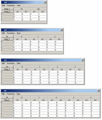
comes from simply counting how many times the A1 allele is seen.
Figure 1.9: Probability Tables for Counting Nodes.
Table 1.4, with actual PI values listed for the case when θ = 0.03 and p1 = 0.1. For
Table 1.4: Paternity Index Formulas Derived in [2].
mgt cgt pfgt P I P I (θ = 0.03, p1= 0.1)
A1A1 A1A1 A1A1 4θ+(11+3θ−θ)p1 5.02
A1A1 A1A1 A1A2 2[3θ+(11+3θ−θ)p1] 2.91
A1A1 A1A2 A2A2 2θ+(11+3θ−θ)p2 1.17
A1A1 A1A2 A1A2 2[θ+(11+3θ−θ)p2] 0.60
A1A2 A1A1 A1A1 3θ+(11+3θ−θ)p1 5.83
A1A2 A1A1 A1A2 2[2θ+(11+3θ−θ)p1] 3.47
example, consider the case when mgt = A1A1, cgt = A1A1, and pfgt = A1A2. We
would like to verify that HUGIN matches the value of 2.91 seen in Table 1.4. After entering in the evidence provided by the mother, child, and putative father, HUGIN displays the tables shown in Figure 1.10. First, note that the evidence entered is
Figure 1.10: HUGIN’s Output After Entering the Evidence, Simple Paternity Network.
“Yes” and dividing it by the value displayed next to “No,” and is given in Equation 1.7,
PI = 74.45
25.55 = 2.91. (1.7)
We attempted all of the cases presented in Table 1.4 and obtained matching results using HUGIN.
Now we would like to compare our new network with the one presented in Figure 1.6. In total, we added only six new nodes. The nodes Specified p and theta require entering in only one number each, and do not increase the complexity of the conditional probability tables associated with the other nodes. The addition of the counting nodes do, however, increase the complexity of the probability tables of other nodes. For example, the nodempg 3previously required the entry of only two probabilities. Now there are two probability entries for each value of n2, leading to a total of six entries. This type of increase occurs with each founder node. However, with the use of the table generating feature and the use of the formulas given by Balding and Nichols, no data entry for any of these nodes is required. One must simply enter the correct formula in each table and let HUGIN calculate the actual values. As a result, the amount of time needed to create our new network, after the formulas have been established, turns out to be less than that of the previous network. In addition, the two networks take an equivalent amount of time to run using a reasonably equipped personal computer. It is important to note that our new network provides the exact same results as the previous network by simply entering inθ = 0, making it flexible enough to handle both cases.
1.5
Example Two: A Simple Paternity Case with
Multiple Alleles
We arbitrarily call them Ai, i = 1,2,3,4. The allele frequencies in our population
associated with these alleles are again denoted pi. We then pool all other possible
alleles into one group, denotedX where the probability of having one of these grouped alleles would be 1−p1 −p2 −p3 −p4. Our new network needs additional nodes to
incorporate these new alleles. First, we create nodes p Ai, for i = 1,2,3,4. Each of these take on the values of the allele frequencies specified by the user. In this example, we assume that pi = 0.1 for all i. The final nodes we need to modify in this network
are the counting nodes. Previously, we recorded only how many A1 alleles were seen.
Now we must keep a count of how many A1, A2, A3, and A4 alleles are seen. We now
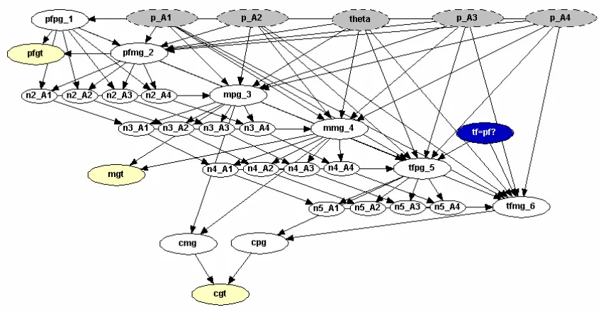
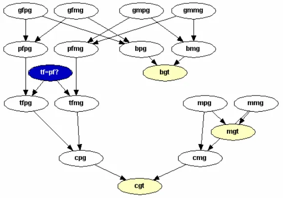
have n2 A1, n2 A2,n2 A3, andn2 A4to replacen2, andn3 A1,n3 A2, n3 A3, and n3 A4to replace n3, and so on. The new network is displayed in Figure 1.11.
Figure 1.11: Population Substructure Paternity Network for Multiple Alleles.
previously only took on the values A1 and A2. Now, it can take on values A1, A2,
A3, A4, and X. This means the entry in the Expression line has five items in the
distribution statement, instead of only two.
A more subtle difference involves the counting nodes. In this network, there is a different counting node for each of the first four alleles. There is nothing inherent in our network that requires these nodes to add up to the number of alleles we have seen. For example, consider the counting nodes for the second allele observed, n2 A1,
n2 A2, n2 A3, andn2 A4. Each of these nodes can take on values 0, 1, or 2. Thus, it is possible each node could each take on the value of two. If this situation were to occur, using Equation 1.6 with certain allele frequencies could produce negative values in some of the conditional probability table cells for the node mpg 3. To prevent this, we employ an If statement in theExpression line: If X, Distribution(A), Distribution(B). This is interpreted as “If X is true, distribution A is used. Otherwise, distribution B is used.” In this example, X represents the inequality n2 A1+n2 A2
+n2 A3+n2 A4≤2. Distribution(A) is given by Equation 1.6 andDistribution(B)
is given by the original allele frequencies. The complete statement for node mpg 3 is as follows:
if (n2_A1+n2_A2+n2_A3+n2_A4 <= 2,
Distribution ((n2_A1*theta+p_A1*(1-theta))/(1+theta), (n2_A2*theta+p_A2*(1-theta))/(1+theta),
(n2_A3*theta+p_A3*(1-theta))/(1+theta), (n2_A4*theta+p_A4*(1-theta))/(1+theta), ((2-(n2_A1+n2_A2+n2_A3+n2_A4))*theta
+ (1-(p_A1+p_A2+p_A3+p_A4))*(1-theta))/(1+theta)),
Distribution (p_A1, p_A2, p_A3, p_A4, 1-(p_A1+p_A2+p_A3+p_A4))).
For node mmg 4, the If statement will read if (n3_A1+n3_A2+n3_A3+n3_A4 <= 3, and so on. The counting node tables are created in the same manner as those in the previous example, and have not been included here due to space considerations.
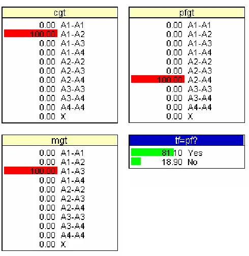
The paternity index can now be obtained from HUGIN for various cases. Here we consider the case where the mother’s genotype isA1A3, the putative father’s genotype
this case and it is shown in Equation 1.8,
PI = 1 + 3θ
2{θ+ (1−θ)p2}. (1.8)
When θ = 0.03 and p2 = 0.1, this formula gives PI = 4.29. Using HUGIN, we obtain
the same result. Figure 1.12 gives HUGIN’s output after entering in the evidence. The corresponding PI is given in Equation 1.9,
PI = 81.10
18.90 = 4.29. (1.9)
Figure 1.12: HUGIN’s Output After Entering the Evidence, Multiple Allele Network.
conditional probability tables. Each founder node would have five states instead of just two, as there are five possible alleles (A1,A2,A3, A4, or X). Each genotype node
would have a total of ten states, as there are 10 ways to select two alleles from a total of five possible alleles. Previously, each genotype had only three states (A1A1, A1A2,
and A2A2).
Our network shown in Figure 1.11 adds a total of 21 nodes to the network which does not consider population substructure. The first five (theta and p Ai, i = 1,2,3,4) only require one number entered for each node. However, the various counting nodes do add quite a bit of complexity. Typing in each of the tables associated with the counting nodes is quite time consuming, although not very complex to derive. Again, the use of the table generating feature simply nullifies any added complexity that may occur in the founder nodes due to the addition of the counting nodes. The only data entry required is the formulas for each node, which is essentially the same amount of work required in the two allele case. In terms of running time, this network takes approximately one minute to run, whereas the non-population substructure network takes approximately three seconds (again, on a reasonably equipped personal computer). This time difference is substantial, however computing time is not as much of a concern in recent times, due to increasing technology. Overall, our new network is substantially more complex than its counterpart. However, this complexity is by no means prohibitive, as it needs to be created only once. From then on, the network is flexible enough to handle any type of paternity case that could arise when all three genotypes are given (including the scenario in Example One).
1.6
Example Three: A Complex Paternity Case
with Two Alleles
a sample from a relative of the putative father. In particular, consider the case when DNA is available from a brother of the putative father. A simple network depicting this situation is provided in Figure 1.13. A table listing the new notation used in this
Figure 1.13: Complex Paternity Network.
network is shown in Table 1.5.
Table 1.5: Notation for Network in Figure 1.13.
Node Description
gmpg Mother of Putative father’s paternal gene
gmmg Mother of Putative father’s maternal gene
gfpg Father of Putative father’s paternal gene
gfmg Father of Putative father’s maternal gene
bpg Brother of Putative father’s paternal gene
bmg Brother of Putative father’s maternal gene
bgt Brother of Putative father’s genotype
network, similar to those added in the previous two examples. We add one node containing our theta value (theta), one containing our allele frequencies (Specified p), and several counting nodes (n2 - n7). For simplicity this network only considers the two allele case, however it can be extended to incorporate multiple alleles in a manor similar to Example Two. The final network, with the new nodes included, is displayed in Figure 1.14.
Figure 1.14: Population Substructure Complex Paternity Network.
index and the avuncular index was discovered in [22], and it is given by Equation 1.10.
AI = (1/2)PI + 1/2 (1.10)
Recall the PI given in Example One (Equation 1.5) where we observed genotypes from the putative father, mother and child. If instead of observing pf gt= A1A2, we
observe bpg = A1A2, according to Equation 1.10, we should obtain the AI shown in
Equation 1.11,
AI = (1/2)(2.91) + 1/2 = 1.96. (1.11) Now, we attempt to arrive at this same result using our new BN given in Figure 1.14. To arrive at the AI above, we assumed θ = 0.03 and p1 = 0.1. If we make those same
assumptions now, and we enter in our observed genotypes, HUGIN displays the results shown in Figure 1.15. We do in fact arrive at the same result given in Equation 1.11 by
Figure 1.15: HUGIN’s Output After Entering the Evidence, Complex Paternity Network.
dividing the percentages displayed in the table fortf=pf?, as is shown in Equation 1.12,
AI = 66.18
33.82 = 1.96. (1.12)
1.7
Discussion
Pairwise Relatedness and Population
Substructure
2.1
Introduction
Pairwise relatedness describes the amount of relatedness between two individuals or organisms. In our context, the amount of genetic similarity observed can be used as a measure or indicator of relatedness. To illustrate, suppose two individuals are full siblings. Their DNA will be made up of DNA passed down through their respective ancestors. Since they are siblings, they have the exact same ancestors. As a result, they will have a higher level of genetic similarity than an unrelated pair of individuals. That is, the greater the number of ancestors in common (increasing relatedness) leads to greater amounts of genetic similarity.
An important concept that helps describe genetic similarity is commonly referred to as identity by descent or IBD. Two alleles are IBD if they are direct copies of a single ancestral allele. For example, suppose X and Y are full siblings. Let X have alleles labeled aand b, and let Y have alleles labeledcandd. This particular situation is diagrammed in Figure 2.1. Here, there is a chance that a and c are IBD as they could both be a copy of the same maternal allele.
relat-Mother Father
X Y
ab cd
?
a c@@@Rb ?
d
Figure 2.1: Diagram of IBD Relationship Between Two Siblings X and Y.
edness and incorporate them into our estimation technique. However, most pairwise relatedness estimators developed thus far have ignored population substructure.
Measuring Pairwise Relatedness
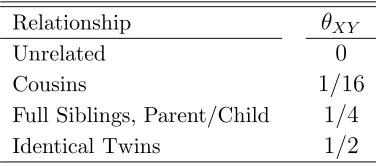
One common measure of pairwise relatedness is referred to as the coancestry coefficient, denoted θXY. It is defined as the probability a random allele from individualX is IBD
to a random allele from individual Y. To illustrate, consider the case where X and
Y are parent and child, respectively. Also assume there is no underlying population substructure (non-inbred). Suppose X has alleles a and b. Due to Mendelian inher-itance laws, with equal probability X will pass Y either allele a or allele b. Without loss of generality, we assume that a is passed from X to Y. In this case, the prob-ability of randomly selecting allele a from X is 1/2. In addition, the probability of randomly selecting allele a fromY is also 1/2. This leads to an overall probability of (1/2)(1/2) = 1/4, which is θXY in the parent-child case. Similar arguments can be
used to arrive at the other θXY values listed in Table 2.1. The relatedness coefficient
is another common measure, and is simply 2θXY (in the non-inbred case).
Table 2.1: CommonθXY Values.
Relationship θXY
Unrelated 0
Cousins 1/16
Full Siblings, Parent/Child 1/4
Identical Twins 1/2
The final and most descriptive method of measuring non-inbred pairwise relatedness was first introduced by Cotterman [29]. It involves the use of three parameters, whose definition here follows the notation of Evett and Weir [2]. Define P0, P1, and P2 as
s
s
s
s
S0
s
s
s
s
S1
s
s
s
s
S2
Figure 2.2: IBD Patterns Between Two Individuals, for the Non-Inbred Case.
In each group, the two upper dots represent the alleles in individualX. The two lower dots represent the alleles in Y. A line between two dots indicates those alleles are IBD.
patterns are required. Consider the first diagram in Figure 2.2. There are two alleles shared between X andY that are IBD. Thus, the probability of this pattern occurring is P2. The probability of the second pattern is then P1, and P0 is the probability of
the final pattern.
The coancestry coefficient can be written as a function of these “P-coefficients”. Recall θXY is the probability a random allele from individual X is IBD to a random
allele from individual Y. In the first pattern, with probability 1/2 any random allele from X will be IBD to a random allele from Y (half the time the IBD allele from Y
will be selected and half the time the non-IBD allele from Y will be selected). In the second pattern, only half of the time will you select the IBD allele fromX. When this is coupled with the chance of selecting the IBD allele from Y (1/2), you arrive at an overall probability of 1/4. The remaining pattern has no lines connecting X’s alleles toY’s alleles and therefore does not contribute to the value ofθXY. Thus the following
holds:
θXY =
1 4P1 +
1
2P2. (2.1)
potential effects of population substructure.
2.2
Review of Relevant Literature
Pairwise relatedness estimation is important in several diverse fields of study. As a result, several estimators of pairwise relatedness have been proposed using a variety of methodologies. The most commonly used technique (Queller and Goodnight [30]) was derived from a quantitative genetics point of view. The second group of estimators we consider makes use of the method of moments. Finally, maximum likelihood estimators will be reviewed. Note that the maximum likelihood approach will receive the most attention, as it is the foundation for the new estimator proposed. A comprehensive review of all techniques listed above is found in [23] and a biologist’s perspective is given in [31]. A statistical comparison of several estimators (oddly excluding maximum likelihood) is found in [32].
Queller and Goodnight’s Estimator
A commonly used technique for estimating pairwise relatedness was studied by Queller and Goodnight [30], though it was first derived by Grafen [34]. The estimate is of the relatedness coefficient (rXY) as opposed to the coancestry coefficient (θXY). They
de-rive an estimator for the average relatedness between groups of individuals, as opposed to pairs. However, they provide a modification of this method for pairwise estimation. The derivation provided in both [30, 34] is based on quantitative genetic theory. The reader is referred to [30] for details, as they are outside the scope of this review. Here, we will simply describe the estimator and discuss the advantages and disadvantages of using this technique.
First, define alleles to be identical in state (IBS) if they are of the same allelic type. It is important to note the difference between IBS and IBD. Alleles which are IBD are required to be IBS as well, because they are copies of the exact same ancestral allele. However, the reverse is not true. If two alleles are IBS, they could have descended from two different individuals (therefore not IBD). Next, label individual X’s alleles as a
and b, and individualY’s alleles as candd (these are just labels and do not necessarily imply different allelic types). Now we define indicator variables,
Sij =
1 if allele i is IBS to allele j,
0 otherwise.
(2.2)
Finally, let pi represent the population frequency of the ith allele. Queller and
Good-night’s estimate of rXY is then
ˆ
rxy =
0.5(Sac+Sad+Sbc+Sbd)−pa−pb
1 +Sab−pa−pb
. (2.3)
The value of ˆrxy will depend on which individual is assigned the label X and which is
Y. To arrive at an overall estimate, they propose using the average: ˆ
rXY + ˆrY X
Queller and Goodnight’s estimator is undefined when individualXis a heterozygote and there are only two alleles. In addition, it is possible to arrive at estimates that are outside the meaningful parameter space (0,12). According to Milligan’s [33] simulations, this estimator is unbiased, although it tends to have a left skewed distribution. Thus, the most probable estimate will often be an incorrect one. The standard error for this estimate, as with all others considered, decreases with increasing numbers of loci and alleles. A major advantage of this method is that the creators have posted a program online that is free to download and simple to use 1.
Moment Estimators
Several moment estimators have been developed to estimate pairwise relatedness [35, 36, 37, 23, 1, 38]. Two techniques are reviewed here: Li et al.’s [36] modification of Lynch’s [35] estimator; Lynch and Ritland’s [23] estimator. Of the other moment esti-mators, some are algebraically complex and others are very similar to those described below and are thus not considered in this review. Appendix B contains comments and corrections to the paper by Jinliang Wang [1].
Lynch and Li Estimator
First we consider Lynch’s [35] moment estimator, incorporating a slight modification by Li et al. [36]. They are also estimating the relatedness coefficient. To begin, define the similarity index (SXY) as the average fraction of alleles at a locus in either X or
Y for which there is another allele in the other individual which is IBS. For example, suppose X has genotype AiAi and Y has genotype AiAj. Both ofX’s alleles are IBD
to an allele from Y. Additionally, one of Y’s two alleles are IBD to an allele fromX. Thus SXY equals the average of 22 and 12 which is 34. Table 2.2 lists the SXY values
for all nine possible IBS patterns, denoted λ1, . . . , λ9. The concept behind Lynch’s
estimator is if two individuals are related to a degreerXY, the expected value ofSXY is
1
Table 2.2: Similarity Index (SXY) Values for All IBS Patterns.
IBS Patterns SXY
λ1 AiAi, AiAi ∀i 1
λ2 AiAi, AjAj ∀i,∀j6=i 0
λ3 AiAi, AiAj ∀i,∀j6=i 3/4
λ4 AiAi, AjAk ∀i,∀j6=i,∀k > j, k 6=i 0
λ5 AiAj, AiAi ∀i,∀j6=i 3/4
λ6 AjAk, AiAi ∀i,∀j6=i,∀k > j, k 6=i 0
λ7 AiAj, AiAj ∀i,∀j > i 1
λ8 AiAj, AiAk ∀i,∀j6=i,∀k6=i, j 1/2
λ9 AiAj, AkAl ∀i,∀j > i,∀k6=i, j,∀l > k, l6=i, j 0
simply the sum of two terms. The first quantity is the fraction of alleles shared because they are identical by descent and the second is the fraction shared because they are identical in state. This leads to the following equation:
E(SXY) =rXY + (1−rXY)S0, (2.5)
where S0 is the expected value of SXY at a locus for two unrelated individuals in
a randomly mating population. The value of S0 is rarely known, and Li et al. [36]
propose ˆS0 = Pni=1p2i(2−pi), where n is the number of alleles at the locus and pi is
the population frequency of the ith allele. Setting SXY equal to its expectation and
substituting in estimates for the unknown values, we have
SXY = ˆrXY + (1−rˆXY) ˆS0. (2.6)
The moment estimator is then found by solving Equation 2.6 for ˆrXY,
ˆ
rXY =
SXY −Sˆ0
1−Sˆ0
. (2.7)
To obtain a multi-locus estimate, the ˆrXY values are simply averaged over loci.
loci. . .are independent, they could be dramatically different in sampling variance and ideally should not be simply averaged to give the overall estimate” [1]. Meaningful values for rXY range from 0 to 1. It is important to note that Equation 2.7 does
require the estimates to be less than one, as SXY must be less than or equal to one.
It is possible to obtain a negative estimate, which would fall outside of the parameter space. This happens whenever SXY < S0, which occurs at times due to sampling
error [23]. Also note this estimator is always defined, as long as at least one allele frequency is greater than zero.
Lynch and Ritland’s Estimator
The next moment estimator was proposed by Lynch and Ritland [23]. To begin, define two new parameters: φXY is the probability ofX andY having one pair of IBD alleles;
∆XY is the probability of X and Y having two pairs of IBD alleles. In our notation,
these two parameters are equivalent toP1 andP2. Lynch and Ritland use these
param-eters because in quantitative genetics, they are both involved in measuring the genetic covariance between individuals. In particular, the additive genetic covariance between individuals is a function ofrXY, whereas the dominance genetic covariance is a function
of ∆XY. The relatedness coefficient can then be written in terms of these parameters:
rXY =
φXY
2 + ∆XY. (2.8)
Lynch and Ritland focus on the conditional probabilities of individualY’s genotype given individual X’s genotype. Here we will consider whenY is homozygous and refer the reader to [23] for the other possible cases. Let Pr(ii|ii) denote the probability ofX
and Y having two pairs of alleles in common and let Pr(i¯i|ii) denote the probability of them having only one pair in common. Lynch and Ritland give these probabilities as
Pr(ii|ii) =p2i +pi(1−pi)φXY + (1−p2i)∆XY, (2.9)
It is assumed that the population allele frequencies are known. To use the method of moments, two functions are required whose expected values are Pr(ii|ii) and Pr(i¯i|ii). Lynch and Ritland propose two indicator variables, that are assigned 1 if the corre-sponding genotype pattern is observed and 0 is assigned for all other patterns. These equations, with the indicator functions substituted in, can then be solved to obtain estimates for φXY and ∆XY. Using Equation 2.8, and substituting in ˆφXY and ˆ∆XY
will give the estimator:
ˆ
rXY =
ˆ
Pr(i¯i|ii) + 2 ˆPr(ii|ii)−2pi
2(1−pi)
. (2.11)
As mentioned, the equation above holds only whenY is a homozygote. Lynch and Ritland additionally provide a general form of their estimator that holds for all cases (Equation 5 in [23]). Since their estimates will differ depending on which person is labeled Y, they suggest averaging the two cases, as done by Queller and Goodnight in Equation 2.4. Finally, to obtain multi-locus estimates they propose using a weight-ing system. The actual weights that will minimize the variance of their estimator are functions of parameters and thus cannot be obtained. Lynch and Ritland use approx-imations which make the inconsistant assumption that X and Y are unrelated.
A major limitation of this estimation technique is this necessity to assume X and
Y are unrelated. It requires assuming a particular value for relatedness (namely 0), when it is relatedness itself that we are trying to estimate. As with Queller and Goodnight’s estimator above, this estimate can also be undefined. This occurs when
X is a heterozygote for a locus with two equally frequent alleles.
Another potential disadvantage is that negative estimates of rXY can occur.
Ob-taining estimates outside of the meaningful parameter space is an issue that deserves some attention. Mainly due to the competing perspectives that exist about its mean-ing. Lynch and Ritland state that these estimates are in fact meaningless, and it is a drawback to using their estimators. Milligan and Wang agree [33, 1]. However, Hardy states
‘reference population’ (or ‘reference sample’), and express a degree of ge-netic similarity between individuals relative to the average gege-netic similarity between the individuals found in the reference population. Consequently, negative values of the relatedness coefficient may be obtained, meaning X
and Y are less related on average than random individuals from the ‘refer-ence’ population.
He also states “a relatedness coefficient must always be defined relative to some refer-ence level of relatedness” [38].
Milligan [33] evaluated both moment estimators described here. Both were un-biased; however for both first cousins and unrelated individuals, almost half of the estimates fell outside the meaningful parameter space. Thus, if we were to truncate the values to lie in the meaningful space, there would be some amount of bias observed. The standard error for Lynch and Ritland’s estimator was lower than Lynch and Li’s estimator, especially in cases of low relatedness. For both estimators, standard errors are extremely dependent on the sampling conditions and on the actual degree of relat-edness. A free software program, IDENTEX, has been created by Belkhir et al. that calculates pairwise relatedness estimates using either Lynch and Ritland’s methodology or Queller and Goodnight’s technique [39].
Maximum Likelihood Estimators
As mentioned above, maximum likelihood techniques have been derived and adapted to handle a wide variety of cases. They have been used to arrive at both a discrete estimate (as done by Thompson [40]) and a continuous estimate of relatedness (as in [33]). The likelihood technique has also been extended to incorporate the effects of linkage between loci [41]. Hypothesis testing using the likelihood function has also been explored [42]. A comprehensive review of earlier work in maximum likelihood estimation and the handling of various extensions is provided in [43]. First we describe the original maximum likelihood estimator (MLE) proposed in 1975 by Thompson [40]. Then we discuss how Milligan proposed expanding Thomson’s model from three to nine parameters in order to allow for population substructure.
Three Parameter MLE
Likelihood techniques estimate the coancestry coefficient (θXY) defined in Section 2.1.
The invariance property states if ˆθ is the maximum likelihood estimator of θ, then for any function τ(θ), the MLE ofτ(θ) is τ(ˆθ). This property implies that once we obtain the MLEs for the three P-coefficients (defined in Section 2.1), we can use Equation 2.1 to find the MLE for θXY.
Assume we observe data on the genotypes of two individuals at several unlinked loci. Nine distinct IBS patterns, λi, i= 1, . . .9, were discussed in the previous section
(Table 2.2). The likelihood of P given an observed IBS pattern λi is
Li(P|λi) = Pr(λi|P). (2.12)
The subscript i on the likelihood makes it explicit that the likelihood function varies based on which IBD pattern is observed. Let the three IBD patterns in Figure 2.2 be
S7, S8, and S9 (the purpose for this notation will become clear when we discuss the
we have
Li(P|λi) = Pr(λi|S7) Pr(S7) + Pr(λi|S8) Pr(S8) + Pr(λi|S9) Pr(S9)
= Pr(λi|S7)P2+ Pr(λi|S8)P1 + Pr(λi|S9)P0.
(2.13)
If we denote the frequency of the ith allele as pi, the values for Pr(λi|Sj) are given in
Table 2.3. To illustrate, consider the first cell of Table 2.3. In this case, all alleles
Table 2.3: Conditional Probabilities Pr(λi|Sj), with No Population Substructure.
IBD Pattern IBS Pattern S7 S8 S9
λ1 AiAi, AiAi p2i p3i p4i
λ2 AiAi, AjAj 0 0 p2ip2j
λ3 AiAi, AiAj 0 p2ipj 2p3ipj
λ4 AiAi, AjAk 0 0 2p2ipjpk
λ5 AiAj, AiAi 0 p2ipj 2p3ipj
λ6 AjAk, AiAi 0 0 2p2ipjpk
λ7 AiAj, AiAj 2pipj pipj(pi+pj) 4p2ip2j
λ8 AiAj, AiAk 0 pipjpk 4p2ipjpk
λ9 AiAj, AkAl 0 0 4pipjpkpl
are of type i and we are given that two pairs of alleles are IBD. Thus, the probability of this event is the chance that X randomly gets two i alleles. When there is no population substructure, X receives the ialleles independently. Therefore it is simply the frequency of the ith allele squared. The other cells can be determined using similar arguments. This likelihood equation will be further examined and an example of its use is provided in Section 2.3.
estimates, the likelihoods for each loci are simply multiplied together to arrive at one overall likelihood function, as loci are assumed independent. This overall likelihood is then maximized to obtain the MLE. Recalling the weighting method of Lynch and Ritland that required the (perhaps incorrect) assumption thatXandY were unrelated, this multiplicative property of likelihoods is quite an advantage.
A disadvantage of the three dimensional maximum likelihood estimator is the large biases that occur for some relationships. This problem can be severe if the relationship is close to the endpoints of the parameter space. This bias occurs because the maximum likelihood technique requires its estimates to fall within the valid space. For example, if the true relationship is unrelated (θXY = 0), we will never get an unbiased result as
we are unable to obtain values less than zero. Milligan found that genetic sampling has a large effect on the amount of bias, stating that it can be reduced by sampling loci with more alleles (>20), with non-skewed frequency distributions [33]. Another disadvantage is that software is not freely available to implement this method.
An advantage of the three parameter likelihood technique is the small standard errors observed. Milligan showed, depending on sampling conditions, that the standard errors for the non-likelihood based estimators were between 2% and 250% larger. In addition he found that the errors for the MLE were less influenced by degree of actual relatedness. This was not the case for the other estimators considered. When the root mean-squared error was studied, the likelihood maintains very low values. To conclude, Milligan writes “although some non-likelihood estimators exhibit better performance with respect to specific metrics under some conditions, none approach the high level of performance exhibited by the likelihood estimator across all conditions and all metrics of performance.”
genetic data are becoming available on a much larger number of species. Thus, the likelihood method is gradually becoming a more popular method of pairwise relatedness estimation.
Nine Parameter MLE
In 2003, Milligan extended the work of Thompson by defining the maximum likelihood estimator in a way that can account for population substructure [33]. This natural extension increases the number of parameters needed from three to nine. The previous approach allowed for only three IBD patterns, as presented in Figure 2.2. When population substructure exists, there are more possibilities. There is now a chance that X’s (or Y’s) parents have ancestors in common. This implies that the two alleles received by an individual from their parent could be IBD. In particular, six additional IBD patterns must be considered. The full set of nine IBD states Sj are shown in
Figure 2.3. This expanded set of patterns requires that nine parameters be estimated:
∆j = Pr(Sj) for j = 1, . . . ,9. (2.14)
They are referred to as Jacquard’s coefficients, as they were first developed by Jacquard in [44]. The data we observe are the possible IBS patterns, λi, given in Table 2.3. Thus,
the nine parameter likelihood function is
Li(∆|λi) = 9
X
j=1
Pr(λi|Sj)∆j, (2.15)
as ∆j = Pr(Sj), and where Pr(λi|Sj) values are given in Table 2.4, adapted from [33].
We derive two cells here and refer the reader to [33] for further details.
Consider the cell in Table 2.4 corresponding to IBD pattern S4 (see Figure 2.3)
and IBS pattern λ3 (AiAi, AiAj). In this case, the two alleles from X are IBD to each
other, but no other alleles are IBD. Thus, we only need to include the probability of obtaining alleleAi once (pi). The probability ofY having alleles AiAj, given there are
s s s s @ @@ S1 s s s s S2 s s s s S3 s s s s S4 s s s s @ @@ S5 s s s s S6 s s s s S7 s s s s S8 s s s s S9
Figure 2.3: IBD Patterns Between Two Individuals, for the Inbred Case.
In each group, the two upper dots represent the alleles from individual X. The two lower dots represent the alleles fromY. A line between two dots indicates those alleles are IBD.
Table 2.4: Conditional Probabilities Pr(λi|Sj), with Population Substructure.
S1 S2 S3 S4 S5 S6 S7 S8 S9
λ1 pi p2i p2i p3i p2i p3i p2i p3i p4i
λ2 0 pipj 0 pip2j 0 p2ipj 0 0 p2ip2j
λ3 0 0 pipj 2p2ipj 0 0 0 p2ipj 2p3ipj
λ4 0 0 0 2pipjpk 0 0 0 0 2p2ipjpk
λ5 0 0 0 0 pipj 2p2ipj 0 p2ipj 2p3ipj
λ6 0 0 0 0 0 2pipjpk 0 0 2p2ipjpk
λ7 0 0 0 0 0 0 2pipj pipj(pi+pj) 4p2ip2j
λ8 0 0 0 0 0 0 0 pipjpk 4p2ipjpk
not considered within an individual; Y’s alleles could be AiAj orAjAi. Therefore, the
probability of observing IBS pattern λ3 given IBD pattern S4 is 2p2ipj. Now consider
Pr(λ7|S8). Here we observe IBS pattern AiAj, AiAj and one allele from X is IBD to
one allele from Y. One possibility is that the Ai alleles are IBD. In this case, the
probability of observing the pattern is pip2j. If, instead, the Aj alleles are IBD the
probability of observing λ7 is p2ipj. When these two probabilities are summed, we
arrive at pipj(pi+pj).
Thus, Milligan has defined a likelihood that can be maximized to find the MLEs of Jacquard’s coefficients. Making use of the MLE’s invariance property, an MLE for
θXY can be obtained. Recall θXY is the probability a random allele from individual
X is IBD to a random allele from individual Y. Using this definition, we can relate Jacquard’s parameters to θXY:
θXY = ∆1+
1
2(∆3+ ∆5+ ∆7) + 1
4∆8. (2.16)
To arrive at this equation, consider the state S1 in Figure 2.3. In this case, with
probability one, any random allele from X will be IBD to a random allele fromY. In state S3, with probability 1/2 any random allele fromXwill be IBD to a random allele
from Y (half the time the IBD allele from Y will be selected and half the time the non-IBD allele fromY will be selected). The same is true for patternsS5 andS7. InS8
only half of the time will you select the IBD allele from X. When this is coupled with the chance of selecting the IBD allele fromY (1/2), you arrive at an overall probability of 1/4. The remaining states (S2, S4, S6, and S9) have no lines connectingX’s alleles
to Y’s alleles and therefore do not contribute to the value of θXY.
2.3
Research Methods
This section extends the body of work on the estimation of relatedness using maximum likelihood techniques. First, an example of the use of the nine parameter MLE is provided. Similar to the three parameter MLE, analytical expressions for the MLE do not exist and numerical methods must be employed. The downhill simplex method is reviewed an examples of its use are provided. A new seven parameter estimator is also derived that still accounts for population substructure while reducing the number of parameters to estimate. Finally, a new methodology is developed that can infer relationships from any of the three types of MLE estimates. We conclude by describing the design of the simulation study used to compare the three, seven and nine paramter MLEs.
Nine Parameter MLE, Continued
To facilitate the understanding of the nine parameter likelihood function given by Equation 2.15, consider the following scenario. Suppose we observe genotype data for two individuals at two loci. Let individual X have alleles A1A2 at locus one and B1B2
at locus two. Let individual Y have alleles A1A1 at locus one and B1B2 at locus two.
Label the allele frequencies p1, p2 and q1, q2 at the two loci, respectively. Consider the
first locus, with IBS pattern λ5 (AiAj, AiAi). Using Equation 2.15, coupled with the
appropriate line from Table 2.4 we find the likelihood for locus one is
L5(∆|λ5) = 9
X
j=1
Pr(λ5|Sj)∆j =p1p2∆5+ 2p21p2∆6+p21p2∆8+ 2p31p2∆9. (2.17)
Now consider the second locus, and assume it is independent (unlinked) from the first locus. Here, the IBS pattern is λ7 (BiBj, BiBj). The corresponding line from
Table 2.4 leads to the likelihood
L7(∆|λ7) = 9
X
j=1
Since the loci are independent, we simply multiply the two likelihoods together to obtain an overall likelihood,
L(∆) = p1p2∆5+ 2p21p2∆6+p21p2∆8+ 2p31p2∆9
× 2q12q2∆7 +q1q2(q1 +q2)∆8+ 4q12q22∆9
. (2.19)
Now we need to maximize the likelihood, using some numerical method. Additional complexity is introduced as we have the following constraints on our parameters:
• P9
i=1∆i = 1, • 0≤∆i ≤1,∀i.
The first constraint is due to the fact that the nine IBD states are exhaustive, thus their total probability must equal one. The second constraint is simply a result of each parameter representing a probability, thus must lie between zero and one. One numerical technique that caters to functions with constraints is the downhill simplex method. For a complete description of the method, see [45]. The next section briefly describes the method and continues this example.
Downhill Simplex Method
The downhill simplex method was first described by Nelder and Mead [46]. This method was chosen because it is fast and accurate. Additional random walk methods were attempted, however the estimates obtained were exactly those of the simplex method. Additionally, the random walk programs took several hours to run, whereas the simplex method only needed seconds. The simplex method was also employed in Milligan’s study [33], allowing for verification of results.
searching for lower values. Eventually the simplex will pull itself in around the lowest point, which will be the minimum value. Throughout the process, there are constant checks to ensure the constraints are met. A C++ program was created implementing this method (see Appendix C), adapting code provided in [45]. As mentioned, this is a minimizing routine. Here we obtain the maximum value by minimizing the negative likelihood.
Recall the likelihood equation for the example provided in the previous section:
L(∆) = p1p2∆5+ 2p21p2∆6+p21p2∆8+ 2p31p2∆9
× 2q12q2∆7 +q1q2(q1 +q2)∆8+ 4q12q22∆9
.
(2.20)
We would like to maximize the likelihood with respect to ∆. For demonstration pur-poses, we consider the special case where no population substructure exists. This assumption requires ∆1 = . . .= ∆6 = 0. If we additionally assume (arbitrarily) that
p1 =p2 =q1 =q2 = 0.30, and note that ∆9 = 1−∆7−∆8, the likelihood is reduced to
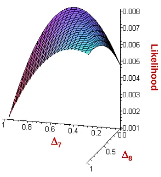
L(∆) =−0.0215∆2
7 −0.0037∆28+ 0.0168∆7+ 0.0063∆8+ 0.0047. (2.21)
Figure 2.4 provides a graph of this function.
To get a better idea of where the maximum occurs, Figure 2.5 shows the likelihood with an intercepting plane, showing the maximum occurs when ∆7 ≈0.40 and ∆8 ≈0.
We can use the simplex method to obtain exact results. The following is output from our program:
Delta 7 = 0.390 Delta 8 = 0.0 Delta 9 = 0.610 Maximum = 0.008 Theta_XY = 0.195
This method required 254 function evaluations
As predicted above, the MLEs for ∆7 and ∆8 are 0.390 and 0, respectively. The MLE
for ∆9 is simply one minus the MLE values for ∆7 and ∆8. The output gives us the