Hybrid Decision Tree using K-Means for
Classifying Continuous Data
Aparna P K
1, Dr. Rajashree Shettar
2M.Tech Student, Dept. of Computer Science, RVCE, Bangalore, India1 Professor, Dept. of Computer Science, RVCE, Bangalore, India2
ABSTRACT: One of the simplest and popular classification algorithms is the decision tree. While classification algorithms use a target attribute, Clustering algorithms group the data without a target attribute. K-Means is the simplest of the clustering algorithms. In a decision tree, branching of a nominal, ordinal, discrete or binary attribute is simple and straight forward compared to branching of a continuous attribute which is trickier, commonly creating a binary branch. Here, we present a hybrid algorithm that combines decision tree and K-Means to create multiple branches for a continuous attribute at a node. For the 9 standard datasets tested from UCI repository, the HDTKM algorithm gives an average accuracy of 78.1% and J48 gives an average accuracy of 76.1%.
KEYWORDS: Decision tree, K-Means, C4.5, Continuous data. I. INTRODUCTION
Classification deals with the prediction of an unknown attribute or target attribute from the given known attributes with the assumption that the known attributes contribute to a clear recognition of the target attribute class [1]. Decision Tree, Naïve Bayes, K-Nearest Neighbour are some of the well-known classification algorithms. The simplest of these algorithms is the Decision Tree. Many variations of the decision tree exist such as decision stump, random forest, fuzzy decision tree and so on. Some of the well-known clustering algorithms are K-Means, K-Medians, Agglomerative, Divisive, density based, grid based algorithms. Out of these K-Means is the simplest of these. Decision tree algorithm and its hybrids find lot of applications in networking [2, 3] for intrusion detection, in wireless networks [4], in medicine for detection of diseases [5,6, 7], in biometrics [8] and so on.
In this paper, a hybrid algorithm has been proposed which combines Decision Tree (C4.5) with K-Means clustering for data which contains continuous attributes.
II. RELATED WORK
Handling continuous attributes in decision tree has been subjected to its fair share of research. In [9] discussion about using hierarchical clustering algorithm to find the splits for numerical attributes during decision tree building leads to an improvement of accuracy and reduced tree size.
An effective way to handle continuous data is to discretize it. [10] uses fixed window size to divide the continuous data and discretize it. Continuous Inductive Learning Algorithm (CILA) is the new proposed discretization algorithm in [11] where the author uses class – attribute dependence to discretize the numerical data. [12] uses a discretization technique in which the maximum occurring value in each class is taken as the initial cut point. Using these initial cut points, entropy- MDLP calculations are used to arrive at final cut points. In [13], authors have used a multi interval discretization of numerical attributes. In [14] use of variance for finding the best attribute for split at each node has been proposed. In [15], the authors use the concept of mutual information to avoid selecting a previously selected attribute (happens for continuous attributes) while building the decision tree. In [16], a modification in the gain calculation of the attributes has been proposed. The authors suggest that since for a numerical attribute with many distinct values, the choice of selecting the split point is also many (which is not true for discrete attributes). This causes a bias which needs to be adjusted. The use of a node split measure called Modified Gini Index (MGI) for splitting numbered attributes is used in [17].
There are other hybrid algorithms that combine K-Means and Decision tree.
in determining the acceptability of interactive cable television in a region in [21], for breast cancer diagnosis in [6]. The authors of [22] propose a Layered Decision Tree (LDT) where each cluster from the K Means clustering becomes a layer of the decision tree. In [23], at each node of the hybrid decision tree, the data is split as per decision tree analysis and information gain is calculated. For the same data, cluster analysis is done at the node and information gain is calculated. The higher information gain of the two – decision tree and clustering is selected as the methodology for splitting at that node.
An SVM based decision tree that uses kernel KMeans clustering is proposed in [24] where each pair of leaf nodes is a SVM classifier. The combination of Association Rule Mining and C4.5 decision tree is used to classify images for brain tumour in [25] by building an FP tree from the pre-processed images.
III.BACKGROUND
A) Decision Tree:
A decision tree is a top-down; root to leaves structure where every node is either a leaf node or a single attribute that is branched further. To decide the attribute that is to be branched, in C4.5, the gain ratio of all attributes is calculated [3] as given in equation (1).
Gain ratio(A) = Gain (A)
SplitInfo (A) (1)
where A is the attribute being considered. The Gain(A) is given by equation (2).
Gain(A)=Info(D)-InfoA(D) (2)
Here, D is the subset of records at the branch of the decision tree. Further expanding, Info(D) and InfoA(D) are
given by equations (3) and (4)
Info(D) = − mi=1pilog2(pi) (3)
Where pi is the probability that an arbitrary record in D belongs to class Ci and is given by Ci,D / D
And
InfoA(D) =
Dj
D ∗ info(Dj)
v
i=1 (4)
Where Dj contains records that have value ajfor attribute A and v is the number of distinct values for attribute A.
Split info is given in equation (5).
Split InfoA D =-
Dj
D v
j=1 ∗ log2(
Dj
D ) (5)
The attribute with the maximum gain ratio is selected for branching. The branches have a subset of records from the parent branch. The subsets are decided based on the splitting algorithm. For discrete attributes, the splitting algorithm simply separates the unique values for that attribute. But for continuous data, this task is not simple. The traditional approach is to find a midpoint value and create two subsets. One subset contains records that are greater than or equal to the midpoint value and the other subset contains records that are lesser than the midpoint value. For a discrete attribute, after a branch is grown, that attribute is not considered for further gain ratio calculations. This is true for discrete attributes. The same cannot be done for continuous attributes. The tree is built till the termination condition is met, either all the records have the same value for target class or there are no attributes left for calculating the gain ratio. For continuous attributes, the attribute is not removed from the list and is used for further calculations. So, the tree continues to grow till all the records have exhausted.
The algorithm for C4.5 [27] is given below.
Algorithm : Build C4.5 Decision Tree
Input : The training data T, the attributes_available for computing the next branch
Output: A C4.5 decision tree
Method:
(1) create a node N.
(3) return N as a leaf node with target class. (4) if attributes_available is empty
(5) return N as leaf node with maximum target class for the records. (6) Get best_attribute (T, attributes_available).
(7) If best_attribute is discrete valued
(8) attributes_available = attributes_available – best_attribute. (9) Split the records based on best_attribute(best_attribute, T)
//for each split, grown a subtree by calling the //Build C4.5 Decision Tree function (10) for each split Ti of T on best_attribute
attach a new node returned by buildC4.5DecisionTree(split records Ti, attributes_available)
(11) end for (12)end function
The best attribute is calculated based on the gain ratio for the attributes as given in equations (1) – (5). If the attribute is discrete valued, then each discrete value of the attribute is grown as a branch as given in figure 1. In fig 1, the attribute animals is split into 5 branches cat, dog, sheet, rat and pig and the records are split at the node „Animals‟ based on their values for the attribute. The records that have value „Cat‟ for attribute „Animals‟ belong to the first branch and so on.
Fig 1 Split for discrete attribute
If the best attribute is continuous valued attribute, then a binary branch is grown as given in figure 2. The split for continuous attribute is usually taken as the midpoint of the values of the attribute. In fig 2, assuming that the arribute „age‟ has values from whose midpoint is 30, all the records that have value of age less than or equal to 30 belong to the left branch and all the remaining records belong to the right branch.
Fig 2 Binary split for continuous attribute.
B) K-Means:
the cluster it is closest to (minimum distance). The cluster centroids are recalculated after assignment of records. Each record is again checked if the cluster it is assigned to is correct by calculating its distance from each cluster and assigning it to the nearest cluster. These iterations continue till there are no more changes in the record assignments to the clusters. The clusters containing the records vary as the centroids vary based on record assignments.
The algorithm for K Means algorithm is given below.
Algorithm: K-Means Clustering [26]
Input: K- the number of clusters and R the records of the dataset.
Ouptut: K clusters
Method:
(1) Randomly choose K objects and make them the K cluster centroids (2) Do
(3) For each record in R
(4) Calculate distance between each cluster centroid and the record. (5) Assign the record to the cluster that has the minimum distance.
(6) Recalculate the cluster means (the values of attributes in the cluster / number of records in the cluster). (7) End for loop
(8) While records assignment to clusters do not change (9) End function
Euclidean distances are calculated from plain data which are not standardized [27]. IV.PROPOSED ALGORITHM
The problem with handling continuous attributes using binary branches is that the resultant tree is very large and requires pruning. One cannot be sure that the binary split gives the best result for continuous attributes.
The proposed algorithm performs K-Means clustering to split the continuous attribute into K branches. The K value for clustering is decided by the cut points. Cutpoints are found by first sorting the continuous attribute values in ascending order and finding the boundaries of continuous attribute values with respect to target class variations. This, most of the time, leads to a very large number of cutpoints (over 100) which is not very practical. Hence, a control factor called MINIMUM_RECORDS_PER_CLUSTER is introduced. During the K-Means algorithm iterations, any cluster that doesn‟t contain minimum records is deleted and the records of that cluster are reassigned to other clusters. This ensures that the end result is a limited number of clusters (branches). One more control parameter is WEIGHT_OF_ATTRIBUTE. During K Means clustering, the distance measure used is Weighted Euclidean distance where the continuous attribute at the node for which split is calculated will have the weight specified by the user and the rest of the attributes have unit weight.
The two control parameters, MINIMUM_RECORDS_PER_CLUSTER and WEIGHT_OF_ATTRIBUTE affect the accuracy of the classification. The proposed algorithm is given below. The tree construction is same as C4.5 except the way splits are done for continuous attribute. The splits are done using K Means clustering which is given in algorithm below.
Algorithm : Build HDTKM Decision Tree
Input : The training data T, the attributes_available for computing the next branch
Output: A HDTKM decision tree
Method:
(1) create a node N.
(2) if all records in T have same target class (3) return N as a leaf node with target class. (4) if attributes_available is empty
(5) return N as leaf node with maximum target class for the records. (6) Get best_attribute (T, attributes_available).
//for each split, grown a subtree by calling the //Build HDTKM Decision Tree function (9) for each split Ti of T on best_attribute
attach a new node returned by build HDTKM DecisionTree(split records Ti, attributes_available)
(11) end for (12)end function
For discrete attributes, the split function basically divides the records into distinct values of the attribute and each branch from the node of that attribute has a unique value and its records.
For a continuous attribute, however, K Means clustering is performed. The algorithm for the same is given below.
Algorithm: K Means clustering for HDTKM
Input: continuous attribute „C‟ being considered for split, list of cutpoints, records
Output: Group of clusters where each cluster has minimum records and each cluster is a branch from the node for the attribute „C‟
Method:
(1) create clusters same as number of cutPoints with initial cluster centroid as the cutPoint (2) do
(3) for each record in records
(4) calculate the nearest cluster for each record
(5) if nearest cluster for the record is different from previous cluster assignment for the record (6) flag change in record assignment values
(7) re/assign record to nearest cluster
Note: Nearest is based on Weighted Euclidean distance between the record attributes and cluster centroid (8) calculate the cluster centroid (average)
(9) end loop
(10) if no change in record assignment values (11) for each cluster
(12) if number of records in cluster is less than minimum_records_per_cluster (13) remove records from the cluster.
(14) Reassign these records to existing clusters (15) delete that cluster
(16) flag change in record assignment values (17) while no change in record assignment values (18) end loop
(19)end function
The weighted Euclidean distance formula is given in equation (6). Let the record attributes be a1, a2,…., an and the
cluster centroid for the same attributes be c1, c2,…., cn. The weights given by w1, w2,…., wn is equal to the
WEIGHT_OF_ATTRIBUTE (W) for the selected_attribute and it is 1.0 for every other attribute value.
Weighted Euclidean Distance = w1(a1− c1)2+ w2( a2− c2)2+ ⋯ + wn(an− cn)2 (6)
V. EXPERIMENTAL RESULTS
The HDTKM algorithm was tested against J48 algorithm from WEKA for nine different standard datasets from the UCI repository. J48 is WEKA‟s java implemention of C4.5 algorithm. The datasets chosen have continuous attributes primarily or they have discrete attributes expressed in numbers. The detail of the datasets used is given in Table 1.
Table 1 Dataset Details
Datasets Dataset size No of attributes
Balance-scale 625 5 Breast cancer 683 10 Diabetes 768 9 Ecoli 336 8 Glass 214 10 Iris 150 5 Liver disorder 345 7 Seeds 210 8 Yeast 1484 9
The first column in Table 1 is the dataset name, the second column mentions the number of records for the dataset that are used for experimentation and the last column is the number of attributes in the dataset including the target attribute. Yeast dataset contains the maximum number of records and Iris dataset contains the least. Glass dataset contains the highest number of attributes (10), Balance-scale and Iris datasets contain the least number of attributes (5).
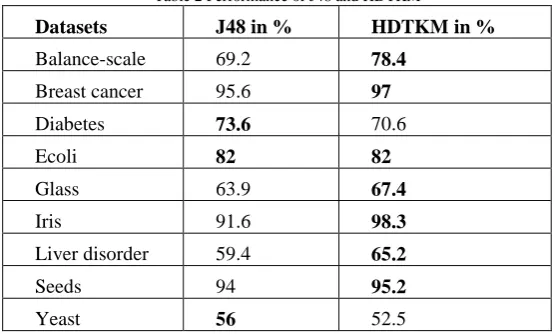
The table showing the classification accuracy for various datasets for J48 and HDTKM is given in Table 2. The higher of the two accuracies between J48 and HDTK is highlighted in bold. Balance-scale dataset is classified better by HDTKM with an accuracy of 78.4%. Breast cancer dataset is better classified by HDTKM with an accuracy of 97%. J48 classifies Diabetes dataset with higher accuracy of 73.6%. Ecoli dataset is classified with the same accuracy of 82% by J48 and HDTKM algorithms. HDTKM algorithm classifies Glass, Iris, Liver Disorder and Seeds dataset with higher accuracy than J48 with the accuracy being 67.4%, 98.3%, 65.2% and 95.2% respectively. Yeast dataset classification is higher for J48 with an accuracy of 56%.
Table 2 Performance of J48 and HDTKM
Datasets J48 in % HDTKM in %
Balance-scale 69.2 78.4
Breast cancer 95.6 97
Diabetes 73.6 70.6 Ecoli 82 82
Glass 63.9 67.4
Iris 91.6 98.3
Liver disorder 59.4 65.2
Seeds 94 95.2
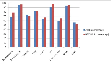
The column chart corresponding to the table for accuracy is given in Fig 3. From the graph it is clear that the HDTKM algorithm shows improvement in accuracy over J48 in 6 out of 9 datasets tested and the accuracy of J48 and HDTKM is same for Ecoli dataset.
Fig 3 Classification Accuracy of J48 and HDTKM
The datasets balance-scale, breast cancer, glass, iris, liver disorder and seeds are classified better by HDTKM algorithm. The Diabetes and Yeast datasets are classified better by J48 algorithm while the dataset Ecoli has the same classification accuracy for both J48 and HDTKM algorithm. The average classification accuracy of HDTKM is 78.1% and 76.1% for J48 algorithms.
VI.CONCLUSION AND FUTURE WORK
HDTKM algorithm performs better than J48 algorithm for the 9 standard datasets tested so far. HDTKM algorithm is suitable for classifying datasets that contain continuous attributes.
There are various options for expansion of HDTKM including using other clustering techniques such as DBSCAN, agglomerative clustering and so on. HDTKM algorithm can be optimized for all types of attributes and in any format.
REFERENCES
1. Yuhua Qian, Member, IEEE, Hang Xu, Jiye Liang, Bing Liu, and Jieting Wang. “Fusing monotonic decision trees”. IEEE, pp 1- 13, 2015.
2. Amuthan Prabakar, Muniyandi, R. Rajeswari and R. Rajaram. “Network Anomaly Detection by Cascading K-Means Clustering and C4.5 Decision Tree algorithm”. Procedia Engineering, vol. 30, pp 174 – 182, 2012.
3. Neha G. Relan and Prof. Dharmaraj R. Patil. “Implementation of Network Intrusion Detection System using Variant of Decision Tree Algorithm”.International Conference on Nascent Technologies in the Engineering Field IEEE, pp 1 - 5, 2015.
4. Khalid K. Almuzaini and T. Aaron Gulliver. “Localization in Wireless Networks using Decision Trees and K-means Clustering”. IEEE, pp 1 – 5, 2012.
5. Hind Elouedi, Walid Meliani, Zied Elouedi and Nahla Ben Amor. “A Hybrid Approach Based on Decision Trees and Clustering for Breast Cancer Classification”. IEEE, 2014, pp 226 – 231.
6. YOOHYEON CHO, YEAHJI AHN, SUBIN YOON, JINWON KWON, and TAESEON YOON. “Analysis of Anti-cancer Cytokines by Apriori Algorithm, Decision Tree, and SVM”. IEEE, pp 232 – 237, 2015.
7. Dipen Somani and Shanmuganathan Raman. “Decision Tree for Corner Detection”. IEEE, pp 1 - 5, 2015. 0
10 20 30 40 50 60 70 80 90 100
J48 (in percentage)
8. V. V. Satyanarayana Tallapragada and Dr. E. G. Rajan. “Morphology Based Non Ideal Iris Recognition using Decision Tree Classifier”. International Conference on Pervasive Computing, IEEE, pp 1 – 4, 2015.
9. Fernando Berzal, Juan-Carlos Cubero, Nicolas Marın and Daniel Sanchez. “Building multi-way decision trees with numerical attributes”. Information Sciences, vol. 165, pp 73 – 90, 2004.
10. Yiqun Zhang and Yiu-ming Cheung. “Discretizing Numerical Attributes in Decision Tree for Big Data Analysis”. IEEE, vol. 103, pp 1150 – 1156, 2014.
11. Ali Al-Ibrahim. “Discretization of Continuous Attributes in Supervised Learning algorithms”. The Research Bulletin of Jordan ACM, vol. 2 (4), 2011, pp 158 – 166, 2011.
12. B.Hemada and K.S.Vijaya Lakshmi. “Discretization Technique Using Maximum Frequent Values and Entropy Criterion”. International Journal of Advanced Research in Computer Science and Software Engineering, vol. 3 (11), pp 231 – 237, 2013.
13. YAN-HUANG JIANG, HAI-FANG ZHOU and XUE-JUN YANG. “CONSTRUCTING DECISION TREE WITH CONTINUOUS ATTRIBUTES FOR BINARY CLASSIFICATION”. IEEE, pp 617 – 622, 2002.
14. Ramesh Konda and K. P. Rajurkar. “A Rule Induction Algorithm for Continuous Data Using Analysis of Variance”. IEEE, pp 489 – 494, 2005.
15. HUA LI, XI-ZHAO WANG and YONG LI. “USING MUTUAL INFORMATION FOR SELECTING CONTINUOUS-VALUED ATTRIBUTE IN DECISION TREE LEARNING”. IEEE, pp 1496 – 1499, 2003.
16. J R Quinlan. “Improved Use of Continuous Attributes in C4.5”. Journal of Artificial Intelligence Research, vol. 4, pp 77 – 90, 1996. 17. Anuradha and Gupta, G.. “MGI: A New Heuristic for classifying continuous attributes in decision trees”. IEEE, pp 291 – 295, 2014. 18. Md. Hedayetul Islam Shovon and Mahfuza Haque. “An Approach of Improving Student‟s Academic Performance by using K-means
clustering algorithm and Decision tree”. International Journal of Advanced Computer Science and Applications, vol. 3 (8), pp 146 – 149, 2012.
19. Yi-Hui Liang. “Combining the K-means and decision tree methods to Promote Customer Value for the Automotive Maintenance Industry”. IEEE, pp 1337 – 1341, 2009.
20. Yang Huaizhen and Li Lei. “Order Prediction of Interactive Service of Cable Television Based on K-means Cluster and Decision Tree”. International Conference on Computer Application and System Modeling, IEEE, pp 215 – 219, 2010.
21. Nura Esfandiary and Amir-Masoud Eftekhari Moghadam. “LDT: Layered Decision Tree based on Data Clustering”. 13th Iranian Conference on Fuzzy Systems, IEEE, pp 1 – 4, 2013.
22. Masaki KUREMATSU and Hamido FUJITA. “A Framework for Integrating a Decision Tree Learning Algorithm and Cluster Analysis”. 12th IEEE International Conference on Intelligent Software Methodologies, Tools and Techniques, pp 225 – 228, 2013.
23. Jianhua Zhang. “Decision Tree SVM Basing on Kernel Clustering”. IEEE, pp 5791 – 5794, 2011.
24. P. Rajendran and M.Madheswaran. “Hybrid Medical Image Classification Using Association Rule Mining with Decision Tree Algorithm”. JOURNAL OF COMPUTING, vol. 2 (1), pp 127 – 136, 2010.
25. Daniel Berry, Jason Bell and Edward Sazonov. “Detection of Cigarette Smoke Inhalations from Respiratory Signals Using Decision Tree Ensembles”. Proceedings of the IEEE SoutheastCon, pp 1 – 4, 2015.
26. Dibya Jyoti Bora and Dr. Anil Kumar Gupta. “Effect of Different Distance Measures on the Performance of K-Means Algorithm: An Experimental Study in Matlab”. International Journal of Computer Science and Information Technologies, vol. 5 (2), pp 2501 – 2506, 2014.
27. Gaurav L Agrawal and Hitesh Gupta. “Optimization of C4.5 Decision Tree Algorithm for Data Mining Application”. International Journal of Emerging Technology and Advanced Engineering, vol 3 (3), pp 341 – 345, 2013.
BIOGRAPHY
Aparna P K is a student pursuing her MTech in Computer Science from RV College of Engineering, Bangalore, India. She has 4 years of industry experience. Her research interests are Data Mining, Decision Trees etc.