University of Windsor
University of Windsor
Scholarship at UWindsor
Scholarship at UWindsor
Electronic Theses and Dissertations
Theses, Dissertations, and Major Papers
2009
A Distributed Algorithm for Finding Separation Pairs in a
A Distributed Algorithm for Finding Separation Pairs in a
Computer Network
Computer Network
Katayoon Moazzami
University of WindsorFollow this and additional works at: https://scholar.uwindsor.ca/etd
Recommended Citation
Recommended Citation
Moazzami, Katayoon, "A Distributed Algorithm for Finding Separation Pairs in a Computer Network" (2009). Electronic Theses and Dissertations. 330.
https://scholar.uwindsor.ca/etd/330
This online database contains the full-text of PhD dissertations and Masters’ theses of University of Windsor students from 1954 forward. These documents are made available for personal study and research purposes only, in accordance with the Canadian Copyright Act and the Creative Commons license—CC BY-NC-ND (Attribution, Non-Commercial, No Derivative Works). Under this license, works must always be attributed to the copyright holder (original author), cannot be used for any commercial purposes, and may not be altered. Any other use would require the permission of the copyright holder. Students may inquire about withdrawing their dissertation and/or thesis from this database. For additional inquiries, please contact the repository administrator via email
A DISTRIBUTED ALGORITHM FOR FINDING SEPARATION PAIRS IN A
COMPUTER NETWORK
by
KATAYOON MOAZZAMI
A Thesis
Submitted to the Faculty of Graduate Studies
through Computer Science
in Partial Fulfillment of the Requirements for
the Degree of Master of Science at the
University of Windsor
Windsor, Ontario, Canada
2009
Author’s Declaration of Originality
I hereby certify that I am the sole author of this thesis and that no part of this thesis has been
published or submitted for publication.
I certify that, to the best of my knowledge, my thesis does not infringe upon anyone’s copyright nor
violate any proprietary rights and that any ideas, techniques, quotations, or any other material from
the work of other people included in my thesis, published or otherwise, are fully acknowledged in
accordance with the standard referencing practices. Furthermore, to the extent that I have included
copyrighted material that surpasses the bounds of fair dealing within the meaning of the Canada
Copyright Act, I certify that I have obtained a written permission from the copyright owner(s) to
include such material(s) in my thesis and have included copies of such copyright clearances to my
appendix.
I declare that this is a true copy of my thesis, including any final revisions, as approved by my thesis
committee and the Graduate Studies office, and that this thesis has not been submitted for a higher degree to any other University or Institution.
Abstract
One of the main problems in graph theory is the question of graph connectivity. Graph connectivity
often arises in problems related to network reliability. Graph connectivity can be studied from
two different aspects, namely, vertex-connectivity and edge-connectivity. Vertex connectivity is the smallest number of vertices whose deletion will cause a connected graph to be disconnected. The
focus of this work is on finding separation pairs of a graph which is the set of pairs of vertices
that deleting them would disconnect a graph. Finding separation pairs can be used in solving
the problem of vertex-connectivity and finding the triconnected components of the graph. There
have been different algorithms presented during the past which are non-linear or if linear, very complicated. This work is based on the work of Tarjan and Hopcroft which finds the separation
pairs in linear time, that is achieved by the use of Depth-First Search (DFS). Our goal is to present an
algorithm that finds the separation pairs in an asynchronous distributed computer network using
distributed Depth-First search (DDFS).
Dedication
I would like to dedicate this thesis to my wonderful parents and kind friends.
Acknowledgements
I am very grateful to my supervisor, Dr. Y.H. Tsin for his valuable guidance during my thesis work
and through completion of my degree requirements. Without his support, this thesis could not
have been completed. I also would like to thank members of my master committee, Dr. Z. Kobti,
Dr. G. Lan for their helpful advice and guidance.
I acknowledge the financial support from my supervisor, Dr. Y.H. Tsin, in the form of research
assistantship through NSERC; from the School of Computer Science, in the form of graduate
assistantship.
Contents
Author’s Declaration of Originality iii
Abstract iv
Dedication v
Acknowledgements vi
List of Figures ix
List of Tables x
1 Introduction 1
1.1 Introduction . . . 1
1.1.1 Motivation . . . 3
1.1.2 Previous related works . . . 4
1.1.3 Contribution of this thesis . . . 5
1.2 Organization of this thesis . . . 5
2 Definitions 6 2.1 Basic Definitions . . . 6
2.2 Depth-first Search . . . 10
2.2.1 Some Definitions Related To DFS . . . 12
3 Sequential Algorithm 13 3.1 The Sequential Algorithm Of Hopcroft And Tarjan . . . 13
CONTENTS viii
3.2 A Characterization of Separation Pairs . . . 14
3.3 A High-level Description of the Algorithm . . . 15
4 The Distributed Model 19 5 The Distributed Algoithm 22 5.1 The Distributed Algorithm . . . 22
5.1.1 Determininglowpt1,lowpt2 andnd(v) . . . 24
5.1.2 Constructing the acceptable adjacency structure . . . 28
5.1.3 Recalculatingdfs(v),lowpt1(v),lowpt2(v) . . . 30
5.1.4 Determining the Separation Pairs . . . 32
6 Conclusion 43
Bibliography 45
List of Figures
2.1 Directed and undirected graphs . . . 7
2.2 A graph and its adjacency list . . . 10
2.3 DFS traversal . . . 11
3.1 Separation pairs[20] . . . 15
List of Tables
4.1 Different DDFS algorithms and their complexities[47] . . . 20
Chapter 1
Introduction
1.1
Introduction
Graph connectivity has always been one of the most important problems explored in graph
the-ory. Some of the most common uses of graph connectivity are in communication networks like
telephone networks where the reliability of the network can be determined. Other applications
are in irreducibility analysis of Feynman diagrams in quantum physics and chemistry, scheduling
problem in operational research and circuit-layout problems.
A graph isk-vertex-connected(k-edge-connected, respectively) if removing less thankvertices (edges,
respectively) will not result in a disconnected graph. Clearly, we are interested in the cases where
k≥2. A 2-vertex-connectedgraph is commonly called abiconnectedgraph while a 2-edge-connected
graph is commonly called abridge-connectedgraph. A 3-vertex-connectedgraph is also called a
tri-connectedgraph.
Despite the fact that a tremendous amount of effort had been put into the studies of the graph connectivity problems, efficient algorithms are known only fork≤4.
Fork=2, the first biconnectivity algorithm was presented by Tarjan[42] The algorithm runs on the RAM (the standard sequential computer model) and takesO(|V|+|E|) time and space for a
con-nected graphG=(V,E). The algorithm also solves the brige-connectivity problem. Later, Hopcroft and Tarjan presented an optimal algorithm for triconnectivity[20]. Both algorithms are based on a
CHAPTER 1. INTRODUCTION 2
graph traversal technique calleddepth-first search. Later, Gabow revisited depth-first search from a
different perspective - the path-based view - and presented new depth-first-search-based optimal algorithm for biconnectivity and bridge-connectivity[16]. Galil and Italiano[17] presented the first
3-edge-connectivity algorithm. Their method is to use reduction to transform the 3-3-edge-connectivity
problem to the 3-vertex-connectivity problem and then use the triconnectivity algorithm of Hopcroft
el al. to solve the problem. The algorithm runs in optimal time and space. Owing to the fact that the
algorithm of Galil et al. is rather complicated, a few simpler optimal algorithms were then reported
by Taoka et al.[41], Nagamochi and Ibaraki[35] and Tsin[44],[48].
Efficient algorithms for other computer models have also been proposed. For the PRAM (the paral-lel RAM) model, for the biconnectivity problem, Tsin and Chin [49] presented an algorithm that runs
on the CREW (concurrent-read-exclusive-write) PRAM. The algorithm takesO(log2(|V|)) time using
O(|V|2/log2(|V|)) processors (Note: log denotes log
2) which is optimal for dense graphs. Tarjan and
Vishkin[43] developed an algorithm for the CRCW (concurrent-read-concurrent-write) PRAM that
takesO(log(|V|)) time usingO(|V|+|E|) processors. For triconnectivity, a number of algorithms had
been reported[37, 33,14] and all are very complicated. Each of them gives rise to a complicated
non-optimal sequential algorithm. For 4-vertex-connectivity, Kanevsky and Ramachandran presented
an algorithm for finding all the separating triples (sets ofthreevertices whose removal results in a
disconnected graph)[22]. The algorithm runs on theArbitraryCRCW PRAM inO(log2n) time using
O(n2) processors. It also gives rise to a sequential algorithm that runs inO(n2) time and space.
On the External-Memory model, Chiang et.al. presented the first I/O-efficient biconnected compo-nent algorithm[10]. The algorithm is an adaption of the biconnected compocompo-nent PRAM algorithm
of Tarjan et.al[49] based on simulation. It performsO(min{sort(V2),log(V/M)sort(E)}) I/Os. Using
an External-Memory connected component algorithm of Munagala et al[34], Meyer showed that
the I/O bound of the biconnected-component algorithm of Chiang et. al. can be improved to
O((E/V)sort(V)·max{1,log log(|V|DB/|E|)}). Note that (|E|/|V| ·sort(|V|))= Θ(sort(|E|)).
On the distributed computer model, a number of algorithms that run inO(|V|) time and transmits
O(|E|) messages ofO(log|V|) length had been proposed[4,12,29,39]. In the fault-tolerance setting,
with the assumption that a breadth-first search or depth-first search spanning tree is available,
CHAPTER 1. INTRODUCTION 3
rounds (dis the diameter of the graph) using O(|V|4log4) bits per processor; Devismes [13]
im-proved the bounds toO(H) moves (His the height of the spanning tree) andO(|V|log4) bits per
processor, and Tsin[44] further improved the result toO(dnlog4) rounds andO(|V|log4) bits per
processorwithout assuming the existence of any spanning tree.For 3-edge-connectivity, Saifullah
and Tsin[46] presented a self-stabilizing algorithm that can identify all the 3-edge-connected
com-ponents inO(H) rounds orO(|V|H) moves usingO(|V|Hlog∆) bits per processor, whereHis the
height of the depth-first search tree constructed by the algorithm and∆is the largest degree of a node in the network.
In wireless sensor network, Turau[50] presented an algorithm that takesO(|V|) time and transmits
at most 4m messages for the biconnectivity problem. No algorithm has been for proposed for
3-connectivity or higher.
1.1.1
Motivation
A distributed computer/communication network can be modeled as a graphG=(V,E) such thatV
represents the set of notes (which are computers) andErepresents the communication links between
the nodes. The vertex- (edge-,respectively) connectivity ofGrepresents the reliability of the
net-work in the presence of node or link failures. Specifically, ak-vertex-connected (k-edge-connected,
respectively) network will remain connected in the presence ofk−1 or less node (link, respectively)
failures.
As pointed out earlier, the 2-vertex- and 2-edge-connectivity problems have been studied
exten-sively in the distributed setting. A number of efficient distributed algorithms have been proposed. For 3-edge-connectivity, Jennings et al.[21] presented a distributed algorithm that requiresO(|V|3)
time and messages. Tsin[45] improved the time and message bounds by presenting a distributed
algorithm that takesO(|V|+H2
T) time and transmittingO(|E|+|V|HT) messages, whereHT(<|V|) is
the height of a depth-first spanning tree of the network. In the worst case, the algorithm requires
onlyO(|V|2) time and messages.
For 3-vertex-connectivity, no distributed algorithm has been reported so far. Our objective is to
CHAPTER 1. INTRODUCTION 4
1.1.2
Previous related works
For the triconnectivity problem, the only known algorithm with linear-time complexity is the
aforementioned depth-first-search-based algorithm of Hopcroft and Tarjan. Unfortunately, this
algorithm is rather complicated and its presentation contains quite a number of serious, although
amendable, errors which make the paper quite difficult to comprehend. In 2001, Gutwenger and Mutzel[18] wrote a paper on SPQR-trees in which they revealed the errors in the algorithm of
Hopcroft el al. and fixed them. Gutwenger and Mutzel were motivated by the fact that the
SPQR-tree is a data structure that can be used to represent the decomposition of a biconnected graph into
its triconnected components. They had also implemented the algorithm and claimed that it was the
only implementation that correctly implemented the triconnectivity algorithm of Hopcroft et al. in
linear time.
In the triconnectivity algorithm of Hopcroft and Tarjan, depth-first search plays a central role.
Therefore, if we were to develop a distributed algorithm for triconnectivity based on their
algo-rithm, we would have to had an algorithm to traverse the network in a depth-first search manner.
Fortunately, there have been quite a number of distributed depth-first search algorithms published
in the literature.
Cheung[9] reported the first distributed depth-first search algorithm. The algorithm runs in 2|E|time
units and transmit 2|E|messages. Awerbuch[4] presented an algorithm that has an order of
magni-tude improvement in time complexity over that of Cheung but transmits twice as many messages
as Cheung. Specifically, his algorithm runs in at most 4|V|time units (note that|V| −1≤ |E| ≤O(|V|2))
and transmits 4|E|messages. Moreover, his algorithm does not require the messages received at
each node to be processed in the order they arrived. Lakshmanan et al.[29] presented an algorithm
that improved both the time and message bounds to 2|V| −2 time units and at most 4|E| −(|V| −1)
messages, respectively. However, their algorithm requires that the messages received at each node
to be processed in the order they arrived. Soon after that, Cidon[12] presented an algorithm that
takes 2|V| −2 time units and transmits at most 3|E|messages. Moreover, his algorithm also does
not require the messages received at each node to be processed in the order they arrived. Tsin[47]
showed that Cidon’s algorithm does not always work correctly by presenting two counterexamples.
CHAPTER 1. INTRODUCTION 5
have time and message bounds same as those of Lakshmanan et al. Tsin also showed that by using
the dynamic backtracking technique of Makki et al.[31], the time bound of the corrected Cidon’s
algorithm can be improved ton(1+r), where 0≤r<1.
Sharma et al[39] showed that if the message length is allowed to beO(|V|) rather thanO(1), both
the time and messages bounds of distributed depth-first search can be reduced to 2|V| −2.
1.1.3
Contribution of this thesis
To the best of our knowledge, there has been no distributed algorithm presented for
triconnectiv-ity. We shall present an efficient distributed algorithm that identifies a subsets of separation pairs based on which the network can be decomposed into split components (essentially triconnected
sub-networks of the given network). For a networkG=(V,E), our algorithm runs in (|V|+H2)
time and transmitsO(|E|+|V| ·H) messages, whereH(<|V|) is the height of the depth-first search
tree constructed by the algorithm. In the worst case (i.e. whenH=O(|V|)), our algorithm takes
O(|V|2) time and transmit O(|V|2) messages. This algorithm is the first distributed algorithm for
triconnectivity.
Considering the example of a telephone or computer network (where phones or computers are the
nodes of the graph and links are the edges), our algorithm can be used to determine how reliable
the network is should there be one or two node-failures occur simultaneously in the network.
1.2
Organization of this thesis
In Chapter 2, some basic definitions in graph theory are given. A brief description of the depth-first
search technique is also given. In Chapter 3, the triconnectivity algorithm of Hopcroft et al. is
explained. In Chapter 4, the distributed model for which our algorithm is designed is described.
In Chapter 5, our distributed algorithm for finding separation pairs is presented. The correctness
proof of the algorithm as well as time and message complexities analysis are given. In Chapter 6,
Chapter 2
Definitions
In order to be able to fully understand the algorithm we will present, we shall first familiarize the
reader with graph theory terminologies and definitions. The following are some of these definitions
that would be used in the following chapters.
2.1
Basic Definitions
A graphG=(V,E) will be represented by its vertex setVand its edge setE.
Edge
Every element inEis an edge inG. Every edge is determined by two vertices. If the two vertices
arevandw, then the edge is denoted by (v,w).
Adjacent
If there is an edge (v,w) in the graphG, thenvandware adjacent to each other.
Incident to
Edge (v,w) is incident to verticesvandw. Verticesvandware incident to the edge (v,w).
CHAPTER 2. DEFINITIONS 7
Degree
A vertexvin the graphGhas the degreek(denoted bydeg(v)) if there arekedges incident to it inG.
Directed Edges
If the (v,w) in graphGis an ordered pair, then the edge is a directed edge and is said to be directed
fromvtow.
Undirected Edges
If the (v,w) in graphGis an unordered pair, then the edge is an undirected edge.
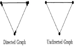
Figure 2.1: Directed and undirected graphs
Directed Graph
A directed graph is a graph in which every edge is a directed edge.
Undirected Graph
A undirected graph is a graph in which every edge is an undirected edge.
Multigraph
A multigraph is a graph in which there exists two vertices having two or more edges incident upon
both of them.
CHAPTER 2. DEFINITIONS 8
Let (v,w) is a directed edge,vis called the tail andwis called the head of the edge.
Path
LetGis a multigraph, a path inG v ∗
wis a sequence of vertices and edges leading fromvtow. A
path is simple if all its vertices are distinct. Verticesvandware called the terminating vertices of
the path.
Cycle
A pathv ∗
wis a cycle if all its edges are distinct and the only vertex that occurs exactly twice on
the path isv.
Connected Graph
An undirected multigraph is connected, if every pair of verticesvandwinGis connected by a path.
Subgraph
IfG(V,E) andG0=(V0,E0) are two multigraphs such thatV⊆V0andE⊆E0thenG0is a subgraph of G.
Bond
A multigraph having exactly two verticesv,wand one or more edges (v,w) is called a bond.
Directed Tree
A directed tree is a directed graph whose undirected version is connected and has a vertex, called
the root, which is the head of no edges and all vertices except the root are the head of exactly one edge.
Spanning Tree
IfGis a multigraph, a treeTis a spanning tree ofG, ifTis a subgraph ofGandTcontains all the
vertices ofG.
CHAPTER 2. DEFINITIONS 9
A connected multigraphGis biconnected if for each triple of distinct verticesv,wandainV, there is a pathP:vwsuch thatais not on the pathP.
Separation Point
If there is a distinct triplev,w,ain graphGsuch thatais on every pathvw,ais called a Separation
point (or an articulation point) of G.
Separation Pair
Leta,bbe a pair of vertices in a biconnected multigraphG. Suppose the edges ofGare divided into equivalence classesE1,E2,...,Ensuch that two edges which lie on a common path do not contain
any vertex ofa,bexcept as an endpoint are in the same class. These classes are called the separation
classes ofGwith respect toa,b. If there are at least two separation classes, thena,bis a separation
pair ofGunless:
(i) there are exactly two separation classes, and one class consists of a single edge, or
(ii) there are exactly three separation classes, each consisting of a single edge. In much simpler
words, a separation pair is a pair of vertices that their elimination will disconnect a biconneted graph.
Triconnected Graph
IfGis a biconnected multigraph such that it does not contain a separation pair, then G is triconnected.
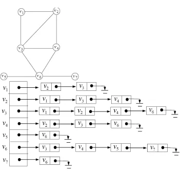
Adjacency List
In order to show the relation between the edges and vertices in a graph we can use an adjacency
list. This list shows which vertices are adjacent to a given vertexv.
CHAPTER 2. DEFINITIONS 10
Figure 2.2: A graph and its adjacency list
2.2
Depth-first Search
Depth-first search is a systematic method for exploring a multigraph[42]. This search can be used
for numbering the vertices in the graph and also determining a spanning tree of a graph.
In this search, first we assume that all the vertices are in theunvisitedstate. We start from an arbitrary
vertex, call it the root, and look at its adjacency list for unvisited vertices. If there are unvisited
vertices, we will arbitrarily choose one and move to that vertex. We continue the same process till
the time there are no unvisited vertices, then the search will backtrack. In depth-first search, each
edge is examined exactly twice and each vertex is visited once. If the graph is an undirected graph,
CHAPTER 2. DEFINITIONS 11
search numbers) and hence transform it to a directed graph.
The search can be presented as a recursive function as shown below:
DFS(v)
begin
visit vertexvand mark it asvisited
choose anunvisitedvertexwinA[v] (the adjacency list ofv)
invoke DFS(w)
end
It is well-known that depth-first search runs inO(|V|+|E|) time, whereEis the edge set andVis the
vertex set of the graph[42].
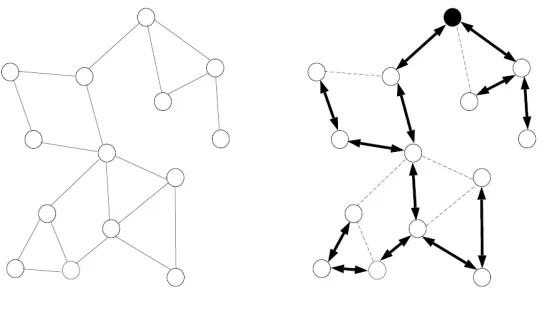
The following figures shows how a graph is traversed by DFS.
Figure 2.3: DFS traversal
As noted before, DFS can be used for constructing a spanning tree of a graph. After DFS is
applied, the edges that belong to the spanning tree are called thetree-edgesand the rest of the edges
are called the fronds. The difference between the tree edges and the fronds is that, if during the search we visit a vertexwinA[v] andwis not visited the edge (v,w) will become a tree-edge and if
CHAPTER 2. DEFINITIONS 12
2.2.1
Some Definitions Related To DFS
DFS Tree
The spanning tree constructed by the depth-first search traversal of the graph is called a DFS tree
of the graph.
DFS Number
The number assigned to a vertex during a depth-first search is called thedepth-first search numberof
that vertex and is denoted bydfs(v).
Child
In the DFS tree, if (v,w) theis a tree edge thenvis the parent of thewandwis a child ofv.
Leaf
If a vertex in the DFS tree of graphGdoes not have any children, it is a leaf.
Ancestor and descendant
In a DFS tree, ifd f s(v)<d f s(w) thenvis an ancestor ofwandwis a decendant of thev. Each node
is its own descendant and ancestor. The number of descendants of the nodevis denoted bynd(v).
Subtree
In the DFS treeT, a subtree rooted inw, denoted byT(w), is the largest subgraph ofT(which is a
tree) whose root isw.
Incoming and Outgoing frond
If (v,w) is a frond (also called back-edge) then it is an outgoing frond ofvand an incoming frond of
Chapter 3
Sequential Algorithm
3.1
The Sequential Algorithm Of Hopcroft And Tarjan
In 1973, Tarjan and Hopcoft presented a sequential algorithm for finding the triconnected
com-ponenets of a biconnected graph. The algorithm is based on depth-first search and makes several
passes over the input graph. Since we are focusing our algorithm on finding separation pairs,
there will be certain parts of their algorithm that we will not discuss in this thesis. However, we
will explain the sequential algorithm of Tarjan and Hopcroft to facilitate the understanding of our
distributed algorithm in the next chapters.
The algorithm basically consists of the following steps (these steps will be discussed in more detail
in the following sections):
1. The input graphGis split into a set of triple bonds and a graphG0.
2. IfG0is already biconnected, then continue at Step 3. Otherwise, decomposeG0into
bicon-nected components using the biconnectivity algorithm of Tarjan[20]. Repeat Step 3 and 4 for each
of the biconnected components.
3. Perform a depth-first search overG0
(or a biconnected component ofG0
) to create an adjacency
structure of the graph that complies with certain conditions (to be discussed in the following
sections).
CHAPTER 3. SEQUENTIAL ALGORITHM 14
4. Based on the adjacency structure, perform a depth-first search over G0
(or a biconnected
component ofG0
) to decompose the graph into a collection of paths.
5. For each of the paths determined in Step 4, determine a subset of separation pairs lying
on it. The separation pairs are identified by keeping track of two stacks one of which contains
the potential separation pairs and the other contains the edges of the split components. The split
components are determined along with the separation pairs.
6. The set of triple bonds and triangles are merged to form a set of bonds and polygons. These
bonds, polygons together with the split components form the triconnected components of the input
graphG.
3.2
A Characterization of Separation Pairs
Hopcroft et al. classify separation pairs into two types: Type-1 and Type-2. Furthermore, they give
the following characterization theorem of separation pairs (note that the vertices are presented by
their depth-first search numbers):
Theorem 13[20] Let G=(V,E) be a biconnected graph and a,b be two vertices inG with a<b. Then{a,b}is a separation pair if and only if one of the following conditions holds:
•Type-1: There are distinct verticesr,a,bands,a,bsuch thatb→r,lowpt1(r)=a,lowpt2(r)≥b
andsis not a decendant ofr.
•Type-2: There is a vertexr,bsuch thata→r{b,bis a first decendant ofr,a,1, every frond
xdywithr≤x<bhasa≤y, and every frondxdywitha<y<bandb→wdxhaslowpt1(w)≥a.
We shall use the graph given in Hopcroft et al. to illustrate various concepts and ideas. The graph
CHAPTER 3. SEQUENTIAL ALGORITHM 15
Figure 3.1: Separation pairs[20]
3.3
A High-level Description of the Algorithm
In the algorithm of Hopcroft et al., in order to find the triconnected components, the graph is split
into smaller graphs which are called the split graphs. For each separation pair (a,b), the graphG
is split into two graphsG1andG2and an virtual edge of (a,b) is added to the split graphs. If the
split graphs are split until no more splits are possible, the graphs remaining are called the split
components. These split components are non-unique.
There are three types of split components: triple bonds such as ({a,b},{(a,b),(a,b),(a,b)}), triangles
such as ({a,b,c},{(a,b),(a,c),(b,c)}) and a triconnected graphs.
Some of the split components are then reassembled (merged). Specifically, the triple bonds are
merged to form a set of bonds B and the triangles are merged to form polygonsP. The set of
BS
PS{
triconnecgtedgraphs}is the set of triconnected components of the input graphG. Note that
CHAPTER 3. SEQUENTIAL ALGORITHM 16
Basically, the algorithm of Hopcroft et al. can be summarized into the following steps:
• The multiple edges in the graphGare split offto form a set of triple bonds and a graphG0
• The biconnected components of G0
are determined and for each of them are processed as
follows:
1. The split components are determined;
2. Connected components are determined by combiningB,Pand the triconnecgted graphs.
The main part of the algorithm of Hopcroft et al. is to find the split components of the biconnected
components ofG0
. For this purpose, he had to determine the separation pairs of the graph. In order
to find the separation pairs, several passes are made over the graph and a few values are calculated
as follows:
• The graph is traversed with DFS andlowpt1(v),lowpt2(v),nd(v) andparent(v) are calculated;
• An acceptable adjacency list is constructed for each vertexv;
• A DFS is performed based on the acceptable adjacency list structure to partition the edges into
disjoint simple paths,lowpt1(v) andlowpt2(v) are recalculated andA1[v],degree(v) andHighpt
are calculated for each node.
During the first depth-first search, the following parameters are calculated for each vertexv:]nd(v)
(the number of descendants ofv),lowpt1(v) andlowpt2(v).
The definition forlowpt1(v) andlowpt2(v) are as follows:
lowpt1(v)=min({v}S{
lowpt1(w)|v
w} S{
w|v−
w})
and
lowpt2(v)=min({v}S
(({lowpt1(w)|v
w} S{
lowpt2(w)|v
w} S{
w|v−
CHAPTER 3. SEQUENTIAL ALGORITHM 17
In simple words,lowpt1(v) is the lowest vertex accessible tovby traversing zero or more tree-edges
and one frond andlowpt2(v) would be the second lowest vertex accessible tovin the graphGin the
same way.
Next, the order of the vertices adjacent tovinA[v] is changed. The resulting adjacency list,A(v) is
called anacceptableadjacency lists.A(v) is created based on the functionφ. It is defined as below:
ife=(v,w) is a tree edge andlowpt2(w)<v, thenφ(e)=2lowpt1(w) ife=(v,w) is a tree edge andlowpt2(w)≥v, thenφ(e)=2lowpt1(w)+1
ife=(v,w) is an outgoing frond, thenφ(e)=2w+1.
Next, another DFS is performed over the graph, this search will proceed according to the new
A(v) to generate a collection of paths. Specifically, whenever a tree-edge is encountered, it is added
to the path and whenever a frond is encountered, it will be the last edge in the path. The first path is
a cycle and the remaining paths are simple paths. Each path has its first and last vertex in common
with other paths. Becaue these paths are generated according to theacceptableadjacency list every
vertex will end in the lowest possible vertex.A1(v) is defined as the first vertex encountered in the
newA(v) andHighptis the first frond encountered during the path finding search. Since the paths
are found based on DFS they can be found inO(|V|+|E|) time.
Next, the separation pairs are determined based on the theorem stated at the beginning of this
chapter (which we restate below for convenience) and the values calculated above.
Theorem 13[20] Let G=(V,E) be a biconnected graph and a,b be two vertices inG with a<b. Then{a,b}is a separation pair if and only if one of the following conditions holds:
•Type-1: There are distinct verticesr,a,bands,a,bsuch thatb→r,lowpt1(r)=a,lowpt2(r)≥b
andsis not a decendant ofr.
•Type-2: There is a vertexr,bsuch thata→r{b,bis a first decendant ofr,a,1, every frond
xdywithr≤x<bhasa≤y, and every frondxdywitha<y<bandb→wdxhaslowpt1(w)≥a.
Two stacks are used, namelyESTACKandTSTACK.
CHAPTER 3. SEQUENTIAL ALGORITHM 18
vertex in the triconnected component. The algorithm checks the top entry on theTSTACKto see
if the condition given in Theorem 13 is satisfied. TheESTACKis used to keep the edges of split
components. The output of the algorithm is the separation pairs and the triconnected components
Chapter 4
The Distributed Model
A distributed network can be represented by an undirected graphG=(V;E) whereVis the set of network sites andEis the set of communication links. The sites communicate with each other by
sending messages over the communication links and performing some computations locally. Every
site has an identity and is able to keep data locally. Each site knows which other sites in the network
it is connected to. Without loss of generality, we assume that a message if sent will be delivered
and no message will be lost in the network. We also assume that it will take finite time for every
message to be delivered. Since communication cost is larger than local computation time by many
order of magnitude, we shall consider the time for local computations as negligible.
The message complexity of a distributed algorithm is the total number of messages sent when the
algorithm is executed. The time complexity of a distributed algorithm is the maximum time passed
between the beginning and end of the algorithm. For simplicity, it is commonly assumed that each
message will take at most one time unit to be delivered.
Since our distributed algorithm is bsed on an algorithm that uses depth-first search, we will need
to study distributed depth-fist search. There have been a number of DDFS algorithms presented
during the last two decades. These algorithms have different message lengths and different rules imposed on their networks. Some of the most important DDFS algorithms are presented by
Awer-buch[4], Cidon[12],Cheung[9], Lakshmanan et al.[29], Makki et al.[31] and Sharma et al.[39]. The
following table compares the time and message complexity of these algorithms:
CHAPTER 4. THE DISTRIBUTED MODEL 20
Table 4.1: Different DDFS algorithms and their complexities[47] Author Message length Time Mesage
Cheung O(1) 2m 2m
Awerbuch O(1) <4n 4m
Lakhamanan et al. O(1) 2n−2 ≤2m,<4m−(n−1)
Cidon(corrected) O(1) 2n−2 ≤2m,<4m−(n−1)
Tsin O(lgn) n(1+r) ≤n+1,<4m−(n−1)
Sharma et al. O(n) 2n−2 2n−2
Makki et al. O(n) n(1+r) n(1+r)
Some of the algorithms assume that every node in the network has access to global information
about all the other nodes in the network. This assumption will lower the number of messages
passed along the network substantially. The algorithms presented by Sharma et al. and Makki et
al. use such an assumption and use messages of lengthO(n). They show improvement in time or
message complexity compared to the other algorithms.
Other algorithms such as Cidon’s use messages of lengthO(1). Cidon’s algorithm also adopt a
weaker computer model in that it does not require the FIFO (First-in-first-out) rule, which means
that the messages are not processed in the order they arrived and are not delivered in the same
order they were received. In 2002, Tsin[47] presented two counterexamples to show that Cidon’s
algorithm does not always work correctly. He also showed how to correct the errors in Cidon’s
algorithm. We will base our distributed depth-fist search on the corrected Cidon’s algorithm
according to Tsin.
In summary, the following are the assumptions we make for our network model:
• All the messages sent over the links are delivered correctly in one time unit; each message
deliverance takes finite time and the FIFO rule is not required.
• Every node knows only its incident links and has no global knowledge of the network.
• the message length isO(log|V|).
• the nodes in the network run asynchronously (i.e. there is no clock synchronizing them).
Each node can be either in theidlestate ordiscoveredstate. The edges incident to every node can
CHAPTER 4. THE DISTRIBUTED MODEL 21
are markedunvisited. There are two types of messages, namelyVisitedandToken, for performing
thebasicdepth-first search. TheTokenis sent in sequential order from a node to one of its adjacent
nodes as the graph is being traversed by a depth-first search.
Initially, all the nodes are inidlestate. The distributed algorithm is invoked by one of the nodes.
After entering thediscoveredstate, the node chooses one of itsunvisitedlinks and sends theToken
over the link. It then marks the link aschild. The node also sends aVisitedmessage over every
incident link other than theparentlink to let the node at the end knows that it has been visited by
the search.
If a node receives aTokenmessage through anunvisited link, it will mark the link asparentand
enter thediscoveredstate, then it will pass theTokenalong one of itsunvisitedlinks. If there are no
unvisitedlinks left, then the search has to backtrack so theTokenis sent over theparentlink. This
process will continue until the search backtracks to the first node that initiated the DFS (which has
become the root of the DFS tree).
If the Token is sent through avisitedorunvisitedlink but not for the first time, the link is marked
asvisitedand no other action is taken. If aVisitedmessage is received through anunvisitedorchild
Chapter 5
The Distributed Algoithm
5.1
The Distributed Algorithm
We shall assume without loss of generality that the network is biconnected. If it is not, we can use
the existing distributed algorithm for biconnectivty to decompose the network into a collection of
biconnected networks and then apply our algorithm to each of them.
The algorithm is based on the sequential algorithm of Hopcroft and Tarjan. To carry the depth-first
search, we shall use the distributed depth-first search algorithm of Cidon with corrections made by
Tsin.
As with the algorithm of Hopcroft et. al., our algorithm makes three passes over the network
G=(V,E). During the first pass, a depth-first search is performed overGto generated a Palm tree
P=(V,EP) ofGandlowpt1(v),lowpt2(v),nd(v),v∈V, are computed. Usinglowpt1(v),lowpt2(v),v∈V,
the valuesφ(e),∀e∈E, is computed and the incident links of the Palm tree at each nodevare
rear-ranged to produce the acceptable adjacency structure,A(v),v∈V.
During this pass, the following types of messages are used:
Token(f lag,count,lowpt1,lowpt2,nd): when f lag=1, the message is sent to a child node; when
f lag=0, the message is sent to the parent node;countis the next depth-first search number avail-able for assigning to a node;lowpt1 andlowpt2 are thelowpt1 andlowpt2 values of the sender;ndis
CHAPTER 5. THE DISTRIBUTED ALGOITHM 23
the number of descendants of the sender.
Visited(d f s):d f sis the depth-first search number of the sender.
During the second pass, a depth-first search is made over the Palm tree P using the acceptable
adjacency structure andlowpt1(v),lowpt2(v),v∈Vare recomputed. The networkGis also implicitly
decomposed into a collection of paths,Pi,1≤i≤k, such thatP1is a cycle while eachPi,2≤i≤kis a
simple path whose terminating nodes lie on somePj,j<i.
During this pass, the following types of messages are used:
Token1(m): m is the parameter used in determining the new depth-first number during the
second pass (see Procedure 5 of[20]).
Visited: same as above.
During the third pass, a subset of separation pairs that are sufficient to decomposeGinto the split components are determined. The separation pairs are determined in parallel on the pathsPi,1≤i≤k.
During this pass, the following types of messages are used:
Vlink: to inform an ancestor of the sender to create a virtual link.
DecreaseDegree: to inform a descendant of the sender (which forms a Type-2 pair with the
sender) to update its degrees as well as creating a virtual link.
UpdateDegree: to inform an ancestor of the sender (which forms a Type-1 pair with the sender)
to update its degrees as well as creating a virtual link.
Deg of child is 2(f lag,f irstchild) with TSTACK: f lag=true if and only if the sender, say v, satisfies the condition: “deg(v)=2∧f irstchild(v)>v”. When f lag=true, f isrtchildis the first child
of the sender, it is irrelevant otherwise.
con-CHAPTER 5. THE DISTRIBUTED ALGOITHM 24
dition: “deg(v)=2∧f irstchild(v)>v”. When f lag=true, f isrtchildis the first child of the sender, it
is irrelevant otherwise. The receiver of the message isdwhich is an ancestor of the sender.
5.1.1
Determining
lowpt1,
lowpt2 and
nd(v)
Initially, all nodes are in theidlestate and all links are markedunvisited. One predesignated noder
then enters thediscoveredstate and initiates the algorithm by starting a depth-first search as follows:
d f s(r)←1;lowpt1(r)←lowpt2(r)←1; nd(r)←1;
callDFS(2);
send a messagevisit(1) over everyunvisitedincident link.
————————————————————————————————————
ProcedureDFS(count)
if(∃an incident linkethat is markedunvisited)then
sendToken(1,count,−,−,−) over linke;
mark linkeaschild;
else if(v=r)then/*vis the node executing algorithm DFS */ STOP
elsesendToken(0,count,lowpt1(v),lowpt2(v),nd(v)) over theparentlink;
————————————————————————————————————
At each nodev∈V, the following operations for computing the values oflowpt1(v),lowpt2(v),
andnd(v) are carried out:
•On receiving aToken(1,count,−,−,−) message from an incident link e:
if(state(v)=idle)then
state(v)←discovered;
mark linkeas theparentlink;
CHAPTER 5. THE DISTRIBUTED ALGOITHM 25
if(there is no savedvisitedmessage)then
lowpt1(v)←lowpt2(v)←d f s(v);
else
lowpt1(v)←min({d f s(w)|(visit(d f s(w)) is a saved message)∧(v,w),e} ∪{d f s(v)});
lowpt2(v)←min({d f s(w)|(visit(d f s(w)) is a saved message)∧(v,w),e} −{lowpt1(v)} ∪ {d f s(v)});
nd(v)←1;
call DFS(count+1);
send avisit(d f s(v)) message over everyvisitedorunvisitedincident link.
else if(linkeis markedunvisited)then
mark linkeasvisited
else if(linkeis markedchild)then
mark linkeasvisited;
/* aTokenmessage must have been sent over linkeearlier. Let it beToken(1,cnt,−,−,−). Then, re-transmit the message */
callDFS(cnt);
•Upon receiving avisited(w) message from an incident link e:
if(state(v)=idle)thensave the message
else if(eis marked ‘unvisited’)/* i.e.eis a back-edge */
then
mark linkeasvisited;
if(w<lowpt1(v))then
lowpt2(v)←lowpt1(v);
lowpt1(v)←w;
else if(lowpt1(v)<w<lowpt2(v))then
CHAPTER 5. THE DISTRIBUTED ALGOITHM 26
else if(linkeis markedchild)then
mark linkeasvisited;
/* aTokenmessage must have been sent over linkeearlier. Let it beToken(1,cnt,−,−,−). Then, re-transmit the message */
callDFS(cnt);
if(w<lowpt1(v))then
lowpt2(v)←lowpt1(v);
lowpt1(v)←w;
else if(lowpt1(v)<w<lowpt2(v))then
lowpt2(v)←w;
•On receiving aToken(0,cnt,L1,L2,nd) message from a linke:
/* Linkemust be achildlink */
if(L1<lowpt1(v))then/* Updatelowpt1(v),lowpt2(v) */
lowpt2(v)←min{lowpt1(v),L2};
lowpt1(v)←L1;
else if(L1=lowpt1(v))then
lowpt2(v)←min{lowpt2(v),L2};
elselowpt2(v)←min{lowpt2(v),L1};
nd(v)←nd(v)+nd;
callDFS(cnt)
Theorem 5.1When the depth-first search terminates at the root r, lowpt1(v);lowpt2(v);nd(v);∀v∈V,
are correctly computed.
CHAPTER 5. THE DISTRIBUTED ALGOITHM 27
Base case: Consider a leaf-nodev. Sincevhas no child nodes, all of the links incident on it are
either outgoing fronds or the parent link. Therefore,lowpt1(v) andlowpt2(v) are computed purely
based on theVisitedmessages. As a result,lowpt1(v) andlowpt2(v) are computed as:
lowpt1(v)
=min({d f s(v)} ∪ {d f s(w)|(v,→w)∈EP})
=min({d f s(v)} ∪ {lowpt1(w)|(v→w)∈EP} ∪ {d f s(w)|(v,→w)∈EP}) and
lowpt2(v)
=min({d f s(v)} ∪({d f s(w)|(v,→w)∈EP} − {lowpt1(v)}))
=min({d f s(v)} ∪(({d f s(w)|(v,→w)∈EP} ∪ {lowpt1(w)|(v→w)∈EP} ∪{lowpt2(w)|(v→w)∈EP})− {lowpt1(v)})).
Hence, bothlowpt1(v) andlowpt2(v) are computed correctly at every leaf-node. Furthermore,nd(v)
is correctly set to 1.
Induction hypothesis: Suppose for every nodewonlevel>k,lowpt1(w),lowpt2(w),nd(w) are
cor-rectly computed.
Induction step:Consider a nodevon levelk. For each frondv,→w, nodevreceivesd f s(w) through
the incident linke=(v,→w). Furthermore, by the induction hypothesis,lowpt1(w),lowpt2(w),nd(w)
are correctly computed for every child nodew. Sincelowpt1(w),lowpt2(w) are sent to nodevthrough
aTokenmessages, it is easily verified that the algorithm correctly computeslowpt1(v) as:
min({d f s(v)} ∪({lowpt1(w)|v→w} ∪ {d f s(w)|(v,→w)=e∈EP}))
andlowpt2(v) as:
min({d f s(v)} ∪(({lowpt1(w)|v→w} ∪ {lowpt2(w)|v→w} ∪ {d f s(w)|(v,→w)=e∈EP})− {lowpt1(v)})).
Furthermore, it is easily verified thatnd(v) is correctly computed asP{
nd(w)|v→w}+1.
CHAPTER 5. THE DISTRIBUTED ALGOITHM 28
all the split components of the network. The separation pairs are determined based on Lemma 3 of
Gutwenger et. al., or originally, Lemma 13 of Hopcroft et. al.
Theorem 5.2 The distributed algorithm takes O(|V|) time and transmits O(|E|) messages to compute
lowpt1(v),lowpt2(v),nd(v),∀v∈V.
Proof: The algorithm performs a depth-first search over the networkG. Since the computation of
lowpt1(v),lowpt2(v),nd(v),v∈V, are done locally at each nodev, the computation thus takeszerotime.
The total time and message complexities are thus that same as those of the distributed depth-first
search algorithm which areO(|V|) andO(|E|), respectively[47].
5.1.2
Constructing the acceptable adjacency structure
At the end of the depth-first search during the first pass, the adjacency list for the palm tree at every
node is rearranged and the nodes are renumbered with new depth-first search numbers so that the
following properties are satisfied:
(i) the root of the depth-first treeTis numbered 1;
(ii) letv∈Vandwi,1≤i≤n, be its children inT. Then
d f s(wi)=d f s(v)+Pn
j=i+1nd(wj)+1;
(iii) For eachv∈V, the edgesein the adjacency list of v,A(v), are in ascending order according
tolowpt1(w) ife=v→w, orwife=v,→w, respectively. Moreover, letwi,1≤i≤n, be the
children ofv. Then∃i0such thatlowpt2(w)<d f s(v),1≤i≤i0andlowpt2(w)≥d f s(v),i0<i≤n.
Every frond inA(v) comes in betweenv→wi
0andv→wi0+1.
At each nodev, the links of the palm tree incident onvare ordered according to the following value:
∀e∈E,φ(e)=
CHAPTER 5. THE DISTRIBUTED ALGOITHM 29
ife=(v,w) is an outgoing frond, thenφ(e)=3w+2.
Definition: The adjacency structure for the palm tree, P=(V,EP), of the network G=(V,E) is
acceptableif for everyv∈V, the edgesein the adjacency list ofvare ordered according to increasing
value ofφ(e).
Note that the acceptable adjacency structure involves thechildlinks and theoutgoing non-treelinks
(linkse=v,→wsuch thatd f s(v)>d f s(w)) ofGonly.
At every nodev,v∈V, the following operations are performed:
callCompute phi(v);
Create the acceptable adjacency structure,A(v),v∈V, usingφ(e),e∈E.
————————————————————————————————————
ProcedureCompute phi(v);
————————————————————————————————————
for each(e∈A(v))do
if(e=v→w)then /*eis a tree link */
if(lowpt2(w)<v)then
φ(e)←3∗lowpt1(w)
elseφ(e)←3∗lowpt1(w)+2
else/*eis a frond */
φ(e)←3∗lowpt1(w)+1
————————————————————————————————————
CHAPTER 5. THE DISTRIBUTED ALGOITHM 30
5.1.3
Recalculating
dfs(v),
lowpt1(v),
lowpt2(v)
During the second pass, a depth-first search is performed over the palm tree,P=(V,EP) of the net-workG=(V,E) using the acceptable adjacency structureA(v),v∈V, ofPand renumber the nodes
with depth-first search numbers.
When the first pass was completed, all the nodes re-entered theidlestate. The root of the
depth-first search treerinitiates the second pass as follows:
state(r)←discovered;
m← |V|;
next←0;
highpt(r)←0;
newds f(r)←1 /* which ism−nd(r)+1 */;
callPathsearch(next,m,r);
send avisited(newd f s(r)) message over everyoutgoingnon-tree link.
————————————————————————————————————
ProcedurePathsearch(next,m,v)
next←next+1;
while((A(v)[next] is a non-tree link)∧(next≤deg(v)))do/* skip non-tree links */
next←next+1;
if(next≤deg(v))then
sendToken1(m) over the child linke, wheree=A(v)[next];
elsed f s(v)←newd f s(v); /* updated f s(v) */
if(v=r)then/*vis the node executing algorithm DFS */ STOP
elsem←m−1;
CHAPTER 5. THE DISTRIBUTED ALGOITHM 31
————————————————————————————————————
At each nodev∈V, the following operations for computing the values oflowpt1(v),lowpt2(v), and
nd(v) are carried out:
•On receiving aToken1(m) message from the parent link:
state(v)←discovered;
next←0;
highpt(r)←0;
newds f(v)←m−nd(v)+1;
callPathsearch(next,m,v);
send avisit(newd f s(v)) message over everyoutgoing non-treelink.
•On receiving avisited(w) message from an incident linke:
/* the linkemust be an incoming non-tree link */
highpt(v)←max{highpt(v),w};
•On receiving aToken1(m) message from achildlinke:
callPathsearch(next,m,v)
Theorem 5.3When the depth-first search terminates at the root r, d f s(v),highpt(v),∀v∈V, are correctly
computed.
Proof: The distributed algorithm performs a depth-first search over the networkGto re-calculate
d f s(v),v∈V. The correctness of computingd f s(v),v∈V, thus follows from that given in[47].
The correctness of computinghighpt(v),v∈Vfollows from that given in[20].
CHAPTER 5. THE DISTRIBUTED ALGOITHM 32
d f s(v),highpt(v),∀v∈V.
Proof:Same as that of Theorem 5.2.
After re-computingd f s(v)∀v∈V, another depth-first search is performed over the networkGto
re-calculatelowpt1(v),lowpt2(v),∀v∈V. Since the detail of the algorithm, the correctness proof and
the time and message complexity analysis are essentially the same as those for the first pass, we
shall omit them here. Instead, we state the following theorem.
Theorem 5.5The distributed algorithm takes O(|V|) time and transmits O(|E|) messages to re-compute
lowpt1(v),lowpt2(v),∀v∈V.
Proof:Immediate.
5.1.4
Determining the Separation Pairs
For ease of explanation, we shall usevandd f s(v) interchangeably in this section. During the third
pass, the algorithm finds a subset of separation pairs that are sufficient to generate all the split components of the network. The separation pairs are determined based on Lemma 3 of Gutwenger
et. al., or originally, Lemma 13 of Hopcroft et. al.
The third pass is initiated by all those nodes that have an outgoing non-tree link which is the last
link of a path. It goes as follows:
if(A(v)[1] is an outgoing non-tree link)then
/* The outgoing non-tree link is the last link of a path. */
TSTACK←null;
v.link←v.parent←null;/* initialize the virtual links */
A(v)←A(v)−A(v)[1]; /* exclude the last link from further consideration */
CHAPTER 5. THE DISTRIBUTED ALGOITHM 33
sendTSTACKand adeg of child is 2(false,null) message over theparentlink;
————————————————————————————————————
ProcedureUpdate-TSTACK(v)
————————————————————————————————————
for each(e∈A(v))do
if(e=v→w)then/*eis a tree link */
while(top entry (h,a,b) onTSTACKsatisfiesa>lowpt1(w))do
popTSTACK;
if(no entry was popped out ofTSTACK)then
push(w+nd(w)−1,lowpt1(w),v) ontoTSTACK
else
let (h0, a0,
b0
) be the last entry popped;
push(max{y,w+nd(w)−1},lowpt1(w),b0) ontoTSTACK;
elselete=v,→w;/*emust be a frond */
while(top entry (h,a,b) onTSTACKsatisfiesa>d f s(w))do popTSTACK;
if(no entry was popped out ofTSTACK)then
push(v,w,v) ontoTSTACK
else
y←max{h|(h,a,b)was popped out ofTSTACK};
let (h0,a0,b0) be the last entry popped;
push(y,w,b0) ontoTSTACK
rof;
CHAPTER 5. THE DISTRIBUTED ALGOITHM 34
————————————————————————————————————
ProcedureType-2(f lag,z)
————————————————————————————————————
if(f lag=true)then/* i.e. (deg(w)=2∧f irstchild(w)>w) */
mark (v,z) as a type-2 separation pair; /*z=f irstchild(w) */
v.child(v)←z; /*effectively deleted (v,w) and (w,f irstchild(w)) */
send avlink(v,z) message over the link (v,w);
else if(top entry(h,a,b)on TSTACK satis f ies a=v)then poptop-entry (h,a,b) out ofTSTACK;
mark (a,b) as a type-2 separation pair;
for each(e=(v,x)∈Ev)do
if(a≤x≤h)then
deg(v)←deg(v)−1; Ev←Ev− {e};
/* Join nodesv(=a) andbwith a virtual link (v,b) */
v.child(v)←b;deg(v)←deg(v)+1;Ev←Ev∪ {(v,b)};
send aDecreaseDegree(b,a,h) message to nodeb
————————————————————————————————————
————————————————————————————————————
ProcedureType-1
————————————————————————————————————
mark (v,lowpt1(w)) as a type-1 pair;
for each(e=(v,x)∈Ev)do
if(w≤x≤w+nd(w)−1)then
deg(v)←deg(v)−1;Ev←Ev− {e};
v.parent←lowpt1(w);Ev←Ev∪ {(v,lowpt1(v))};deg(v)←deg(v)+1;
![Figure 3.1: Separation pairs[20]](https://thumb-us.123doks.com/thumbv2/123dok_us/1462967.1179246/25.612.177.348.109.361/figure-separation-pairs.webp)
![Table 4.1: Different DDFS algorithms and their complexities[47]AuthorMessage lengthTimeMesage](https://thumb-us.123doks.com/thumbv2/123dok_us/1462967.1179246/30.612.158.492.146.251/table-dierent-ddfs-algorithms-complexities-authormessage-lengthtimemesage.webp)