INVESTIGATION
Modeling Causality for Pairs of Phenotypes
in System Genetics
Elias Chaibub Neto,* Aimee T. Broman,†Mark P. Keller,†Alan D. Attie,†Bin Zhang,* Jun Zhu,* and Brian S. Yandell‡,1
*Sage Bionetworks, Seattle, Washington 98109, and†Department of Biochemistry and‡Department of Statistics and Department of Horticulture, University of Wisconsin, Madison, Wisconsin 53706
ABSTRACTCurrent efforts in systems genetics have focused on the development of statistical approaches that aim to disentangle causal relationships among molecular phenotypes in segregating populations. Reverse engineering of transcriptional networks plays a key role in the understanding of gene regulation. However, transcriptional regulation is only one possible mechanism, as methylation, phosphorylation, direct protein–protein interaction, transcription factor binding, etc., can also contribute to gene regulation. These additional modes of regulation can be interpreted as unobserved variables in the transcriptional gene network and can potentially affect its reconstruction accuracy. We develop tests of causal direction for a pair of phenotypes that may be embedded in a more
complicated but unobserved network by extending Vuong’s selection tests for misspecified models. Our tests provide a significance
level, which is unavailable for the widely used AIC and BIC criteria. We evaluate the performance of our tests against the AIC, BIC, and a recently published causality inference test in simulation studies. We compare the precision of causal calls using biologically validated causal relationships extracted from a database of 247 knockout experiments in yeast. Our model selection tests are more precise, showing greatly reduced false-positive rates compared to the alternative approaches. In practice, this is a useful feature since follow-up studies tend to be time consuming and expensive and, hence, it is important for the experimentalist to have causal predictions with low false-positive rates.
A
key objective of biomedical research is to unravel thebiochemical mechanisms underlying complex disease traits. Integration of genetic information with genomic, pro-teomic, and metabolomic data has been used to infer causal
relationships among phenotypes (Schadtet al.2005; Liet al.
2006; Kulp and Jagalur 2006; Chen et al.2007; Zhuet al.
2004, 2007, 2008; Atenet al.2008; Liuet al.2008; Chaibub
Netoet al. 2008, 2009; Winrowet al.2009; Millsteinet al.
2009). Current approaches for causal inference in systems
genetics can be classified into whole network scoring
meth-ods (Zhuet al.2004, 2007, 2008; Liet al.2006; Liuet al.
2008; Chaibub Netoet al.2008, 2010; Winrowet al.2009;
Hagemanet al.2011) or pairwise methods, which focus on
the inference of causal relationships among pairs of
pheno-types (Schadt et al.2005; Liet al.2006; Kulp and Jagalur
2006; Chen et al. 2007; Aten et al. 2008; Millstein et al.
2009; Liet al.2010; Duarte and Zeng 2011). In this article
we develop a pairwise approach for causal inference among pairs of phenotypes.
Two key assumptions for causal inference in systems genetics are genetic variation preceding phenotypic variation and Mendelian randomization of alleles in unlinked loci. These conditions together, which provide temporal order and eliminate confounding of other factors, justify causal claims between QTL and phenotypes. Causal inference among
phenotypes is justified by conditional independence relations
under Markov properties (Liet al.2006; Chaibub Netoet al.
2010).
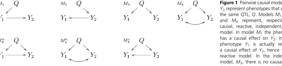
Given a pair of phenotypes,Y1andY2, that co-map to the
same quantitative trait locus,Q, our objective is to learn which
of the four distinct models,M1,M2,M3, andM4, depicted in
Figure 1, is the best representation for the true relation
be-tweenY1andY2. ModelsM1,M2,M3, and M4represent,
re-spectively, the causal, reactive, independence, and full models as collapsed versions of more complex regulatory networks. Copyright © 2013 by the Genetics Society of America
doi: 10.1534/genetics.112.147124
Manuscript received October 24, 2012; accepted for publication December 6, 2012 Available freely online through the author-supported open access option.
Supporting information is available online athttp://www.genetics.org/lookup/suppl/
doi:10.1534/genetics.112.147124/-/DC1.
1Corresponding author: Department of Statistics, University of Wisconsin, 1300
University Ave., Madison, WI 53706. E-mail: [email protected]
For instance, when the data are transcriptional and one gene is upstream of other genes, the regulation of the up-stream gene may affect those downup-stream, even when the regulation takes place via post-transcriptional mechanisms and, hence, is mediated by unobserved variables. Tran-scriptional networks should be interpreted as collapsed versions of more complicated networks, where the pres-ence of an arrow from a QTL to a phenotype or from one phenotype to another simply means that there is a
direc-tional influence of one node on another (that is, there is at
least one path in the network where the node in the tail of
the arrow is upstream of the node in the head).Supporting
Information,Figure S1shows a few examples of networks and their collapsed versions. Our goal in this article is to infer the causal direction between two nodes, and the term
“causal”should be interpreted as causal direction, meaning
either direct or indirect causal relations.
In this article, we propose novel causal model selection hypothesis tests and compare their performance to the AIC and BIC model selection criteria and to a causality inference
test (CIT) proposed by Millsteinet al.(2009). AIC (Akaike
1974) and BIC (Schwarz 1978) are widely used penalized likelihood criteria performing model selection among mod-els of different sizes. Overparameterized modmod-els tend to
overfit the data and, when comparing models with different
dimension, it is necessary to counterbalance model fit and
model parsimony by adding a penalty term that depends on the number of parameters. CIT is an intersection-union test, in which a number of equivalence and conditional F tests are
conservatively combined in a single test.P-values are
com-puted for modelsM1andM2in Figure 1, but not for theM3
orM4models, and the decision rule for model calling goes as
follows: (1) callM1if theM1P-value is less than a signifi
-cance thresholdaand theM2P-value is greater thana; (2)
call M2 if it is the other way around; (3) call Mi if both
P-values are greater thana; and (4) make a“no call”if both
P-values are less thana. TheMicall actually means that the
model is notM1orM2and could correspond to anM3orM4
model. Note that the CIT makes a no call when bothM1and
M2models are simultaneously significant.
Our causal model selection tests (CMSTs) adapt and
extend Vuong’s (1989) and Clarke’s (2007) tests to the
com-parison of four models. Vuong’s model selection test is a
for-mal parametric hypothesis test devised to quantify the uncertainty associated with a model selection criterion, com-paring two models based on their (penalized) likelihood scores. It uses the (penalized) log-likelihood ratio scaled by its standard error as a test statistic and tests the null hypothesis that both models are equally close to the true data generating process. While the (penalized) log-likelihood scores can determine only whether, for example, model A
fits the data better than model B, Vuong’s test goes one step
further and attaches aP-value to the scaled contrast of
(pe-nalized) log-likelihood scores. In this way it can interrogate
whether the betterfit of model A compared to model B is
statistically significant. Vuong’s test tends to be conservative
and low powered. Clarke (2007) proposed a nonparametric version that achieves an increase in power at the ex-pense of higher miss-calling error rates by using the median rather than the mean of (penalized) log-likelihood ratio.
We propose three distinct versions of causal model selection tests: (1) the parametric CMST test, which corresponds to an intersection-union test of six separate
Vuong’s tests; (2) the nonparametric CMST test, constructed
as an intersection-union test of six of Clarke’s tests; and (3)
the joint-parametric CMST test, which mimics an intersection-union test and is derived from the joint distribution of
Vuong’s test statistics. These CMST tests inherit from
Vuong’s test the property that none of the models being
compared need be correct. That is, the true model may de-scribe a more complicated network, including unobserved factors. Our approach simply selects the wrong model that is closest to the (unknown) true model.
Methods
Vuong’s model selection test
The Kullback–Leibler Information Criterion (KLIC) (Kullback
1959) measures the closeness of a probability model to the true distribution of data. Sawa (1978) showed that the KLIC orders approximate models by comparing the expected value of the log likelihood under the true model. Vuong (1989) used this result to develop an empirical test of two models based on the sample mean of the log-likelihood ratio scaled by its sample standard error.
Formally, {f(y|x; u) : u 2 Q} represents a parametric
family of conditional models and
KLICh0;f¼E0log h0ðyjxÞ2E0½log fðyjx;u*Þ
¼
Z
x
Z
yh
0ðyjxÞlog h0ðyjxÞ
fðyjx;u*Þdy
#
h0ðxÞdx;
(1)
whereE0represents the expectation with respect to the true
joint distribution h0(y,x) =h0(y|x)h0(x), and u
*is the
pa-rameter value that minimizes the KLIC distance fromfto the
true model (Sawa 1978). Note thatfneed not belong to the
same parametric family as h0.
A modelf1(y|x;u1*), denotedf1for short, is regarded as
a better approximation to the true modelh0(y|x), than the
alternative model f2(y|x; u2*) if and only if KLIC(h0; f1)
,KLIC(h0;f2), or alternatively,E0[logf1].E0[logf2] (Sawa
1978). Vuong’s model selection test is based on the latter
criterion and the null and alternative hypotheses are defined
as
H0:E0½LR12 ¼0; H1:E0½LR12.0; H2:E0½LR12,0;
(2)
whereLR12= logf12logf2. The null hypothesis isf1andf2
are equally close to the true distribution. The alternative
hypothesisH1means thatf1is better thanf2and conversely
for the alternativeH2.
The quantity E0[LR12] is unknown, but under fairly
general conditions the sample mean and variance of
LR12^ ;i¼log ^f1;i2log ^f2;i converge almost surely to
E0[LR12] andVar0[LR12] = s
12.12, where^f1;i¼f1ðyijxi; ^u1Þ
and ^u1 is the maximum-likelihood estimate of u1 (Vuong
1989). LetL^R12¼Pni¼1L^R12;i, then, underH0,
n21=2L^R12= ffiffiffiffiffiffiffiffiffiffiffiffiffis^12:12
p
/d
Nð0;1Þ: (3)
Under H1 this test statistic converges almost surely to N,
whereas, underH2, it converges to2N(Vuong 1989).
Vuong’s test is based on the unadjusted log-likelihood
ratio statistic. However, competing models may have different dimensions, requiring a complexity penalty. The penalized
log-likelihood ratio is given by LR^*12¼L^R122D12, where
the penaltyD12is the difference of the number of parameters
between models 1 and 2 (for AIC) or this value rescaled by
(logn)/2 (for BIC). Because the penalty term is of smaller
size thann1/2, the adjusted log-likelihood ratio accounting for
different model dimensions
Z12¼n21=2LR^*12=
ffiffiffiffiffiffiffiffiffiffiffiffiffi
^
s12:12
p
(4)
has the same asymptotic properties as n21=2L^R12= ffiffiffiffiffiffiffiffiffiffiffiffis^
12:12
p
(Vuong 1989).
TheP-value of Vuong’s test is given byp12=P(Z12$z12) =
12F(z12), whereF() represents the cumulative density
func-tion of a standard normal variable (Vuong 1989). Note that
sinceZ12=2Z12;p21= 12F(z21) =F(z12), so thatp12+
p21 = 1. This property of the Vuong’s test ensures that the
P-values of the intersection-union tests cannot be
simulta-neously significant.
Figure S2illustrates how Vuong’s test trades a reduc-tion in false positives against a reducreduc-tion in statistical power. In our applications we need to account for both nested and nonnested models. While the presented test
corresponds to Vuong’s test for strictly nonnested
mod-els, it is also valid for nested models when we adopt
penalized likelihood scores (see File S1, for further
details).
Clarke’s model selection paired sign test
The model selection paired sign test (Clarke 2007) is a
non-parametric alternative to Vuong’s test, testing the null
hy-pothesis that the median log-likelihood ratio is 0. Clarke’s
test statistic, T12, is a sign test on L^R12;i. Under the null
hypothesis that the median log-likelihood ratio is zero,T12
has a binomial distribution, and theP-value for comparing
models 1 and 2 is
p12¼PðT12$t12Þ ¼
Xn
k¼t12
Ckn22n; (5)
withCn
k ¼n!=k!ðn2kÞ!. TheP-values forT12andT21do not
add to 1 since the statistics are discrete,
p12þp21¼1þCn
t122
2n. Nonetheless, the Cn
t122
2n term
decreases to 0 asnincreases, and, in practice,p12+p21
1 even for moderate sample sizes. We adjust this test using
the AIC or BIC penaltyD12,
T12¼
Xn
i¼1
11 n
L^R12;i2n21D12.0
o
; (6)
to account for the varying dimensionality of the models.
Causal model selection tests
The four modelsM1,M2,M3, andM4(Figure 1) are used to
derive intersection-union tests based on the application of
six separate Vuong (or Clarke) tests comparing, namely,f1·
f2,f1·f3,f1·f4,f2·f3,f2·f4, andf3·f4. Sunet al.(2007)
implicitly used intersection unions of Vuong’s tests to select
among three nonnested models. Here, we present three dis-tinct versions of the CMST: (1) parametric, (2) nonparamet-ric, and (3) joint-parametric CMST tests. We implement the tests with penalized log likelihoods, but state results for log likelihoods.
Here we focus on model M1andP-valuep1, with
analo-gous results and notation for the other three models.
Start-ing with the parametric version, we test the nullH0: model
M1is no closer to the true model thanM2,M3orM4, against
the alternative H1:M1is closer to the true model thanM2,
M3, andM4. More explicitly, we test,
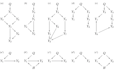
Figure 1 Pairwise causal models.Y1and Y2represent phenotypes that co-map to the same QTL,Q. ModelsM1,M2,M3, and M4 represent, respectively, the causal, reactive, independent, and full model. In modelM1the phenotypeY1 has a causal effect onY2. In M2, the phenotype Y1 is actually reacting to a causal effect ofY2, hence the name reactive model. In the independence model,M3, there is no causal relation-ship betweenY1andY2and their corre-lation is solely due toQ. The full model,M4, corresponds to three distribution equivalent modelsMa4,Mb4, andMc4which cannot be distinguished as their maximized-likelihood scores are identical. Model Mb4 represents a causal independence relationship where the correlation betweenY1 andY2 is a consequence of latent causal phenotypes, common causal QTL, or of common environmental effects. ModelsMa4andM4ccorrespond to causal-pleiotropic and reactive-causal-pleiotropic relationships, respectively.
H0:
E0½LR12 ¼0 [
E0½LR13 ¼0 [
E0½LR14 ¼0 ;
(7)
against
H1:
E0½LR12.0 \
E0½LR13.0 \
E0½LR14.0 :
(8)
The rejection region for this test is min{z12,z13,z14} . ca,
where ca is the a-critical value of the standard normal.
The intersection-union P-value is p1 = max{p12, p13,p14}.
For anya, ifp1# a, then min{p2,p3,p4}$12a. Therefore,
the proposed CMST test has at most one significant model
P-value at a time, in contrast to the CIT approach.
The nonparametric CMST test corresponds to an
intersec-tion union of Clarke’s tests, exactly analogous to the
paramet-ric version. Because in practicep12+p211 for Clarke’s test,
the nonparametric CMST test also does not allow the
detec-tion of more than one significant modelP-value.
Simple application of separate Vuong tests overlooks the dependency among the test statistics. A multivariate exten-sion, the joint parametric CMST test, can be developed to
address this caveat. For model M1, and under the same
general regularity conditions of Vuong (1989), the sample
covariance of LR12^ ;i and LR13^ ;i, s^12:13, converges almost
surely to Cov0[LR12, LR13] = s
12.13 (and similarly for all
other covariance terms). Therefore, the sample covariance
matrix,S^1, converges almost surely toS1. From the
multi-variate central limit and Slutsky’s theorems (Shao 2003), if
0 @E
0½LR 12
E0½LR13
E0½LR14
1
A¼
0 @00
0 1
A (9)
then Z1¼diagðS^1Þ2
1= 2LR^
1= ffiffiffin
p
/dN3ð0;r
1Þ; where LR^1¼
ðL^R12;LR13^ ;LR14^ ÞT and r1¼diagðS1Þ2
1= 2S
1diagðS1Þ2
1= 2 is
the correlation matrix
r1¼
0
@r121:13 r121:13 rr1312::1414
r12:14 r13:14 1
1
A: (10)
The condition in (9) is the worst case of the more general
null hypothesis thatM1is not better than at least one ofM2,
M3,M4, or
H0: min
E0½LR12;E0½LR13;E0½LR14 #0: (11)
We test this against the alternative thatM1is better than all
three, or
H1: min
E0½LR12;E0½LR13;E0½LR14 .0; (12)
using the statisticW1= min{Z1}, withP-value
PðW1$w1Þ ¼PðminfZ12;Z13;Z14g$w1Þ
¼PðZ12$w1;Z13$w1;Z14$w1Þ: (13)
The joint-parametric CMST test withW1follows the spirit of an
intersection union test while accounting for dependency among test statistics. Table 1 depicts the joint CMST tests for all models. The CMST tests are implemented in the R/qtlhot package available at CRAN. Although not explicitly stated in the notation, the pairwise models can easily account for additive and interactive covariates, and our code already implements this feature. When using this package please cite this article.
Simulation studies
We conducted two simulation studies. In the first “pilot
study,” we focus on performance comparison of the AIC,
BIC, CIT, and CMST methods with data generated from simple causal models. The goal is to understand the
behav-ior of our methods in diverse settings. In the second“
large-scale study,”we perform a simulation experiment, with data
generated from causal models emulating QTL hotspot pat-terns. The goal is to understand the impact of multiple test-ing on the performance of our causality tests.
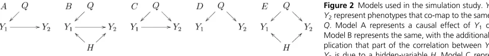
The pilot simulation study has data generated from models A to E in Figure 2. We conducted 10 simulation
studies, generating data from the five models described
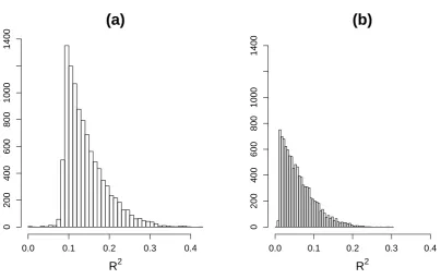
above under sample sizes 112 (the size of our real data example) and 1000. For each model, we simulated 1000 backcrosses. We chose simulation parameters to ensure that
99% of the R2 coefficients between phenotypes and QTL
ranged between 0.08 and 0.32 for the simulations based on sample size of 112 subjects and between 0.01 to 0.20
for the simulations based on 1000 subjects (seeFile S2,File
S3, and File S4 for details). We evaluated the method’s
performance using statistical power, miss-calling error rate, and precision. These quantities were computed as,
Power¼TP
N; Miss-calling error¼
FP
N;
Precision¼ TP
TPþFP;
whereNis the total number of tests, and TP (true positives)
and FP (false positives) are defined according to Table 2,
which depicts possible calls against simulated models and
tabulates whether a specific call correctly represents the
Table 1 Model selection tests for modelsM1,M2,M3, andM4
H0 Null distribution P-value
H0M1 Z
1¼ ðZ12;Z13;Z14ÞTN3ð0;r1Þ^ p1=P(Z12$w1,Z13$w1,Z14$w1)
H0M2 Z
2¼ ðZ21;Z23;Z24ÞTN3ð0;r2^ Þ p2=P(Z21$w2,Z23$w2,Z24$w2)
H0M3 Z
3¼ ðZ31;Z32;Z34ÞTN3ð0;r3^ Þ p3=P(Z31$w3,Z32$w3,Z34$w3)
H0M4 Z
4¼ ðZ41;Z42;Z43ÞTN3ð0;r4^ Þ p4=P(Z41$w4,Z42$w4,Z43$w4)
Herewk= min{zk} fork =1,...,4, andrkis defined in analogy withr1in Equation 10.
causal relationship between the phenotypes in the model from which the data were generated.
In the large-scale simulation study we investigate the empirical FDR (1 minus the precision) and power levels achieved by the CMST tests using the Benjamini and Hochberg (1995) and the Benjamini and Yekutieli (2001) FDR control procedures (denoted, respectively, by BH and BY), as well as no multiple testing correction. We simulate data from the models in Figure 3, which emulate eQTL
hot-spot patterns, i.e., genomic regions to which hundreds or
thousands of traits co-map (Westet al.2007). In each
sim-ulation we generated 1000 distinct backcrosses with pheno-typic data on 5001 traits on 112 individuals. We simulated
unequally spaced markers for model F, but equally spaced
markers forG, withQ1andQset 1 cM apart. Because wefit
almost three million hypothesis tests in this simulation study, we did not include the CIT tests in this investigation,
restricting our attention to the computationally more effi
-cient CMST tests. The details for our choice of simulation
parameters and QTL mapping are presented inFile S2,File
S3, andFile S4. A frequent goal in eQTL hotspots studies is
to determine a master regulator,i.e., a transcript that
reg-ulates the transcription of the other traits mapping to the
hotspot. A promising strategy toward this end is to test thecis
traits (i.e., transcripts physically located close to the QTL
hotspot) against all other co-mapping traits. Our simula-tions evaluate the performance of the CMST tests in this setting.
Results
Pilot simulation study results
Figure 4 depicts the power, miss-calling error rate, and pre-cision of each of the methods based on the simulation results
of allfive models in Figure 2. The results of the AIC and BIC
approaches are constant across all significance levels since
these approaches do not provide a measure of statistical
significance. For those methods, we simply fit the models
to the data and select the model with the best (smallest) score.
Overall, the AIC, BIC, and CIT showed high power, high miss-calling error rates, and low precision. The CMST methods, on the other hand, showed lower power, lower miss-calling error rates, and higher precision. The non-parametric CMST tended to be more powerful but less precise than the other CMST approaches. As expected, for
sample size 1000, all methods showed an increase in power and precision and decrease in miss-calling error rate.
Figure S3,Figure S4,Figure S5,Figure S6, andFigure S7
show the simulation results data for each one of models A to
E, when sample size is 112. Figure S8, Figure S9, Figure
S10,Figure S11, andFigure S12show the same results for sample size 1000. Some of the simulated models were in-trinsically more challenging than others. For instance, in the absence of latent variables the causal and independence relations can often be correctly inferred by all methods
(see the results for models A and D in Figure S3, Figure
S6, Figure S8, and Figure S11). However, the presence of hidden variables in models B and E tend to complicate mat-ters. Nonetheless, although the AIC, BIC, and CIT methods tend to detect false positives at high rates in these compli-cated situations, the CMST tests tend to forfeit making calls
and tend to detect fewer false positives (seeFigure S4,Figure
S7,Figure S9, andFigure S12). Model C is particularly
chal-lenging (Figure S5 and Figure S10), showing the highest
false-positive detection rates among all models.
In genetical genomics experiments we often restrict our
attention to the analysis ofcis-genes againsttrans-genes. In
this special case it is reasonable to expect the pleiotropic
Figure 2 Models used in the simulation study.Y1and Y2represent phenotypes that co-map to the same QTL, Q. Model A represents a causal effect ofY1on Y2. Model B represents the same, with the additional com-plication that part of the correlation betweenY1and Y2is due to a hidden-variableH. Model C represents a causal-pleiotropic model, whereQaffects bothY1andY2butY1also has a causal effect onY2. Model D shows a purely pleiotropic model, where both Y1andY2are under the control of the same QTL, but one does not causally affect the other. Model E represents the pleiotropic model, where the correlation betweenY1andY2is partially explained by a hidden-variableH.
Table 2 True and false positives
CMST Model A Model B Model C Model D Model E
M1 TP TP FP FP FP
M2 FP FP FP FP FP
M3 FP FP FP TP FP
M4 FP FP TP FP TP
CIT Model A Model B Model C Model D Model E
M1 TP TP FP FP FP
M2 FP FP FP FP FP
Mi FP FP TP TP TP
Each entryi,jrepresents whether the call on rowiis a true positive (TP) or as false
positive (FP), when the data are generated from the model on columnj. For
in-stance, when data are generated from models A or B, aM1call represents a true
positive, whereas aM2,M3, orM4call represents a false positive for the AIC, BIC,
and CMSTs approaches (for the CIT aM2orMicall represents false positive). Note
that aM4call is considered a true positive for model C (in addition to model E)
because it corresponds to modelMa
4on Figure 1 and, hence, is distribution
equiv-alent to modelM4. Please note too that because the CIT provides P-values for only
theM1andM2calls, but not for theM3andM4calls, and its output isM1,M2, or
Mi, we classify aMicall as a true positive for models C, D, and E. Observe that by
doing so we are actually giving an unfair advantage for the CIT approach, since when the data are generated from, say, model E, the CIT needs only to discard
modelsM1andM2as nonsignificant to detect a“true positive.”The AIC, BIC, and
CMST approaches, on the other hand, need to discard modelsM1,M2, andM3as
nonsignificant and accept modelM4as significant.
causal relationship depicted in model C to be much less frequent than the relationships shown in models A, B, D, and E, so that the performance statistics shown in Figure 4 might be negatively affected to an unnecessary degree by the simulation results from model C.
To investigate the performance of methods in the cis
-against trans-case, we present in Figure 5 the simulation
results based on models A, B, D, and E only. Comparison of Figures 4 and 5 show an overall improvement in power, decrease in miss-calling rates and increase in precision.
In the analysis of trans- against trans-genes there is no
a priorireason to discard the relationship depicted in model C, and more false positives should be expected. The CMST approaches, specially the joint parametric and parametric CMST methods, tend to detect a much smaller number of
false positives than the AIC, BIC, and CIT approaches, as
shown inFigure S5andFigure S10.
Large-scale simulation study results
With the possible exception of the nonparametric version, the previous simulation study suggests that the CMST tests can be quite conservative. Therefore, it is reasonable to ask whether multiple testing correction is really necessary to achieve reasonable false discovery rates (FDR).
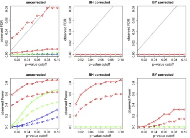
Figure 6 presents the observed FDR and power using
un-corrected, BH un-corrected, and BY correctedP-values for the
sim-ulations based on modelG. Figure 6, top, shows that, except for
the AIC-based nonparametric CMST, the observed FDRs were
considerably lower than theP-value cutoff, suggesting that
mul-tiple testing adjustment is not necessary for the CMST tests. Furthermore, comparison of the bottom panels shows that the BH and BY adjustments leads to a reduction in power (specially for the BY adjustment) for the joint and parametric tests at the expense of small drop in FDR levels (that were already low without any correction). For the nonparametric tests, on the other hand, BH corrections leads to bigger drops in FDR (spe-cially for the AIC based test) and smaller drops in power. The BY correction appears too conservative even for the
nonpara-metric tests. The results for modelFare similar (Figure S13).
Yeast data analysis and biologically validated predictions
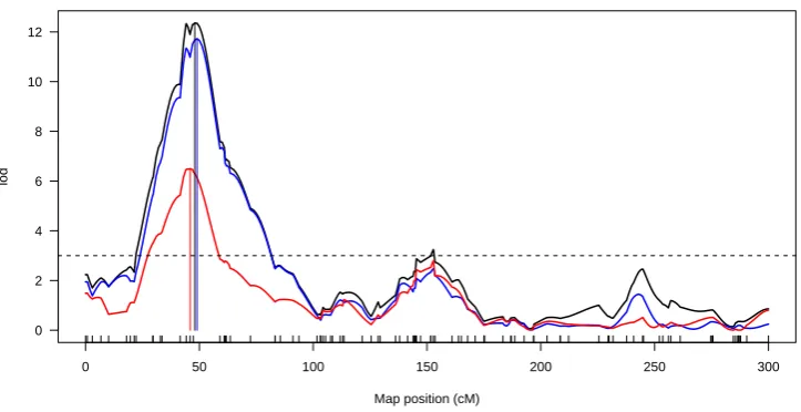
We analyzed a budding yeast genetic genomics data set derived from a cross of a standard laboratory strain and a wild isolate from a California vineyard (Brem and Kruglyak 2005).
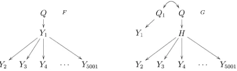
Figure 3 Models generating hotspot patterns.Y1represents acis-expression trait.Yk,k= 2, ..., 5001 represent expression traits mapping intransto the hotspot QTLQ.Hrepresents an unobserved expression trait. ModelF gener-ates a hotspot pattern derived from the causal effect of the master regulator, Y1, on the transcription of the other traits. ModelGgives rise to a hotspot pattern, due to the causal effect ofHonYk, but where thecis-traitY1maps to
Q1, a QTL closely linked to the true QTL hotspotQ, and is actually causally independent of the traits mapping intransto theQ.
Figure 4 Power (A and D), miss-calling error rate (B and E), and precision (C and F) across the simulated models depicted in Fig-ure 2. The x-axis represents the significance levels used for com-puting the results. (A—C) The simulations based on sample size 112; (D—F) the results for sample size 1000. Dashed and solid curves represent, respectively, AIC- and BIC-based methods. Green: parametric CMST. Red: nonparametric CMST. Blue: joint-parametric CMST. Black: AIC and BIC. Orange: CIT. The shaded line on B and E corre-sponds to thealevels.
The data consist of expression measurements on 5740 tran-scripts measured on 112 segregant strains with dense geno-type data on 2956 markers. Processing of the expression measurements raw data was performed as described in Brem and Kruglyak (2005), with an additional step of converting
the processed measurements to normal scores. We performed
QTL analysis using Haley–Knott regression (Haley and Knott
1992) with the R/qtl software (Bromanet al.2003). We used
Haldane’s map function, genotype error rate of 0.0001,
and set the maximum distance between positions at which
Figure 5 Power (A and D), miss-calling error rate (B and E), and precision (C and F) restricted to thecis-vs. trans-cases. Thex-axis represents the significance levels used for computing the results. The results were computed using only the simulated models A, B, D, and E in Figure 2, since the pleiotropic causal relationship depicted in model C is expected to be much less frequent than the others when testingcis-vs. trans-case. (A–C) The simulations based on sample size 112; (D–F) the results for sample size 1000. Dashed and solid curves repre-sent, respectively, AIC- and BIC-based methods. Green: parametric CMST. Red: nonparametric CMST. Blue: joint-parametric CMST. Black: AIC and BIC. Orange: CIT. The shaded line on B and E corre-sponds to thealevels.
Figure 6 Observed FDR and power for the simulations based on model G. The x-axis repre-sents the P-value cutoffs used for computing the results. Dashed and solid curves repre-sent, respectively, AIC- and BIC-based methods. Green: parametric CMST. Red: nonparametric CMST. Blue: joint-parametric CMST. Black: AIC and BIC. The shaded line in the top corresponds to thealevels.
genotype probabilities were calculated to 2 cM. We adopted a permutation LOD threshold (Churchill and Doerge 1994) of 3.48, controlling the genome-wide error rate of falsely
detecting a QTL at a significance level of 5%.
To evaluate the precision of the causal predictions made by the methods we used validated causal relationships extracted from a database of 247 knock-out experiments
in yeast (Hughes et al.2000; Zhu et al.2008). In each of
these experiments, one gene was knocked out, and the ex-pression levels of the remainder genes in control and knocked-out strains were interrogated for differential ex-pression. The set of differentially expressed genes form the knock-out signature (ko-signature) of the knocked-out gene (ko-gene) and show direct evidence of a causal effect of the ko-gene on the ko-signature genes. The yeast data cross and knocked-out data analyzed in this section are available in
the R/qtlyeast package at GITHUB (https://github.com/
byandell/qtlyeast).
To use this information, we: (i) determined which of the
247 ko-genes also showed a significant eQTL in our data set;
(ii) for each one of the ko-genes showing significant
linkages, we determined which other genes in our data set also co-mapped to the same QTL of the ko-gene, generating, in this way, a list of putative targets of the ko-gene; (iii) for each of the ko-gene/putative targets list, we
applied all methods using the ko-gene as theY1phenotype,
the putative target genes as theY2phenotypes, and the
ko-gene QTL as the causal anchor; (iv) for the AIC- and
BIC-based nonparametric CMST tests we adjusted theP-values
according to the Benjamini and Hochberg FDR control
pro-cedure; and (v) for each method we determined the “
vali-dated precision,”computed as the ratio of true positives by
the sum of true and false positives, where a true positive is
defined as an inferred causal relationship where the target
gene belongs to the ko-signature of the ko-gene, and a false positive is given by an inferred causal relation where the target gene does not belong to the ko-signature.
In total 135 of the ko-genes showed a significant QTL,
generating 135 putative target lists. A gene belonged to the putative target list of a ko-gene when its 1.5 LOD support interval (Lander and Botstein 1989; Dupuis and Siegmund
1999; Manichaikulet al.2006) contained the location of the
ko-gene QTL. The number of genes in each of the putative target lists varied from list to list, but in total we tested
31,975“ko-gene/putative target gene”relationships.
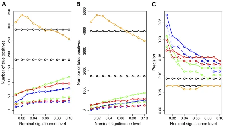
Figure 7 presents the number of inferred true positives, number of inferred false positives, and the prediction
pre-cision across varying target significance levels for each one
of the methods. The CIT, BIC, and AIC had a higher number of true positives than the CMST approaches, with the AIC-based CMST methods having less power than the BIC-AIC-based CMST methods. However, the CIT, BIC, and AIC also inferred the highest numbers of false positives (Figure 7B) and showed low prediction precisions (Figure 7C). From Figure 7C we see that the CMST tests show substantially
higher precision rates across all target significance levels
compared to the AIC, BIC, and CIT methods. Among the CMST approaches, the joint-parametric CMST tended to show the highest precision, followed by the nonparametric and parametric CMST tests.
The results presented in Figure 7 were computed using all 135 ko-genes. However, in light of our simulation results,
which suggest that the analysis ofcis- againsttrans-genes is
usually easier than the analysis oftrans- againsttrans-genes,
we investigated the results restricting ourselves to ko-genes
with significantcis-QTL. Only 28 of the 135 ko-genes were
cis-traits, but, nonetheless, were responsible for 2947 of the
total 31,975 “ko-gene/putative target gene” relationships.
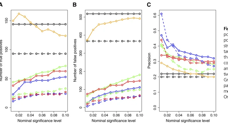
Figure 8 presents the results restricted to the cis-ko-genes.
All methods show improvement in precision, corroborating our simulation results. Once again, the CMST tests showed higher precision than the CIT, AIC, and BIC.
Discussion
In this article, we proposed three novel hypothesis tests that
adapt and extend Vuong’s and Clarke’s model selection tests
to the comparison of four models, spanning the full range of possible causal relationships among a pair of phenotypes. Our CMST tests scale well to large genome wide analyses because they are fully analytical and avoid computationally expensive permutation or resampling strategies.
Another useful property of the CMST tests, inherited
from Vuong’s test, is their ability to perform model selection
among misspecified models. That is, the correct model need
not be one of the models under consideration. Accounting
for the misspecification of the models is key. In general, any
two phenotypes of interest are embedded in a complex net-work and are affected by many other phenotypes not
con-sidered in the grossly simplified (and thus misspecified)
pairwise models.
Overall, our simulations and real data analysis show that the CMST tests are better at controlling miss-calling error rates and tend to outperform the AIC, BIC, and CIT methods in terms of statistical precision. However, they do so at the expense of a decrease in statistical power. While an ideal method would have high precision and power, in practice there is always a trade-off between these quantities. Whether a more powerful and less precise, or a less powerful and more
precise, method is more adequate depends on the biologist’s
research goals and resources. For instance, if the goal is to generate a rank-ordered list of promising candidates genes that might causally affect a phenotype of interest and the bi-ologist can easily validate several genes, a larger list generated by more powered and less precise methods might be more appealing. However, in general, follow-up studies tend to be time consuming and expensive, and only a few candidates can be studied in detail. A long list of putative causal traits is not useful if most are false positives. High power to detect causal relations alone is not enough. A more precise method that
conservatively identifies candidates with high confidence can
be more appealing (see also Chenet al.2007).
Further, the exploratory goal is often to identify causal agents without attempting to reconstruct entire pathways. Therefore, much information about the larger networks in which the tested pairs of traits reside is unknown and generally unknowable and contributes to the large un-explained variation that in turn results in low power. Our
method accurately reflects this difficulty to detect causal
relationships in the presence of noisy high-throughput data and poorly understood networks.
Interestingly, our data analysis and simulations also
suggest that the analysis of cis-against trans-gene pairs is
less prone to detect false positives than the analysis oftrans
-againsttrans-gene pairs. Our simulations suggest that model
selection approaches have difficulty ordering the
pheno-types when the QTL effect reaches the truly reactive gene by two or more distinct paths, only one of which is mediated
by the truly causal gene (seeFigure S1C, for an example).
When we test causal relationships among gene expres-sion phenotypes, the true relationships might not be a direct result of transcriptional regulation. For instance, the true causal regulation might be due to methylation,
phosphory-lation, direct protein–protein interaction, transcription
fac-tor binding, etc. Margolin and Califano (2007) have pointed out the limitations of causal inference at the transcriptional level, where molecular phenotypes at other layers of
regula-tion might represent latent variables. ModelM4(see Figure 1)
can account for these latent variables and can test this sce-nario explicitly.
Furthermore, as pointed out by Li et al. (2010), causal
inference depends on the detection of subtle patterns in the correlation between traits. Hence, it can be challenging even when the true causal relations take place at the transcrip-tional level. The authors point out that reliable causal in-ference in genome-wide linkage and association studies
require large sample sizes and would benefit from: (i)
in-corporating prior information via Bayesian reasoning;
(ii) adjusting for experimental factors, such as sex and age, that might induce correlations not explained the the causal relations; and (iii) considering a richer set of models than the four models accounted in this article.
The CMST tests represent a step in the direction of reliable causal inference in three accounts. First, they tend to be precise, declining to make calls in situations where
alternative approaches usually deliver a flood of
false-positive calls. Second, the CMST tests can adjust for experimental factors by modeling them as additive and interactive covariates. Third, the CMST tests can be applied to nonnested models of different dimensions and can be readily extended to incorporate a larger number of models by implementing intersection-union tests on a larger
num-ber of Vuong’s tests. For the joint-parametric test a
higher-dimensional null distribution is required.
FDR control for the CMST approaches is a challenging problem as our tests violate the key assumption, made by
FDR control procedures, that the distribution of the P
-values under the null hypothesis are uniformly distributed (Benjamini and Hochberg 1995; Storey and Tibshirani
2003). Recall that the CMST P-values are computed as the
maximum across otherP-values, and the maximum of
mul-tiple uniform random variables no longer follows a uniform distribution. Additionally, the CMST tests are usually not
independent since we often test the same cis-trait against
severaltrans-traits, so that the additional assumption of
in-dependent test statistics made by the original Benjamini–
Hochberg procedure does not hold. The Benjamini–Yekutieli
(BY) procedure relaxes the independent test statistics as-sumption, and we explore both these corrections in our sim-ulations. Our results suggest that BH and BY multiple testing correction should not be performed for the joint and the para-metric CMST tests, as the FDR levels are lower than the nom-inal level without any correction and are too conservative with severe reduction in statistical power with the application of
Figure 7 Overall number of true positives (A), number of false positives (B), and precision (C) across all 135 ko-gene/putative target lists. Thex-axis represents the significance levels used for computing the results. Dashed and solid curves represent, re-spectively, AIC- and BIC-based methods. Green: parametric CMST. Red: nonparametric CMST. Blue: joint-parametric CMST. Black: AIC and BIC. Orange: CIT.
BH and BY control. The nonparametric CMST tests, on the
other hand, seemed to benefit from BH correction, showing
slight decrease in power with concomitant decrease in FDR, in spite of the nonparametric CMST tests being based on discrete test statistics and the BH procedure being
devel-oped to handle P-values from continuous statistics.
Inspec-tion of theP-value distributions (seeFigure S14,Figure S15,
Figure S16, and Figure S17) suggests that the smaller
P-values of the nonparametric tests, relative to the other
approaches, are the reason for the higher power achieved by the BH corrected nonparametric tests. The BY procedure, on the other hand, tended to be too conservative even for the nonparametric CMST tests.
The CMST approach is currently implemented for inbred line crosses. Extension to outbred populations involving mixed effects models is yet to be done. Although in this article we focused on mRNA expression traits, the CMST tests can be applied to any sort of heritable phenotype, including clinical
phenotypes and other“omic”molecular phenotypes.
The higher statistical precision and computational effi
-ciency achieved by our fully analytical hypothesis tests will help biologists to perform large-scale screening of causal relations, providing a conservative rank-ordered list of promising candidate genes for further investigations.
Acknowledgments
We thank Adam Margolin for helpful discussions and com-ments and the editor and referees for comcom-ments and suggestions that considerably improved this work.This work was supported by CNPq Brazil (E.C.N.); National Cancer Institute (NCI) Integrative Cancer Biology Program grant U54-CA149237 and National Institutes of Health (NIH) grant R01MH090948 (E.C.N.); National Institute of Diabetes and Digestive and Kidney Diseases (NIDDK) grants DK66369, DK58037, and DK06639 (A.D.A., M.P.K., A.T.B., B.S.Y., E.C.N.); National Institute of
General Medical Sciences (NIGMS) grants PA02110 and GM069430-01A2 (B.S.Y.).
Literature Cited
Akaike, H., 1974 A new look at the statistical model identifi
ca-tion. IEEE Trans. Automat. Contr. 19: 716–723.
Aten, J. E., T. F. Fuller, A. J. Lusis, and S. Horvath, 2008 Using
genetic markers to orient the edges in quantitative trait net-works: the NEO software. BMC Syst. Biol. 2: 34.
Benjamini, Y., and Y. Hochberg, 1995 Controlling the false
dis-covery rate: a practical and powerful approach to multiple
test-ing. J. R. Stat. Soc., B 57: 289–300.
Benjamini, Y., and D. Yekutieli, 2001 The control of the False
Discovery Rate in multiple testing under dependency. Ann. Stat.
29: 1165–1188.
Brem, R., and L. Kruglyak, 2005 The landscape of genetic
com-plexity across 5,700 gene expression trait in yeast. Proc. Natl.
Acad. Sci. USA 102: 1572–1577.
Broman, K., H. Wu, S. Sen, and G. A. Churchill, 2003 R/qtl: QTL
mapping in experimental crosses. Bioinformatics 19: 889–890.
Chaibub Neto, E., C. Ferrara, A. D. Attie, and B. S. Yandell,
2008 Inferring causal phenotype networks from segregating
pop-ulations. Genetics 179: 1089–1100.
Chaibub Neto, E., M. P. Keller, A. D. Attie, and B. S. Yandell,
2010 Causal graphical models in system genetics: a unified
framework for joint inference of causal network and genetic
archi-tecture for correlated phenotypes. Ann. Appl. Stat. 4: 320–339.
Chen, L. S., F. Emmert-Streib, and J. D. Storey, 2007 Harnessing
naturally randomized transcription to infer regulatory relation-ships among genes. Genome Biol. 8: R219.
Churchill, G. A., and R. W. Doerge, 1994 Empirical threshold
values for quantitative trait mapping. Genetics 138: 963–971.
Clarke, K. A., 2007 A simple distribution-free test for nonnested
model selection. Polit. Anal. 15: 347–363.
Duarte, C. W., and Z. B. Zeng, 2011 High-confidence discovery of
genetic network regulators in expression quantitative trait loci
data. Genetics 187: 955–964.
Dupuis, J., and D. Siegmund, 1999 Statistical methods for
map-ping quantitative trait loci from a dense set of markers. Genetics
151: 373–386.
Figure 8 Overall number of true positives (A), number of false positives (B), and precision (C) re-stricted to 28cisko-gene/putative target lists. The x-axis represents the significance levels used for computing the results. Dashed and solid curves represent, respec-tively, AIC- and BIC-based methods. Green: parametric CMST. Red: non-parametric CMST. Blue: joint-para-metric CMST. Black: AIC and BIC. Orange: CIT.
Hageman, R. S., M. S. Leduc, R. Korstanje, B. Paigen, and G. A.
Churchill, 2011 A Bayesian framework for inference of the
genotype-phenotype map for segregating populations. Genetics
181: 1163–1170.
Haley, C., and S. Knott, 1992 A simple regression method for
mapping quantitative trait loci in line crosses using flanking
markers. Heredity 69: 315–324.
Hughes, T. R., M. J. Marton, A. R. Jones, C. J. Roberts, R. Stoughton
et al., 2000 Functional discovery via a compendium of
expres-sion profiles. Cell 102: 109–116.
Kullback, S., 1959 Information Theory and Statistics.Wiley, New York.
Kulp, D. C., and M. Jagalur, 2006 Causal inference of
regulator-target pairs by gene mapping of expression phenotypes. BMC Genomics 7: 125.
Lander, E. S., and D. Botstein, 1989 Mapping Mendelian factors
underlying quantitative traits using RFLP linkage maps.
Genet-ics 121: 185–199.
Li, R., S. W. Tsaih, K. Shockley, I. M. Stylianou, J. Wergedalet al.,
2006 Structural model analysis of multiple quantitative traits.
PLoS Genet. 2: e114.
Li, Y., B. M. Tesson, G. A. Churchill, and R. C. Jansen,
2010 Critical preconditions for causal inference in
genome-wide association studies. Trends Genet. 26: 493–498.
Liu, B., A. de la Fuente, and I. Hoeschele, 2008 Gene network
inference via structural equation modeling in genetical
ge-nomics experiments. Genetics 178: 1763–1776.
Manichaikul, A., J. Dupuis, S. Sen, and K. W. Broman, 2006 Poor
performance of bootstrap confidence intervals for the location of
a quantitative trait locus. Genetics 174: 481–489.
Margolin, A., and A. Califano, 2007 Theory and limitations of
genetic network inference from microarray data. Ann. N.Y.
Acad. Sci. 1115: 51–72.
Millstein, J., B. Zhang, J. Zhu, and E. E. Schadt, 2009 Disentangling
molecular relationships with a causal inference test. BMC Genet.
10: 23 .10.1186/1471–2156–10–23.
Sawa, T., 1978 Information criteria for discriminating among
al-ternative regression models. Econometrica 46: 1273–1291.
Schadt, E. E., J. Lamb, X. Yang, J. Zhu, S. Edwards et al.,
2005 An integrative genomics approach to infer causal
asso-ciations between gene expression and disease. Nat. Genet. 37:
710–717.
Schwarz, G. E., 1978 Estimating the dimension of a model. Ann.
Stat. 6: 461–464.
Shao, J., 2003 Mathematical Statistics,Springer Texts in Statistics,
Ed. 2. Springer, New York.
Storey, J., and R. Tibshirani, 2003 Statistical significance for
ge-nomewide studies. Proc. Natl. Acad. Sci. USA 100: 9440–9445.
Sun, W., T. Yu, and K. C. Li, 2007 Detection of eQTL modules
mediated by activity levels of transcription factors.
Bioinfor-matics 23: 2290–2297.
Vuong, Q. H., 1989 Likelihood ratio tests for model selection and
non-nested hypothesis. Econometrica 57: 307–333.
West, M. A. L., K. Kim, D. J. Kliebenstein, H. van Leeuwen, R. W.
Michelmore et al., 2007 Global eQTL mapping reveals the
complex genetic architecture of transcript-level variation in
Ara-bidopsis. Genetics 175: 1441–1450.
Winrow, C. J., D. L. Williams, A. Kasarskis, J. Millstein, A. D.
Laposkyet al., 2009 Uncovering the genetic landscape for
mul-tiple sleep-wake traits. PLoS ONE 4: e5161.
Zhu, J., P. Y. Lum, J. Lamb, D. GuhaThakurta, S. W. Edwardset al.,
2004 An integrative genomics approach to the reconstruction
of gene networks in segregating populations. Cytogenet. Genome
Res. 105: 363–374.
Zhu, J., M. C. Wiener, C. Zhang, A. Fridman, E. Minch et al.,
2007 Increasing the power to detect causal associations by
combining genotypic and expression data in segregating popu-lations. PLOS Comput. Biol. 3(4): e69 .10.1371/journal. pcbi.0030069.
Zhu, J., B. Zhang, E. N. Smith, B. Drees, R. B. Brem et al.,
2008 Integrating large-scale functional genomic data to
dis-sect the complexity of yeast regulatory networks. Nat. Genet.
40: 854–861.
Communicating editor: L. M. McIntyre
GENETICS
Supporting Information http://www.genetics.org/lookup/suppl/doi:10.1534/genetics.112.147124/-/DC1
Modeling Causality for Pairs of Phenotypes
in System Genetics
Elias Chaibub Neto, Aimee T. Broman, Mark P. Keller, Alan D. Attie, Bin Zhang, Jun Zhu, and Brian S. Yandell
(a)
Q
(b)
Q
(c)
Q
(d)
Q
>>>
> (e)
Q
??? ?
Y
1 } }|||| AAAA
Y
3Y
3 ~ ~|||| AAAA
Y
3Y
4Y
3 ~ ~ ||||Y
4Y
3 ! ! B B BB
Y
4~ ~ }}}}
Y
1Y
1 B B BB
Y
4
Y
1Y
5
Y
1Y
5
Y
5 A A AA
Y
4> > | | | | B B B
B
Y
6
Y
2Y
2Y
6~
~
}}}}
Y
2Y
5
Y
7 v v nnnnnnnnnn
Y
6O O 6 6 n n n n n n n n n n
Y
2Y
2(a′)
Q
~
~
}}}}}
(b′)
Q
~
~
~~~~
(c′)
Q
~
~
~~~~~ ???
? (d′)
Q
>>>
> (e′)
Q
~
~
~~~~~ ???
?
Y
1 //Y
2Y
1 //Y
2Y
1 //Y
2Y
1Y
2Y
1Y
2H
a
a
CCCC ||>>
| |
H
a
a
CCCC ||>>
| |
Figure S 1
Network models and their collapsed versions. The collapsed networks
(bottom panels) represent simplified versions of the true networks (top panels), where
nodes other than
Q
,
Y
1and
Y
2are ignored, even though they still represent the correct
causal flow among these three nodes in the true network. Consider, for example,
network
c
and its collapsed version
c
′. The path
Q
→
Y
3→
Y
1in
c
is collapsed to
Q
→
Y
1in
c
′. The paths
Y
1→
Y
5→
Y
2and
Y
1→
Y
6→
Y
2in
c
are collapsed to
Y
1→
Y
2in
c
′. The path
Q
→
Y
3→
Y
4→
Y
7→
Y
2in
c
is collapsed to
Q
→
Y
2in
c
′.
0.2 0.4 0.6 0.8 0.2
0.4 0.6 0.8 −2
0 2 4 6
R2(Y1, X) R2(Y2, X)
Z12
0.2 0.4 0.6 0.8 0.2
0.4 0.6 0.8 −2
0 2 4 6
R2(Y1, X) R2(Y2, X)
Z12
0.0 0.2 0.4 0.6 0.8
0.0
0.2
0.4
0.6
0.8
R2(Y1, X)
R
2( Y2
,
X
)
0.0 0.2 0.4 0.6 0.8
0.0
0.2
0.4
0.6
0.8
R2(Y1, X)
R
2( Y2
,
X
)
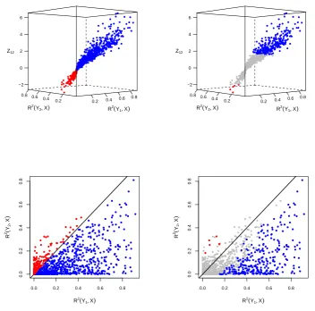
Figure S2
Model selection via log-likelihood ratio versus Vuong’s test.
Figure S2 illustrates how Vuong’s test works. We generated 1,000 data-sets from the
model
X
→
Y
1→
Y
2and applied Vuong’s test to the comparison of models
M
1:
X
→
Y
1→
Y
2against
M
2:
X
→
Y
2→
Y
1. The top panels present 3D scatter plots of the test
statistics
Z
12against the
R
2values of the regression of
Y
1on
X
,
R
2(
Y
1, X
), and the
R
2values of the regression of
Y
2on
X
,
R
2(
Y
2, X
). The data points are color coded as blue,
red and grey, representing, respectively,
M
1,
M
2and “no calls”. Note that because model
M
1corresponds to the true model, we have that the a
M
1call is always correct, whereas
a
M
2call is always incorrect in this example. Therefore, blue and red points represent,
respectively, correct and incorrect calls. The bottom panels follow the same color coding
and show the projections of the 3D scatter plots into the
R
2(
Y
1
, X
) by
R
2(
Y
2, X
) plane.
The left panels of Figure S2 show the model selection results based on the log-likelihood
ratio (LR) criterium, where positive
L
R
ˆ
12values support
M
1and negative
L
R
ˆ
12values
support
M
2(note that we actually use the
Z
12test statistics, instead of
L
R
ˆ
12statistics,
but the results are equivalent). Because we generate the data from model
X
→
Y
1→
Y
2,
it will usually be the case that
X
explains a greater proportion of the variability of
Y
1than of
Y
2. In other words,
R
2(
Y
1, X
) will tend to be higher than
R
2(
Y
2, X
). However,
some of the data-sets show the opposite trend due to random noise on the data. The
bottom left panel shows that the log-likelihood criterium tends to make incorrect calls
when
R
2(
Y
1
, X
)
< R
2(
Y
2, X
).
The right panels of Figure S2 show the model selection results derived from Vuong’s
test. Now we see that most of the incorrect calls made by the log-likelihood criterium
(red points) are not significant (grey points) according to Vuong’s test, that requires that
Z
12≤ −
1
.
64 or
Z
12≥
1
.
64 for statistical significance at a 5% level. The drawback is the
reduction in power to detect the correct calls, since not only red dots are replaced by grey
dots, but many of the blue dots are turned into grey, as well. These figures illustrate how
Vuong’s test trade an increase in precision for a reduction in statistical power to detect
true positives.
File S1
A technical note on Vuong’s test
Vuong (1989) fully characterized the asymptotic distribution of the log-likelihood ratio
statistic under the most general conditions. He showed that the form of the asymptotic
distribution of the log-likelihood ratio depends on whether the models are observationally
identical or not. Two models are observationally identical if their probability densities
are the same, when evaluated at the respective pseudo-true parameter values, i.e.,
f
1(
y
|
x
;
θ
1∗) =
f
2(
y
|
x
;
θ
2∗) for almost all (
y
,
x
), where the pseudo-true parameter values,
θ
k∗, corresponds to the parameter value that minimizes the Kullback-Leibler distance
from the true model (Sawa 1978).
Explicitly, Vuong showed (Theorem 3.3 on page 313) that under very general
condi-tions:
1. If
f
1(
y
|
x
;
θ
1∗) =
f
2(
y
|
x
;
θ
2∗), then 2
LR
12(ˆ
θ
1,
θ
ˆ
2) converges in distribution to a
weighted sum of chi-square distributions.
2. If
f
1(
y
|
x
;
θ
1∗)
̸
=
f
2(
y
|
x
;
θ
2∗), then
1
√
n
(
LR
12(ˆ
θ
1,
θ
ˆ
2)
−
E
0[
log
f
1(
y
|
x
;
θ
1∗)
f
2(
y
|
x
;
θ
2∗)
])
→
dN
(0
, σ
12.12
)
Because of this interesting asymptotic behavior Vuong had to proposed 3 distinct
model selection tests: one for strictly non-nested models, that are always not
observation-ally identical; another for overlapping models that might or might not be observationobservation-ally
identical; and a third for nested models, that are always observationally identical. (Nested
models are always observationally identical because the nested model cannot be better
than the full model and both models are equally close to the true model if and only if
they are the same.)
In our applications, models
M
1,
M
2and
M
3are not nested on each other, but are
nested on models
M
a4