Unbiased Estimation of Gene Diversity in Samples Containing Related Individuals: Exact Variance and Arbitrary Ploidy

DOI: 10.1534/genetics.110.121756

Unbiased Estimation of Gene Diversity in Samples Containing Related

Individuals: Exact Variance and Arbitrary Ploidy

Michael DeGiorgio,*

,1,2

_{Ivana Jankovic*}

,1,3

_{and Noah A. Rosenberg*}

,†

*Center for Computational Medicine and Bioinformatics, University of Michigan, Ann Arbor, Michigan 48109 and†Department of Human Genetics and the Life Sciences Institute, University of Michigan, Ann Arbor, Michigan 48109

Manuscript received August 3, 2010 Accepted for publication September 21, 2010

ABSTRACT

Gene diversity, a commonly used measure of genetic variation, evaluates the proportion of heterozy-gous individuals expected at a locus in a population, under the assumption of Hardy–Weinberg equilibrium. When using the standard estimator of gene diversity, the inclusion of related or inbred individuals in a sample produces a downward bias. Here, we extend a recently developed estimator shown to be unbiased in a diploid autosomal sample that includes known related or inbred individuals to the general case of arbitrary ploidy. We derive an exact formula for the variance of the new estimator,H, and˜ present an approximation to facilitate evaluation of the variance when each individual is related to at most one other individual in a sample. When examining samples from the human X chromosome, which represent a mixture of haploid and diploid individuals, we find thatH˜ performs favorably compared to the standard estimator, both in theoretical computations of mean squared error and in data analysis. We thus propose that H˜ is a useful tool in characterizing gene diversity in samples of arbitrary ploidy that contain related or inbred individuals.

F

OR a given locus, gene diversity, also known as expected heterozygosity, characterizes the propor-tion of heterozygous genotypes expected in a populapropor-tion under Hardy–Weinberg equilibrium (Nei 1973). Nei

and Roychoudhury (1974) devised an estimator of

gene diversity that is unbiased for random samples of unrelated, noninbred individuals. When inbred individ-uals or close relatives are included in a sample, how-ever, this estimator has a downward bias (Weir 1989;

DeGiorgioand Rosenberg2009). To account for the

effects of inbreeding in a sample of diploid individuals, Weir(1989, 1996) derived the expected value of gene

diversity, producing an unbiased estimator of gene diversity that makes use of the mean inbreeding coeffi-cient across sampled individuals, where the inbreeding coefficient of an individual is defined as the probability for a randomly chosen locus that the two alleles of the individual are inherited identically by descent from a common ancestor. Using the mean kinship coefficient across pairs of sampled individuals, DeGiorgio and

Rosenberg(2009) extended this estimator to account

for the bias produced in samples containing close relatives, where the kinship coefficient between two

individuals, j and k, is defined as the probability that an allele randomly selected from individualj at a ran-dom locus and an allele ranran-domly selected from indi-vidualkat the same locus are identical by descent (IBD). The DeGiorgioand Rosenberg(2009) estimator is

useful for autosomal markers in samples from diploid organisms that contain related or inbred individuals. However, in studying gene diversity among related individuals in nondiploid cases (e.g., Buteler et al.

1999) or in cases of mixed ploidy, such as in the analysis of sex chromosomes (e.g., Reiland et al. 2002),

unbi-asedness for this estimator has not been demonstrated. Here, we extend the DeGiorgioand Rosenberg(2009)

estimator of gene diversity to account for situations in which known related and inbred individuals are in-cluded in a sample and in which the sample contains an arbitrary mixture of individuals of different ploidy. We use a more general method to obtain the estimator than the method used for diploids by DeGiorgio and

Rosenberg (2009), and we show that the general

esti-mator reduces to the DeGiorgio and Rosenberg

(2009) estimator in the diploid case. We also derive a formula for the variance of our estimator,H, to facilitate˜ evaluation of the statistical properties of the estimator. This variance formula, which is a function of identity states among individuals, includes terms that involve identity-by-descent among two, three, and four individ-uals and among pairs of pairs of individindivid-uals. Our variance function is convenient because extensive work on IBD probabilities among individuals (e.g., Cotterman 1_{These authors contributed equally to this work.}

2_{Corresponding author: Center for Computational Medicine and}

Bio-informatics, University of Michigan, 2017 Palmer Commons, 100 Washtenaw Ave., Ann Arbor, MI 48109-2218.

E-mail: [email protected]

3_{Present address: David Geffen School of Medicine, University of}

California, Los Angeles, CA 90095.

1940; Harris 1964; Gillois 1965; Cockerham 1971;

Jacquard1974; Thompson1974; Lange2002) has

pro-vided a framework for calculating the quantities incorpo-rated in the formula.

Using the variance formula, we examine the perfor-mance of our estimator in scenarios involving the human X chromosome, for which males and females, who might both be included in a typical sample, differ in ploidy. In our evaluations, we first show that the exact theoretical values of the variance, which are obtained from a quite complex formula, are closely matched by simulations. We also validate that when each sampled individual is related to at most one other individual in the sample, the exact theoretical variance can be approximated well by a simpler formula. Using the variance approximation and simulations, we compare the behavior of our esti-mator to that of the Nei and Roychoudhury (1974)

estimator, which does not account for relatives. We then analyze human SNPs from the X chromosome and find thatH˜also performs well in practice.

THEORY

Consider a sample of ggroups, each with different ploidy (e.g., haploid males and diploid females on the human X chromosome). Suppose that the sample from groupbcontainsnbmb-ploid individuals,b¼1, 2,. . .,g. Further, let (b,k),k¼1, 2,. . .,nb, denote individualk from groupb. The number of copies of allelic typeiin individualkfrom groupbis

Xð_ði_bÞ;kÞ¼

Xmb

‘¼1

Að_ði_bÞ;kÞ;‘; ð1Þ

whereAð Þði_b;kÞ;‘is an indicator random variable that takes on the value 1 if the‘th allele in individual (b,k) has typeiand that equals 0 otherwise.

Note that E½Aðð Þ_bi;kÞ;‘ ¼pi, where pi is the frequency of allelic typeiin the population. We can then define an unbiased estimator for the frequency of alleleias

ˆpi¼

1

Pg b¼1nbmb

Xg

b¼1

Xnb

k¼1

Xð_ði_bÞ_;kÞ: ð2Þ

Rewriting the estimator of Nei and Roychoudhury

(1974) for the mixed-ploidy case, if no inbred or related individuals are included in the sample, then an un-biased estimator of gene diversity is

ˆ H¼

Pg b¼1nbmb ðPg_b¼1nbmbÞ 1

1X I

i¼1 ˆp2

i

!

: ð3Þ

If inbred or related individuals are included in the sam-ple, thenHˆ is a biased estimator of H ¼1PI

i¼1p 2

i. We follow the approach of DeGiorgioand Rosenberg

(2009), correcting for this bias by first obtaining the variance of sample allele frequencies. However, we use

a different method here for obtaining the variance of sample allele frequencies, determining the bias correc-tion for diploids as a special case of a more general computation.

An unbiased estimator: Suppose we have four possi-bly, but not necessarily, distinct individuals (a,j), (b,k), (a9, j9), and (b9, k9). Define F(a,j)(b,k) as the

probabil-ity that two alleles randomly chosen, one from individ-ual (a, j) and the other from individual (b, k), are IBD. Similarly, define F(a,j)(b,k)(a9,j9) as the probability

that three alleles randomly chosen, one from (a, j), one from (b,k), and one from (a9,j9), are IBD. Define F(a,j)(b,k)(a9,j9)(b9,k9) as the probability that four alleles

randomly chosen, one from (a,j), one from (b,k), one from (a9, j9), and one from (b9, k9), are IBD. Finally, define F(a,j)(b,k),(a9,j9)(b9,k9) as the joint probability that

two alleles randomly chosen, one from (a,j) and the other from (b, k), are IBD and two alleles randomly chosen, one from (a9,j9) and the other from (b9,k9), are IBD. These four types of probability of identity-by-descent are identical to theu,g,d, andDcoefficients of Cockerham(1971), respectively. We can then define

F₂¼X g

a¼1

Xg

b¼1

Xna

j¼1

Xnb

k¼1

wawbFða;jÞðb;kÞ ð4Þ

F₃¼X g

a¼1

Xg

b¼1

Xg

a9¼1

Xna

j¼1

Xnb

k¼1

Xna9

j9¼1

wawbwa9Fða;jÞðb;kÞða9;j9Þ ð5Þ

F4¼

Xg

a¼1

Xg

b¼1

Xg

a9¼1

Xg

b9_¼1

Xna

j¼1

Xnb

k¼1

Xna9

j9¼1

Xnb9

k0¼1

wawbwa9wb9Fða;jÞðb;kÞða9;j9Þðb9;k9Þ

ð6Þ

F2;2¼

Xg

a¼1

Xg

b¼1

Xg

a9¼1

Xg

b9_¼1

Xna

j¼1

Xnb

k¼1

Xna9

j9¼1

Xnb9

k9¼1

wawbwa9wb9Fða;jÞðb;kÞ;ða9;j9Þðb9;k9Þ

ð7Þ

as weighted mean kinship coefficients across all sets of pairs, triplets, quartets, and pairs of pairs of individuals. The weight associated with an individual in group x, wx ¼mx=

Pg

b¼1nbmb, is proportional to the ploidy asso-ciated with the group. Define the inbreeding coefficient for individual (b,k), denoted byf(b,k), as the probability

that two alleles randomly chosen without replacement from individual (b, k) are IBD and let fb ¼

1=nb

ð ÞPnb

k¼1fðb;kÞ be the mean inbreeding coefficient

across individuals in groupb. This definition reduces to the standard definition for the diploid case.

and Rosenberg (2009) for diploids to the case of

ar-bitrary ploidy (Equations 13 and 14) and we show how these generalizations can be reduced to the diploid case. Consider a locus withIdistinct alleles, allele frequen-ciespi2[0, 1], andPIi¼1pi ¼1. Suppose a sample from a population hasggroups, each with different ploidy, and nbmb-ploid individuals in groupb,b¼1, 2,. . .,g, each of whom is possibly inbred and related to other individuals in the sample. Consider the‘th allele of individual (a,j) and thetth allele of individual (b, k). By definition of expected value, we have

E _AðiÞ ða;jÞ;‘A

ðiÞ ðb;kÞ;t

h i

¼P AððiaÞ;jÞ;‘¼1;A

ðiÞ ðb;kÞ;t¼1

h i

¼Fða;jÞðb;kÞpi1ð1Fða;jÞðb;kÞÞp2_i ¼Fða;jÞðb;kÞpið1piÞ1 p2i: ð8Þ

In taking the expected value of our estimator of gene diversity, we need to evaluate the quantityE ˆp2

i . Using Equation 8, we show inappendix athat

E _ˆp2

i ¼ F2pið1piÞ1p2i: ð9Þ

Plugging Equations 8 and 9 into Var½ ¼ˆpi E ˆp2i

E_{½ ˆpi}

ð Þ2 yields Var½ ¼ˆpi F2pið1piÞ, which reduces to the result presented for the diploid case in Equation 7 of DeGiorgioand Rosenberg(2009), by reduction of the

definition of F2 for the diploid case. The following

theorem provides a generalized unbiased estimator of gene diversity when a sample with any mixture of ploidy contains related or inbred individuals.

Theorem1.Consider a locus with I distinct alleles,allele

frequencies pi 2[0, 1],and

PI

i¼1pi¼1.Suppose a sample from a population has g groups,each with different ploidy,and nbmb-ploid individuals in group b,b¼1, 2,. . .,g,each of whom is possibly inbred and related to other individuals in the sample. Then

˜ H¼ 1

1F2

1X I

i¼1 ˆp2

i

!

ð10Þ

is an unbiased estimator for gene diversity.

The proof thatH˜ is unbiased follows that of Propo-sition 1 in DeGiorgioand Rosenberg(2009),

substitut-ing the more generalF2in place of the corresponding

mean kinship coefficient in the earlier proof.

When reducing the definition ofF2 for the diploid

case studied by DeGiorgio and Rosenberg (2009),

the result in Theorem 1 is identical to the result pre-sented for this case in Proposition 1 of DeGiorgioand

Rosenberg (2009). One interesting consequence of

Theorem 1 is that H˜ has a simple representation in terms of the sample proportion of identity-by-state and the probability of identity-by-descent computed on the

basis of assumed levels of inbreeding and relationship. This representation is

˜

H¼1ˆP½IBS

1P½IBD; ð11Þ

whereˆP½IBS is the probability that two alleles in the sample, chosen uniformly at random with replacement, are identical by state, andP[IBD] is the probability that two alleles in the sample, chosen uniformly at random with replacement, are identical by descent. A proof that Equation 11 is a consequence of Equation 10 is provided in appendix a. Note that Equations 10 and 11 have a

connection to estimators of relatedness in a context in which relatedness is unknown. Such estimators essen-tially invert equations similar to Equation 11 to get estimators ofF₂(Ritland1996; Rousset2002).

We next seek to transform the estimator in Equation 10 into one that is more convenient for data analysis. Let

Ga,b, a, b ¼ 1, 2,. . ., g, be the set of distinct types of

relative pairs for pairs of distinct individuals in a sample, one from groupaand one from groupb. LethRbe the number of pairs of individuals with relationship typeR inGa,b,and letFRbe the kinship coefficient for each of these pairs. Then, as shown inappendix a, we can write

F2as

F2¼

1

ðPg_b¼1nbmbÞ2

3 X g

b¼1

nbmb1

Xg

b¼1

nbmbðmb1Þfb12

Xg

b¼1

X

R2Gb;b m2bhRFR

2 4

12X

g1

a¼1

Xg

b¼a11

X

R2Ga;b

mambhRFR

3

5:

ð12Þ

This version of F2 is convenient for computation. To

obtain a formula forH˜ that is convenient for computa-tion and that is a generalized version of an analo-gous quantity for the diploid case in Equation 9 of DeGiorgioand Rosenberg(2009), we can substitute

Equations 3 and 12 into Equation 10 to get

˜ H¼ð

Pg

b¼1nbmbÞðPbg¼1nbmb1Þ

D Hˆ; ð13Þ where

D¼ X g

b¼1 nbmb

! Xg

b¼1

nbmb1

!

X

g

b¼1

nbmbðmb1Þfb

2X

g

b¼1

X

R2Gb;b

m2_bh_RF_R2X

g1

a¼1

Xg

b¼a11

X

R2Ga;b

mambhRFR:

A proof of Equation 13 is provided inappendix a. We

note that by usingg¼1,n1¼n, andm1¼2 in Equation 13,

we obtain Equation 9 of DeGiorgioand Rosenberg

Note thatH˜ ¼c ˆH, where

c ¼ð

Pg

b¼1nbmbÞðPbg¼1nbmb1Þ

D :

By rearranging and taking the expected value, we get

E_Hˆ _¼E_{½ H}˜ =c¼H=c. Therefore,

biasð_Hˆ_{Þ ¼}1c c H

¼ 1

ðPg_b¼1nbmbÞðPgb¼1nbmb1Þ

3 X

g

b¼1

nbmbðmb1Þfb12

Xg

b¼1

X

R2Gb;b

m2_bhRFR

2 4

12X

g1

a¼1

Xg

b¼a11

X

R2Ga;b

mambhRFR

3 5H:

ð14Þ

Equation 14 is a generalized version of the bias formula in the diploid case, in Equation 11 of DeGiorgioand

Rosenberg (2009). The bias is always negative and it

has a magnitude that increases linearly with respect to H. Usingg¼1,n1¼n, andm1¼2 in Equation 14, we

obtain Equation 11 of DeGiorgio and Rosenberg

(2009).

Variance of the estimator: In the previous section, we derived an unbiased estimator_H˜ of gene diversity in a sample of arbitrary ploidy. It is useful to determine the variance of the estimator, a quantity that in the diploid case DeGiorgio and Rosenberg (2009)

ob-tained only by simulation. The following theorem provides a formula for the variance of the generalized estimator of gene diversity in samples with any mixture of ploidy.

Theorem2.Consider a locus with I distinct alleles,allele

frequencies pi2 [0, 1],and PIi¼1pi¼1.Suppose a sample from a population has g groups,each with different ploidy,and nbmb-ploid individuals in group b,b¼1, 2,. . .,g,each of whom is possibly inbred and related to other individuals in the sample. Then the variances of the ˜H and ˆH estimators of gene diversity are

Var½ ¼H˜ 1

ð1F₂Þ2Var 1

XI

i¼1 ˆp2

i

" #

ð15Þ

and

VarHˆ ¼

Pg b¼1nbmb ðPg_b¼1nbmbÞ 1

" #2

Var 1X I

i¼1 ˆp2

i

" #

; ð16Þ

where

Var 1X I

i¼1 ˆp2

i

" #

¼F_2;2F2

212 F22F4

XI

i¼1 p2_i

14 2F41F22F3F2;2

XI

i¼1 p3_i

1 3F_2;218F₃6F₄4F₂F2₂

_XI

i¼1 p2_i

!2 :

ð17Þ

The proof of Theorem 2 is long and is provided in

appendix b.

We next derive an approximate formula that in our calculations below we use in place of Equation 17 inside of Equations 15 and 16. The approximation is based only on pairwise kinship coefficients and is useful in cases in which the number of relatives in a sample is small enough that no individual is related to more than one other sampled individual. In such cases, the only nonzero terms included inF3,F4, andF2;2all involve sampling the same

individual or pairs of individuals more than once. Thus, theF3,F4, andF2;2terms, along withF22, are ignored, as

they are likely to be much smaller than F2 in cases in

which the number of relationships in the sample is small. In addition to the assumptions listed in Theorem 2, suppose that each individual in the sample is related to no more than one other individual in the sample. If we ignore terms involvingðPgb¼1mbnbÞ

k

,k.1, then terms involving F2

2,F3,F4, andF2;2in Equation 17 can be ignored. The

only terms in Equation 17 that we retain are those of order_P g

b¼1mbnb

ð Þ0

and ðPgb¼1mbnbÞ

1

. F2 is of order

Pg b¼1mbnb

ð Þ1

. Therefore, reducing Equation 17 leads to

Var 1X I

i¼1 ˆp2

i

" #

4F₂ X

I

i¼1

p3_i X I

i¼1 p2_i

!2

" #

: ð18Þ

This formula is an approximation to Equation 17 when the number of relatives in a sample is small enough that no individual is related to more than one other sampled individual.

We now show that when no related individuals are included in a sample of diploids, the variance in Equation 18 is exactly the formula given by Weir(1989). Suppose a

sample from a diploid population consists ofnunrelated, but possibly inbred, individuals. Further suppose that we ignore terms involvingnk

,k.1. ThenF_kk¼(1/2)(11 fk), wherefkis the inbreeding coefficient for individualk. We can write the mean pairwise kinship coefficient as

F₂¼ 1

n2

Xn

k¼1

F_kk ¼ 1

n2

Xn

k¼1 1

2ð11fkÞ ¼ 1

2nð11fÞ; where f ¼ð1=nÞPn

k¼1fk is the mean inbreeding co-efficient across individuals. PluggingF₂ ¼11f=ð2nÞ

Var 1X I

i¼1 ˆp2

i

" #

2

nð11fÞ

XI

i¼1

p3_i X I

i¼1 p2_i

!2

" #

:

ð19Þ

The X chromosome case: A common situation in which data of mixed ploidy arise is on sex chromo-somes, for which members of one sex have two copies of a specific sex chromosome and members of the other sex have one copy. Later, we examine data on the human X chromosome, for which females have two copies and males have one. Thus, we now utilize Equation 13 to derive an unbiased estimator of gene diversity in samples from the X chromosome.

Consider an X-linked locus with I distinct alleles, allele frequenciespi2[0, 1], and

PI

i¼1pi¼1. Suppose a sample from a population has nF females and nM

males, each of whom is possibly inbred and related to other sampled individuals. LetM,F, andUbe the

sets of distinct types of male–male, female–female, and male–female relative pairs in the sample, respectively. Further, let hR be the number of pairs of individuals with relationship type R and let FR be the kinship coefficient for each of these pairs. Let males be group 1 and let females be group 2. Pluggingg¼2,n1¼nM,

n2¼nF,m1¼1, andm2¼2 into Equation 13, we obtain

an unbiased estimator for gene diversity at an X-linked locus as

˜

H¼ ðnM12nFÞðnM12nF1Þ

ðnM12nFÞðnM12nF1Þ 2nFfF2PR2MhRFR8PR2FhRFR4PR2UhRFR

ˆ H;

ð20Þ

where fF¼ð1=nFÞ

PnF

k¼1fk is the mean inbreeding co-efficient across female individuals andfkis the inbreed-ing coefficient for femalek.

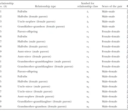
The following special case of Equation 20 is useful for the examples we consider in subsequent sections. It TABLE 1

Relationship types with corresponding X-linked kinship coefficients

Relationship

no. (k) Relationship type

Symbol for

relationship class Sexes of the pair F

1 Full-sibs t1 Male–male 1₂

2 Half-sibs (female parent) t1 Male–male 1₂

3 Uncle–nephew (female parent) t2 Male–male 1₄

4 Grandfather–grandson (female parent) t1 Male–male 1₂

5 Parent–offspring v1 Female–female 1₄

6 Full-sibs v2 Female–female 3₈

7 Half-sibs (male parent) v1 Female–female 1₄

8 Half-sibs (female parent) v3 Female–female 1₈

9 Aunt–niece (male parent) v3 Female–female 1₈

10 Aunt–niece (female parent) v4 Female–female ₁₆3

11 Grandmother–granddaughter (male parent) v1 Female–female 1₄

12 Grandmother–granddaughter (female parent) v3 Female–female 1₈

13 Parent–offspring u1 Male–female 1₂

14 Full-sibs u2 Male–female 1₄

15 Half-sibs (female parent) u2 Male–female 1₄

16 Uncle–niece (male parent) u2 Male–female 1₄

17 Uncle–niece (female parent) u3 Male–female 1₈

18 Aunt–nephew (female parent) u4 Male–female 3₈

19 Grandfather–granddaughter (female parent) u2 Male–female 1₄

20 Grandmother–grandson (female parent) u2 Male–female 1₄

makes use of Table 1, which shows the various types of relationships possible for the X chromosome in pairs of individuals. Suppose a noninbred sample from a pop-ulation hasnFfemales andnMmales, among whichhk pairs of relationship typekare included. LetFkbe the kinship coefficient for each of these pairs. Because the sample is not inbred, the mean inbreeding coefficient across female individuals is fF¼0. Plugging fF as

well ashkandFkfor each relationship typek(Table 1) into Equation 20, we obtain

˜

H¼ ðnM12nFÞðnM12nF1Þ ðnM12nFÞðnM12nF1Þ 2

P4 k¼1hkFk8

P12 k¼5hkFk4

P20 k¼13hkFk

ˆ H:

ð21Þ

DATA ANALYSIS

Data: We investigated the properties ofH˜ on mixed-ploidy data using analytical computations of bias,

variance, and mean squared error; simulations; and analysis of data from human populations. Our choices for simulation parameters were designed on the basis of values in the data. In our analytical computations and simulations, we based our assumed true allele frequen-cies on sample allele frequenfrequen-cies at 36 X-chromosomal loci typed in 950 unrelated individuals, 624 males and 326 females, from the Human Genome Diversity Panel (HGDP-CEPH) microsatellite data set of 1048 individ-uals (Ramachandranet al. 2008). Individuals 127 and

139 from the Ramachandranet al. (2008) data set were

not included in our analyses. The 950 individuals were assumed to have no first- or second-degree relation-ships, on the basis of the Rosenberg(2006) analysis of

the full HGDP-CEPH panel.

Our data analysis was performed on a data set of 13,052 X-chromosomal single-nucleotide polymor-phism (SNP) loci genotyped in 485 individuals from 29 populations in the HGDP-CEPH panel ( Jakobsson

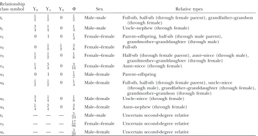
TABLE 2

Symbols used for relative pair types

Relationship

class symbol Y₀ Y₁ Y₂ F Sex Relative types

t1 1₂ 1₂ 0 1₂ Male–male Full-sib, half-sib (through female parent), grandfather–grandson

(through female)

t2 3₄ 1₄ 0 1₄ Male–male Uncle–nephew (through female)

v1 0 1 0 1₄ Female–female Parent–offspring, half-sib (through male parent),

grandmother–granddaughter (through male)

v2 0 1₂ 1₂ 3₈ Female–female Full-sib

v3 1₂ 1₂ 0 1₈ Female–female Half-sib (through female parent), aunt–niece (through male),

grandmother–granddaughter (through female)

v4 1₄ 3₄ 0 ₁₆3 Female–female Aunt–niece (through female)

u1 0 1 0 1₂ Male–female Parent–offspring

u2 1₂ 1₂ 0 1₄ Male–female Full-sib, half-sib (through female parent), uncle–niece

(through male), grandfather–granddaughter (through female), grandmother–grandson (through female)

u3 3₄ 1₄ 0 1₈ Male–female Uncle–niece (through female)

u4 1₄ 3₄ 0 3₈ Male–female Aunt–nephew (through female)

t3 — — — ₂₄5 Male–male Uncertain second-degree relative

v5 — — — 17₉₆ Female–female Uncertain second-degree relative

u5 — — — ₂₀3 Male–female Uncertain second-degree relative

Y0,Y1, andY2designate the probabilities that individuals share 0, 1, and 2 alleles IBD at an X-linked locus, respectively. All types

of relative pairs denoted by the same symbol have the same kinship coefficient, sexes, and probabilities of sharing 0, 1, and 2 alleles IBD.Fcan be calculated fromY1andY2usingFij ¼Y1ifiandjare both male,Fij¼14Y1112Y2 ifiandj are both female,

andFij¼1₂Y11Y2ifiis male andjis female. For each possible pair of sexes (male–male, female–female, and male–female),

the kinship coefficient for second-degree relatives of an uncertain type was found by averaging the kinship coefficients for all second-degree relationships in Table 1 with that pair of sexes, assuming that all were equally likely. Second-degree relationships include half-sib, grandparent–grandchild, and avuncular pairs. For male–male pairs,t3¼ 231₂1131₄1330

=6¼ 5 24. For

female–female pairs, v5¼ 231₄1331₈113₁₆3

=6¼17

96. For male–female pairs, u5¼ 431₄1131₈1133₈1430

= 10¼ 3

20. The divisor in each of the previous equations describes the total number of possible second-degree relatives for that

sex pair (e.g., grandmother–grandson, aunt–nephew, etc., for the male–female case). This number includes second-degree relatives that are not related on the X chromosome, because the assignment of relationships in the data set was based on auto-somal data. The kinship coefficients fort3,v5, andu5were used only for analysis of population data, and they were not used in our

et al. 2008). We also removed individuals related through the X chromosome, yielding a data set of 446 unrelated individuals. Unlike the Jakobsson et al.

(2008) data set of 443 unrelated individuals, our set of 446 individuals did not retain individuals 866, 1046, or 1049, which are not in the H952 subset of the HGDP-CEPH panel. However, individuals 292, 451, 477, 983, 988, and 1089 were included in the data set of non-relatives because they were all involved exclusively in male–male parent–offspring relationships and were therefore unrelated through the X chromosome to other sampled individuals.

Data analysis methods: We used simulations and analytical calculations to evaluate the behavior of the estimatorH˜ for X-chromosomal loci under conditions of varying heterozygosities, sample sizes, and relation-ships of sampled individuals. We compared the relative performance of H˜ and Hˆ by applying H˜ and Hˆ to samples containing related individuals and Hˆ to sam-ples in which relatives were removed so that no relative pairs remained. True allele frequencies were based on microsatellite sample allele frequencies (seeData). In the simulations, individuals of a relative pair were generated by randomly choosing the allele(s) of the first individual on the basis of the empirical allele frequency distribution from the data set. For a given type of relative pair, we then simulated the allele(s) of the second individual by copying alleles from the first individual using the probabilities of sharing zero, one,

and two alleles IBD for that type of pair. Table 2 depicts these probabilities, as well as the symbols used here to denote the various classes of relative pairs. If only one allele was shared, then it was copied in the second individual from the first allele of the first (indepen-dently generated) individual. In cases of male–female relative pairs, the male was generated first and the second allele of the female was always chosen indepen-dently from the allele frequency distribution.

To create a reduced data set of unrelated individuals, the second (possibly dependent) individual was not included for same-sex pairs, whereas for male–female pairs, the male relative was removed. Thus, because each individual in our simulation was included in exactly one relative pair, the number of individuals used to calculate Hˆ for the unrelated sample was al-ways half of that used for the other two estimators. Removing the male in male–female pairs results in the loss of one-third of the alleles, compared to a loss of one-half of the alleles for removal of an individual from a same-sex pair. Thus, compared to removing females, removing males from male–female pairs gen-erates a larger sample of alleles while still ensuring that no individuals are related.

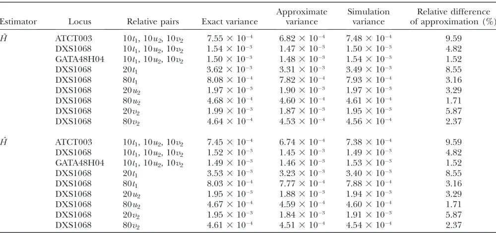
The value assumed for the true heterozygosity,H, of a specific locus, was calculated from the assumed true allele frequencies on the basis of genotypic data of the 950 unrelated individuals. In each simulated scenario, for each of the three estimators, this true heterozygosity TABLE 3

Comparison of exact, approximate, and simulation variances

Estimator Locus Relative pairs Exact variance

Approximate variance

Simulation variance

Relative difference of approximation (%)

˜

H ATCT003 10t1, 10u2, 10v2 7.553104 6.823104 7.483104 9.59

DXS1068 10t1, 10u2, 10v2 1.543103 1.473103 1.503103 4.82

GATA48H04 10t1, 10u2, 10v2 1.503103 1.483103 1.543103 1.52

DXS1068 20t1 3.623103 3.313103 3.493103 8.55

DXS1068 80t1 8.083104 7.823104 7.933104 3.16

DXS1068 20u2 1.973103 1.903103 1.973103 3.29

DXS1068 80u2 4.683104 4.603104 4.613104 1.71

DXS1068 20v2 1.993103 1.873103 1.953103 5.87

DXS1068 80v2 4.643104 4.533104 4.563104 2.37

ˆ

H ATCT003 10t1, 10u2, 10v2 7.453104 6.743104 7.383104 9.59

DXS1068 10t1, 10u2, 10v2 1.523103 1.453103 1.493103 4.82

GATA48H04 10t1, 10u2, 10v2 1.493103 1.463103 1.533103 1.52

DXS1068 20t1 3.533103 3.233103 3.403103 8.55

DXS1068 80t1 8.033104 7.773104 7.883104 3.16

DXS1068 20u2 1.953103 1.883103 1.943103 3.29

DXS1068 80u2 4.673104 4.593104 4.603104 1.71

DXS1068 20v2 1.953103 1.843103 1.913103 5.87

DXS1068 80v2 4.613104 4.513104 4.543104 2.37

The exact (Equations 15 and 16), approximate (Equation 18 inserted into Equations 15 and 16), and simulation variances were calculated for the combination of 10 male–male (t1), 10 male–female (u2), and 10 female–female (v2) full-sib pairs at the

was compared to the mean of the estimates produced by the estimator in 100,000 replicate simulations. The subscript full is used to denote cases in which an estimator was applied to the entire sample, whereas the subscript reduced indicates that relatives were re-moved from the sample. For a given scenario, the bias of each estimator was found by subtracting H from the mean value of the estimates for that estimator. Variance was calculated as the squared mean of the estimates across simulations subtracted from the mean across simulations of the squares of the estimates. Mean squared error (MSE) was then calculated as the sum of bias squared and variance.

Approximate variance:Because each of our analyses was performed on samples that contained only pairs of related individuals, the assumptions that underlie the derivation of the approximate variance (Equation 18) apply. We compared the exact, the approximate, and the simulated variance forH˜ andHˆ in a series of cases that included only full-sib pairs. We chose nine representative cases of the various parameters that can affect estimator performance. Three of these cases considered an equal

mix of male–male, female–female, and male–female full-sib pairs at the ATCT003 (H¼0.7794), DXS1068 (H¼

0.7344), and GATA48H04 (H¼0.6476) loci, chosen to represent high, intermediate, and low heterozygosity, respectively. Additionally, we considered cases at the intermediate-heterozygosity locus involving 20 male– male, 80 male–male, 20 female–female, 80 female– female, 20 male–female, and 80 male–female pairs, to examine the effects of sample size and the sexes of the individuals. In each of our evaluations, we calculated the exact variances (Equations 15 and 16), approximate variances (Equation 18 plugged into Equations 15 and 16), and simulation variances obtained from 100,000 replicate simulations.

As Table 3 shows, in all cases examined, the exact, approximate, and simulated variances are similar, with the approximate variance slightly underestimating the exact variance. Because of the complexity of the formula for the exact variance, the difference between the approximate variance and the exact variance does not have a simple dependence on heterozygosity or sample size. However, it can be observed in Table 3 that for both

Figure1.—Mean squared error, variance, and bias squared for each estimator, obtained analytically using the variance

approx-imation (Equation 18 inserted into Equations 15 and 16), as a function of heterozygosity for 36 loci. The scheme considered included 60 individuals in 10t1pairs (F¼1₂), 10u2pairs (F¼1₄), and 10y2pairs (F¼3₈). (A)Hˆfull. The curve through the

˜

HandH, the relative difference between the approxi-ˆ mate variance and exact variances is smallest at low heterozygosity and large sample size, typically near

2%. In cases of high heterozygosity and small sample size, the relative difference remains at most 10%. We note that the same approximation to the variance of 1PI

i¼1ˆp2i in Equation 18 is applied in obtaining the approximate variances of both H˜ and H. Thus,ˆ because the approximation is generally reasonably accurate and because it treats H˜ and Hˆ in the same way, our use of the approximation is sensible in our subsequent comparisons of the mean squared errors ofH˜ andH.ˆ

Effect of parameters on the estimators:Several fac-tors can potentially affect the performance of the estimators. These factors include the true value of het-erozygosity itself, the sample size, the type of relative

pair represented in the sample, and, if multiple types of relative pairs are included, the combination of particu-lar types of relative pairs. We now examine each of these factors in sequence.

Varying heterozygosity: To investigate the influence of varying heterozygosity on the estimator, we evaluated the scenario of 60 related individuals in 10t1pairs, 10u2

pairs, and 10 v2pairs (see Table 2) for each of the 36

X-linked microsatellite loci. This scheme incorporates 30 full-sib pairs, considering equally many males and females and utilizing three distinct kinship coefficients: 1

2 for male–male pairs (t1),1₄ for male–female pairs (u2),

and 3₈ for female–female pairs (v2). The 36 loci

rep-resent a spread of assumed true heterozygosities rang-ing from 0.4008 to 0.8599. For each locus, we calculated

˜

Hfull(Equation 21), as well asHˆfullandHˆreduced(Neiand

Roychoudhury1974).

Figure_{2.—Mean squared error as a function of sample size (number of pairs}¼_{number of individuals/2), calculated}

Figure 1 displays the properties of the three estimators, ˜

Hfull,Hˆfull, andHˆreduced, based on application of analytical

computations of bias (Equation 14 for Hˆfull) and the

variance approximation (Equation 18 plugged into Equations 15 and 16) to each of the 36 loci. H˜full and

ˆ

Hreducedare unbiased estimators and therefore have zero

bias, whereas Hˆfull exhibits increasing bias squared as

heterozygosity increases. The bias squared forHˆfull as a

function of heterozygosity is plotted using the theoretical prediction based on Equation 14: bias Hˆ 2¼ 2

1031 2

18 103 3 8

1 4 1031 4

=ð3012330Þ3 30123 301

ð ÞHÞ2 _¼

3:8973105

ð ÞH2_.

Gener-ally, over the space of heterozygosities defined by the 36 microsatellite loci, the MSE and variance of all three estimators decrease with increasing heterozygosity.

Varying sample size and type of relative pair: We next applied the estimators to scenarios of varying sample size. The ATCT003 (H ¼ 0.7794), DXS1068 (H ¼

0.7344), and GATA48H04 (H ¼ 0.6476) loci were chosen from the data set to represent high, intermedi-ate, and low heterozygosities, respectively. Only the data for the intermediate heterozygosity locus DXS1068 are shown; the other two loci yield similar results. For each locus and for each of the 10 types of relative pairs in Table 2, we varied the sample size from 2 to 100 pairs. We considered a sample size of at least 2 pairs, as no infor-mation is available for the computation ofHˆreducedfrom

a single pair of male–male relatives. For all three loci, analytical calculations were performed using the vari-ance approximation (Equation 18 plugged into Equa-tions 15 and 16).

Figure 2 shows that as sample size increases, MSE decreases for all three estimators, and it is always comparable for H˜full and Hˆfull (H˜full mostly overlaps

ˆ

Hfullin Figure 2). Usually, we expect MSE in a reduced

sample to be highest due to greater variance. However, although the results conformed to this prediction for most types of relative pairs, for male–female relative pairs for which there was probability $3

4 for sharing exactly one allele IBD (typesu1 andu4), the MSE of

ˆ

Hreduced was actually lower than the MSE forH˜full and

ˆ

Hfull. The same result was also detected in our

simu-lations (data not shown). Investigating further, we found that in male–male and female–female pairs, cases with high probabilities for sharing one or two alleles IBD had MSEs for H˜full and Hˆfull that were closer to the

ˆ

HreducedMSE values, compared with the higher MSE for

ˆ

Hreducedobserved in other cases. The MSE ofHˆreducedis

smaller relative to that of the other estimators foru1and

u4 male–female pairs because when only one-third of

the sample is removed in creating the unrelated set of individuals (removal of males), the increase in variance due to the relatively small decrease in sample size in

ˆ

Hreducedis comparable to the increased variance caused

by the high IBD probabilities foru1andu4pairs inH˜full

andHˆfull, unlike in other cases. When females, instead

of males, are removed from male–female pairs, de-creasing the sample by two-thirds rather than one-third, the estimators behave more intuitively (Figure 3), with

ˆ

Hreducedyielding the highest MSE.

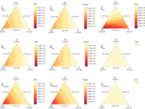
Varying combinations of relative pairs:Finally, we studied the effect of relative pair combinations in a sample, using allele frequencies at the ATCT003, DXS1068, and GATA48H04 loci. Only the results for the highest heterozygosity locus, ATCT003, are shown; as was true in the previous section, each locus yielded similar results. For each locus, we examined each of the 231 possible divisions of exactly 20 full-sib pairs into male– male (t1), male–female (u2), and female–female (v2)

pairs. Figure 4 displays the MSE, variance, and bias squared of the three estimators, calculated analytically using the variance approximation (Equation 18), for var-ious combinations oft1,u2, andv2pairs for the ATCT003

locus. Variance was highest forHˆreduced, because it had

the smallest sample of alleles. For all estimators, var-iance was highest where the configuration of full-sibs had mostly male–male pairs, again due to the smaller sample of alleles.H˜fullandHˆreducedwere unbiased across

the space of possible combinations.Hˆfullshowed a trend

in bias squared in which configurations with a greater proportion of males had higher bias squared, as is predicted analytically from the smaller sample size

Figure3.—Mean squared error as a function of sample size (number of pairs¼number of individuals/2), calculated

analyt-ically using the variance approximation (Equation 18 inserted into Equations 15 and 16), on the basis of allele frequencies at the DXS1068 locus (H¼0.7344) for male–female relative pairs in which the females were removed to evaluateHˆreduced. The range of

(Equation 14). For all configurations, the bias squared ofHˆfull was greater than that for the other estimators.

Among the three estimators, MSE was highest for ˆ

Hreduced. Similarly to the observation for variance, MSE

was greatest for configurations with a high proportion of male–male pairs. Although H˜full performed slightly

worse in having a greater variance compared toHˆfull, it

had a slightly lower MSE due to its lower bias. More generally, althoughH˜fullperformed better in the setting

of Figure 4, the exact formula can be used to determine which estimator has lowest MSE for a given scenario.

Application to data: We next investigated the behav-ior of our estimator using X-chromosomal SNP data sets of 485 individuals and 446 unrelated individuals (see Data). Table 4 displays the relative pairs in the sample of 485 individuals. Because we analyzed the estimators separately by population, the subscripts of 485 and 446

refer to whether or not relatives were included in a calculation, not to the actual numbers of individuals in that calculation. In the same manner as in DeGiorgio

and Rosenberg(2009), we tookHˆ₄₄₆ for each

popula-tion to be a proxy for true heterozygosity, because this quantity provided an unbiased estimate when no rela-tives were included in the sample. Note that removed individuals belonged only to pairs related through the X chromosome; individuals related only autosomally (such as male–male parent–offspring pairs) were in-cluded in the reduced sample. In our analysis, we compared the means of H˜485 and Hˆ485 across the

13,052 loci to the corresponding mean ofHˆ446.

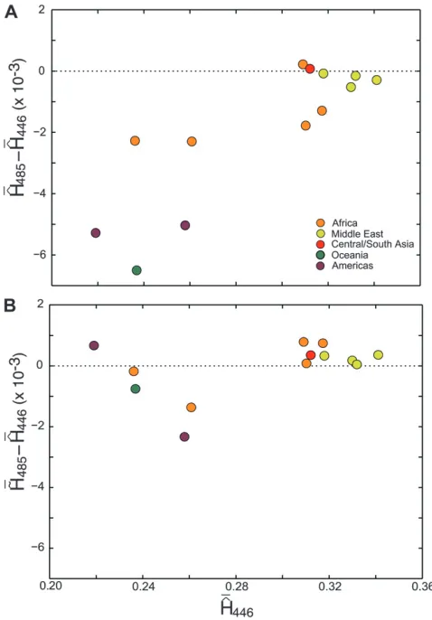
Figure 5 compares the difference between the mean ofHˆ485across loci (Hˆ485) and the mean ofHˆ446(Hˆ446)

with the difference between the mean of H˜485 (H˜485)

and the mean ofHˆ446(Hˆ446). As Figure 5A shows,Hˆ485

Figure_{4.—Mean squared error (MSE), variance, and bias squared ofH}ˆ

full,H˜full, andHˆreduced, calculated analytically using the

variance approximation (Equation 18 inserted into Equations 15 and 16), as functions of the configuration oft1male–male

(F¼1

2),u1male–female (F¼12), andy2female–female (F¼38) pairs in 20 total relative pairs, on the basis of allele frequencies

at the ATCT003 locus (H¼ 0.7794). Each row displays a different estimator and each column displays a different statistic. The three vertices of each triangle represent 20 male–male, 20 male–female, and 20 female–female full-sib pairs. The numbers on the scale indicate the cutoff values for colors. Note that unlike for the other two estimators, the scale for bias squared ofHˆfull

includes nonzero values. The black dot on each graph (except the bias squared graphs forH˜fullandHˆreduced) represents the largest

generally yields a lower heterozygosity estimate than ˆ

H446 due to the downward bias caused by related

individuals. Applying H˜485 reduces the magnitude of

the difference between the estimate of heterozygosity in sets with and without relatives (Figure 5B), andH˜485

yields values that are not consistently lower than those of ˆ

H446. It is important to note that because 15 of 45 of the

relative pairs in the data have an uncertain second-degree relationship (t3, u5, or v5), H˜485 might have

overcorrected bias in cases in which the individuals were not related via the X chromosome and undercorrected bias in cases in which the individuals actually were related on the X chromosome.

A Wilcoxon signed-rank test was used to evaluate the differences between Hˆ485 and Hˆ446 applied to the 13

populations that contained relatives (see Table 4). This test yielded aP-value of 0.0024, indicating that the inclusion of relatives had a significant impact on the estimation of heterozygosity usingH. In contrast, the Wilcoxon signed-ˆ rank comparison ofH˜485 and Hˆ446 yielded a P-value of

0.6355, indicating that the inclusion of relatives did not significantly alter the estimation of heterozygosity whenH˜ was used. The mean difference_H˜_485Hˆ_446(8.04933 105_{) and the mean absolute difference jH}˜

485Hˆ446j

(6.31593 104_{) were smaller across the 13 populations}

than the mean difference (1.93933103_{) and the mean}

absolute difference (1.9849 3 103_{), H}ˆ

446Hˆ485 and

j_Hˆ_446Hˆ_{485j, respectively.}

We also investigated the behavior of H˜ and Hˆ with regard to variance for the 13 populations that contained relatives. We compared Hˆ485Hˆ446 and H˜485Hˆ446,

which we used as proxies for bias, following the methods of DeGiorgioand Rosenberg(2009), and the standard

deviations of the two estimators applied with relatives included. From Figure 6, we observe that while there was a sizeable difference in the bias proxy betweenHˆ485

and H˜485, there was only a small difference in

stan-dard deviation. This result is compatible with the res-ults from our analytical computations, which suggest that H˜ corrects bias without substantially increasing variance.

DISCUSSION

Our estimator,H, is an effective tool for assessing the˜ gene diversity of a sample of arbitrary ploidy containing related or inbred individuals. It can be used to provide unbiased estimates of expected heterozygosity when the inbreeding and kinship coefficients of sampled

individ-Figure 5.—Comparison of the difference between the

mean of_Hˆ₄₈₅across loci and the mean of_Hˆ₄₄₆with the differ-ence between the mean of_H˜₄₈₅and the mean of_Hˆ₄₄₆. (A) The difference between the mean ofHˆ485and the mean ofHˆ446for

each of the 13 populations containing relatives (Table 4). (B) The difference between the mean ofH˜485and the mean ofHˆ446

for each of the 13 populations. The estimators were applied to a data set of 13,052 SNP loci with 485 individuals belonging to 29 populations, and the results for the 13 populations with rel-atives are shown. Included in the set of 485 individuals was a subset of 446 individuals that contained no relatives. The sub-scripts of 485 and 446 refer to whether or not relatives were in-cluded, not to the actual number of individuals in the calculation. Each data point represents one population, with color indicating the geographic region of that population. The dotted line indicates a difference of zero.

TABLE 4

Types of relative pairs in populations from the data set of 485 individuals reported by JAKOBSSONet al.(2008)

t1 t2 t3 u1 u2 u3 u4 u5 v1 v2 v3 v4 v5

Bantu (Kenya) 1

Bedouin 1 1

Biaka Pygmy 1 2 1 2

Druze 2 1 2

Kalash 1

Mandenka 1 1

Maya 1 1 2

Mbuti Pygmy 1 1

Melanesian 1 3 2 2 1

Mozabite 1

Palestinian 1 1

Pima 1 1 1 1 1 1

Yoruba 1 1 1 1

Total 4 1 5 7 6 1 0 3 5 5 0 1 7

uals are known. We found that the unbiasedness of the diploid estimator of DeGiorgio and Rosenberg

(2009) extends to a much more general set of scenarios, provided that kinship coefficients are appropriately weighted by ploidy in the computation.

Here, we evaluated the properties of H˜ in the spe-cific case of the human X chromosome. Through our analytical calculations, we have shown that, similarly to the DeGiorgioand Rosenberg(2009) estimator in the

diploid case, the performance ofH˜ is generally supe-rior to that of Hˆ when the sample to which the esti-mators are applied contains relatives.H˜accounts for the bias introduced by relatedness while simultaneously maintaining comparable MSE and variance toH. Ourˆ estimator also performs well compared toHˆ when ap-plied to data from human populations. While the true heterozygosity of each population is not known, when we compared H˜ and Hˆ to an approximation of true heterozygosity, with Hˆ applied to the data set with no related individuals, we found that the difference be-tween the estimate when relatives were included and when relatives were not included was significantly smaller forH. Because the reduction in this proxy for˜ bias is accompanied by only a small increase in standard deviation, we argue that H˜ should often be preferred overHˆ in the estimation of gene diversity in a sample containing relatives.

In addition to developing theH˜ estimator for gene diversity, we also determined the analytical variance of

our estimator, allowing us to theoretically evaluate the properties of H. We also developed an approximation˜ for variance (Equation 18) that is simpler to compute and that is applicable when each individual has at most one relative in the sample. Knowledge of the theoretical variance can further allow investigators to evaluate the circumstances under whichH˜ applied to a full sample, including relatives, is superior to usingHˆwith a reduced sample in which members of relative pairs have been removed. For example, Figure 2 indicates that removing relatives will provide a lower MSE of the heterozygosity estimate in some cases. However, Figure 4 suggests that

˜

Hfullyields a lower MSE thanHˆreducedexcept in the small

fraction of relative–pair combinations that contain large numbers ofu1pairs. Thus, we propose that in most cases

the use of H˜ on a sample set that includes related individuals affords a better estimate of gene diversity than applyingHˆ on a sample that contains no relatives and that investigators can use the theoretical variance of

˜

Hto determine whether a given situation is likely to be among the exceptions.

We thank Laurent Excoffier and three anonymous reviewers for their valuable comments. This work was supported by National Institutes of Health (NIH) grant R01 GM081441, NIH training grant T32 GM070449, a University of Michigan Rackham Merit Fellowship, and grants from the Burroughs Wellcome Fund and the Alfred P. Sloan Foundation.

LITERATURE CITED

Buteler_{, M. I., R. L. J}arret_{and D. R. L}a_Bonte_{, 1999 Sequence}

characterization of microsatellites in diploid and polyploid Ipo-moea.Theor. Appl. Genet.99:123–132.

Cockerham, C. C., 1971 Higher order probability functions of

iden-tity of alleles by descent. Genetics69:235–246.

Cotterman, C., 1940 A calculus for statistico-genetics. Ph.D. Thesis,

Ohio State University, Columbus, OH. Reprinted inGenetics and Social Structure, pp. 157–272, edited by P. Ballonoff. Dowden,

Hutchinson & Ross, Stroudsburg, PA, 1974.

De_Giorgio_{, M., and N. A. R}osenberg_{, 2009 An unbiased estimator}

of gene diversity in samples containing related individuals. Mol. Biol. Evol.26:501–512.

Gillois, M., 1965 Relation d’identite´ en ge´ne´tique. Ann. Inst. H.

Poincare´ Sect. B2:1–94 (in French).

Harris, D. L., 1964 Genotypic covariances between inbred relatives.

Genetics50:1319–1348.

Jacquard, A., 1974 The Genetic Structure of Populations.Springer, New

York.

Jakobsson, M., S. W. Scholz, P. Scheet, J. R. Gibbs, J. M. VanLiere

et al., 2008 Genotype, haplotype and copy-number variation in worldwide human populations. Nature451:998–1003.

Lange, K., 2002 _{Mathematical and Statistical Methods for Genetic}

Anal-ysis, Ed. 2. Springer, New York.

Nei, M., 1973 Analysis of gene diversity in subdivided populations.

Proc. Natl. Acad. Sci. USA70:3321–3323.

Nei, M., and A. K. Roychoudhury, 1974 Sampling variances of

het-erozygosity and genetic distance. Genetics76:379–390. Ramachandran, S., N. A. Rosenberg, M. W. Feldmanand J. Wakeley,

2008 Population differentiation and migration: coalescence times in a two-sex island model for autosomal and X-linked loci. Theor. Popul. Biol.74:291–301.

Reiland_{, J., S. H}odge_{and M. A. F. N}oor_{, 2002 Strong founder}

effect inDrosophila pseudoobscura colonizing New Zealand from North America. J. Hered.93:415–420.

Ritland, K., 1996 Estimators for pairwise relatedness and

individ-ual inbreeding coefficients. Genet. Res. Camb.67:175–185.

Figure 6.—Comparison of the difference between the

mean of the estimator and the mean ofHˆ446and standard

de-viation of the estimator, for the estimators H˜485 and Hˆ485.

These estimators were applied to a full data set of 13,052 X chromosome SNP loci with 485 individuals belonging to 29 populations, whereas 446 individuals were included in the re-duced data set that contained no relatives. Only the 13 pop-ulations containing relatives are shown. The subscripts 485 and 446 refer to whether or not relatives were included, not to the actual number of individuals in the calculation. Open and solid points represent the estimates forHˆ485and

˜

H485, respectively. The dotted line indicates a difference of

Rosenberg, N. A., 2006 Standardized subsets of the HGDP-CEPH

Human Genome Diversity Panel, accounting for atypical and duplicated samples and pairs of close relatives. Ann. Hum. Genet.70:841–847.

Rousset, F., 2002 Inbreeding and relatedness coefficients: What do

they measure? Heredity88:371–380.

Thompson, E. A., 1974 Gene identities and multiple relationships.

Biometrics30:667–680.

Weir_{, B. S., 1989 Sampling properties of gene diversity, pp. 23–42 in}

Plant Population Genetics, Breeding and Genetic Resources, edited by

A. H. D. Brown, M. T. Clegg, A. L. Kahlerand B. S. Weir

Sinauer Associates, Sunderland, MA.

Weir, B. S., 1996 Genetic Data Analysis II.Sinauer Associates,

Sunder-land, MA.

Communicating editor: L. Excoffier

APPENDIX A

In this section, we present proofs for Equations 9, 11, 12, and 13.

Proof of Equation9. Applying the definition ofˆpiand using Equation 8, we have

E _ˆp2

i ¼

1

ðPgb¼1nbmbÞ2

Xg

a¼1

Xg

b¼1

Xna

j¼1

Xnb

k¼1

E _XðiÞ ða;jÞX

ðiÞ ðb;kÞ

h i

¼ 1

ðPg_b¼1nbmbÞ2

Xg

a¼1

Xg

b¼1

Xna

j¼1

Xnb

k¼1

Xma

‘¼1

Xmb

t¼1

E _AðiÞ ða;jÞ;‘A

ðiÞ ðb;kÞ;t

h i

¼ 1

ðPg_b¼1nbmbÞ2

Xg

a¼1

Xg

b¼1

Xna

j¼1

Xnb

k¼1

Xma

‘¼1

Xmb

t¼1

ðF_ða;jÞðb;kÞpið1piÞ1p2iÞ

¼ 1

ðPg_b¼1nbmbÞ2

Xg

a¼1

Xg

b¼1

Xna

j¼1

Xnb

k¼1

mambðFða;jÞðb;kÞpið1piÞ1p2iÞ

¼ð

Pg

b¼1nbmbÞ2 ðPg_b¼1nbmbÞ2

F2pið1piÞ1ð

Pg

b¼1nbmbÞ2 ðPg_b¼1nbmbÞ2

p2_i

¼F2pið1piÞ1p2i: n

Proof of Equation11.ˆP½IBS ¼PI

i¼1ˆp2i. We only need to show thatP½IBD ¼F2. Note that while we writeˆP½IBSas an

estimate,P[IBD] depends only on quantities that are treated as known with certainty and we write it as a known quantity itself. Consider two alleles from the sample (that are not necessarily distinct). LetC(a,j)(b,k)denote the event that the

first of the two alleles is from individual (a,j) and the second is from individual (b,k), where (a,j) and (b,k) are not necessarily distinct. Supposing that the two alleles are drawn uniformly at random from the sample, with replacement, letPC(a,j)(b,k)

denote the probability of eventC(a,j)(b,k). LetP

IBDjC(a,j)(b,k)

be the probability that two alleles are IBD given that the first allele is chosen from individual (a,j) and the second is chosen from individual (b,k). Then

P_{½IBD ¼}X

g

b¼1

Xnb

k¼1

P_{IBDjCðb;kÞðb;kÞ}P_{Cðb;kÞðb;kÞ}1X

nb

j¼1

Xnb

k¼1

k6¼j

P_{IBDjCðb;jÞðb;kÞ}P_{Cðb;jÞðb;kÞ}

8 > > < > > :

9 > > = > > ;

1 X

g

a¼1

Xg

b¼1

b6¼a

Xna

j¼1

Xnb

k¼1

P_{IBDjCða;jÞðb;kÞ}P_{Cða;jÞðb;kÞ}:

P_{Cða;jÞðb;kÞ ¼} ma

Pg c¼1ncmc

mb

Pg c¼1ncmc

¼ mamb

ðPg_c¼1ncmcÞ2

P_{IBDjCða;jÞ ðb;kÞ¼}Fða;jÞ ðb;kÞ:

It follows that

P_{½IBD ¼}X

g

b¼1

Xnb

k¼1

Fðb;kÞðb;kÞ

m2_b

ðPg_c¼1ncmcÞ2

1X

nb

j¼1

Xnb

k¼1

k6¼j

Fðb;jÞðb;kÞ

m2_b

ðPg_c¼1ncmcÞ2

8 > > > > > < > > > > > : 9 > > > > > = > > > > > ; 1 X g

a¼1

Xg

b¼1

b6¼a

Xna

j¼1

Xnb

k¼1

Fða;jÞðb;kÞ

mamb ðPg_c¼1ncmcÞ2

¼ 1

ðPg_b¼1nbmbÞ2

Xg

a¼1

Xg

b¼1

Xna

j¼1

Xnb

k¼1

mambFða;jÞ ðb;kÞ

¼F2: n

Proof of Equation12. For anmb-ploid individualk,F(b,k)(b,k)¼1/mb1(11/mb)f(b,k)¼(1/mb)[11(mb1)f(b,k)]. Note

that F_(a,j)(b,k) ¼0 if individuals (a, j) and (b, k) are unrelated. We can then break F₂ into three components, considering three different types of pairs of individuals: same group–same individual, same group–different individual, and different group. Therefore

F2¼ 1

ðPg_b¼1nbmbÞ2

Xg

a¼1

Xg

b¼1

Xna

j¼1

Xnb

k¼1

mambFða;jÞðb;kÞ

¼ 1

ðPg_b¼1nbmbÞ2

Xg

b¼1

Xnb

k¼1

m2_bFðb;kÞðb;kÞ12

Xg

b¼1

X

nb1

j¼1

Xnb

k¼j11

m2_bFðb;jÞðb;kÞ

"

1 2X

g1

a¼1

Xg

b¼a11

Xna

j¼1

Xnb

k¼1

mambFða;jÞðb;kÞ

#

¼ 1

ðPg_b¼1nbmbÞ2

Xg

b¼1

Xnb

k¼1 m2_b 1

mb

11ðmb1Þfðb;kÞ

12X

g

b¼1

X

R2Gb;b

m2_bh_RF_R

2 4

1 2X

g1

a¼1

Xg

b¼a11

X

R2Ga;b

mambhRFR

3 5

¼ 1

ðPg_b¼1nbmbÞ2

Xg

b¼1 nbmb1

Xg

b¼1

nbmbðmb1Þfb12

Xg

b¼1

X

R2Gb;b

m2_bh_RF_R

2 4

1 2X

g1

a¼1

Xg

b¼a11

X

R2Ga;b

mambhRFR

3

5: n

Proof of Equation13. First we note that

1F2¼

D

ðPg_b¼1nbmbÞ2 :

˜ H¼ð

Pg

b¼1nbmbÞ2

D 1

XI

i¼1 ˆp2

i

!

:

Rearranging Equation 3 we get

1X I

i¼1 ˆp2

i ¼

Pg

b¼1nbmb1

Pg b¼1nbmb

ˆ H; from which

˜ H¼ð

Pg

b¼1nbmbÞ2

D

Pg

b¼1nbmb1

Pg b¼1nbmb

ˆ H

¼ð

Pg

b¼1nbmbÞðPbg¼1nbmb1Þ

D Hˆ: n

APPENDIX B

In this section, we present results that aid in the derivation of the variance of our gene diversity estimator. Lemma 3 derives certain expectations involving four alleles. These expectations are used to calculate the variance and covariance of squared allele frequency estimates in Lemma 4. Lemma 4 is then used to prove the variance formula in Theorem 2 when related and inbred individuals are included in a sample.

Lemma 3.Consider a locus with I distinct alleles,allele frequencies p_i2 [0, 1],and PI

i¼1pi¼1.Suppose a sample from a population has g groups,each with different ploidy,and nbmb-ploid individuals in group b,b¼1, 2,. . .,g,each of whom is possibly inbred and related to other individuals in the sample. Consider the‘th allele of individual(a,j),the tth allele of individual (b,k),the‘9th allele of individual(a9,j9),and the t9th allele of individual(b9,k9).For clarity,let w¼(a,j),x¼(b,k),y¼

(a9,j9),and z¼(b9,k9).Then for allelic types i and i96¼i,

E _AðiÞ w;‘A

ðiÞ x;tA

ðiÞ y;‘9A

ðiÞ z;t9

h i

¼F_wxyzpi

1 F_wxy1F_wxz1F_wyz1F_xyz1F_wx;yz1Fwy;xz1Fwz;xy7Fwxyz

p2_i 1½12Fwxyz1ðFwx1Fwy1Fwz1Fxy1Fxz1FyzÞ

3ðF_wxy1F_wxz1F_wyz1F_xyzÞ 2ðF_wx;yz1Fwy;xz1Fwz;xyÞp3_i

1½11ðFwx;yz1Fwy;xz1Fwz;xyÞ12ðFwxy1Fwxz1Fwyz1FxyzÞ

6F_wxyz ðF_wx1F_wy1F_wz1F_xy1F_xz1F_yzÞp4_i ðB1Þ

E _AðiÞ w;‘A

ðiÞ x;tA

ði9Þ y;‘9A

ði9Þ z;t9

h i

¼ Fwx;yzFwxyz

pipi91 2Fwxyz1Fwx ðFwxy1FwxzÞ Fwx;yz

pip2i9

1 2F_wxyz1F_yz ðF_wyz1F_xyzÞ F_wx;yz

p2_ipi9

1½11F_wx;yz1Fwy;xz1Fwz;xy12ðFwxy1Fwxz1Fwyz1FxyzÞ

6Fwxyz ðFwx1Fwy1Fwz1Fxy1Fxz1FyzÞp2ip2i9: ðB2Þ

Proof.We need to evaluate

E _AðiÞ w;‘A

ðiÞ x;tA

ði9Þ y;‘9A

ði9Þ z;t9

h i

¼X

15

s¼1

DsP AðwiÞ;‘¼1;A

ðiÞ x;t ¼1;A

ði9Þ y;‘9 ¼1;A

ði9Þ

z;t9 ¼1jS¼s

h i

;

X15

s¼1 D_s¼1

Fwxyz¼D1 F_wxy¼D11D2 F_wxz¼D₁1D₃ Fwyz¼D11D4 F_xyz¼D₁1D₅ Fwx;yz¼D11D6 F_wy;xz¼D11D9 F_wz;xy¼D11D12

F_wx ¼D11D21D31D61D7 F_wy¼D₁1D₂1D₄1D₉1D₁₀ Fwz¼D11D31D41D121D13

F_xy¼D₁1D₂1D₅1D₁₂1D₁₄ F_xz¼D₁1D₃1D₅1D₉1D₁₁

F_yz¼D11D41D51D61D8: ðB3Þ Note that theD-coefficients above are identical to thed-coefficients in Cockerham(1971). Also, theF-coefficients

involving two individuals, three individuals, and pairs of pairs of individuals are identical to Cockerham’su-,g-, and D-coefficients, respectively (Cockerham1971). Ifi9¼i, we get

E _AðiÞ w;‘A

ðiÞ x;tA

ðiÞ y;‘9A

ðiÞ z;t9

h i

¼D1pi1ðD21D31D41D51D61D91D12Þp2i: ðB4Þ

Ifi6¼i9, we get

E _AðiÞ w;‘A

ðiÞ x;tA

ði9Þ y;‘9A

ði9Þ z;t9

h i

¼D6pipi91D7pip2i91D8p2ipi91D15p2ip2i9: ðB5Þ

The desired result follows by substituting Equation B3 into Equations B4 and B5. n

Note that expressions mathematically identical to Equations B1 and B2 except with different notation appear in Table 1 of Cockerham(1971). However, a slight conceptual difference is that our formulas involve an expectation of

a product among four arbitrary alleles, not necessarily four alleles in two pairs of diploid genotypes. We now use Lemma 3 to derive Var ˆp2

i and Cov ˆp

2

i; ˆp

2

i9

.

Lemma4.Consider a locus with I distinct alleles,allele frequencies p_i2[0, 1],andPI

i¼1pi¼1.Suppose a sample from a population has g groups,each with different ploidy,and nbmb-ploid individuals in group b,b¼1, 2,. . .,g,each of whom is possibly inbred and related to other individuals in the sample. Then for allelic types i and i96¼i,

E _ˆp4

i ¼F4pi1 4F313F2;27F4

p2_i 1 12F416F212F36F2;2

p3_i

1113F2;218F36F46F2p4_i ðB6Þ

E _ˆp2

iˆp2i9

¼F_2;2F₄pipi91 2F41F22F3F2;2

pip2i91 2F41F22F3F2;2

p2_ipi9

1 113F2;218F36F46F2

p2_ip2_i9 ðB7Þ

and therefore

Var ˆp2

i ¼F4pi1 4F313F2;27F4F22

p_i2112F414F212F2212F36F2;2p3_i 1 3F₂;218F36F44F2F22

p4_i ðB8Þ

Covðˆp2

i; ˆp2i9Þ ¼ F2;2F4F22

pipi91 2F41F222F3F2;2

pip2i9

1 2F41F222F3F2;2

p2_ipi91 3F2;218F36F44F2F22

p2_ip2_i9: ðB9Þ

E _ˆp4

i ¼

1

ðPg_b¼1nbmbÞ4

Xg

a¼1

Xg

b¼1

Xg

a9¼1

Xg

b9_¼1

Xna

j¼1

Xnb

k¼1

Xna9

j9_¼1

Xnb9

k9_¼1

Xma

l¼1

Xmb

t¼1

Xma9

l9¼1

Xmb9

t9¼1 3E AððiaÞ;jÞ;‘A

ðiÞ ðb;kÞ;tA

ðiÞ ða9;j9Þ;‘9A

ðiÞ ðb9;k9Þ;t9

h i

¼ 1

ðPg_b¼1nbmbÞ4

Xg

a¼1

Xg

b¼1

Xg

a9¼1

Xg

b9_¼1

Xna

j¼1

Xnb

k¼1

Xna9

j9¼1

Xnb9

k9¼1

mambma9mb9

3fF_ða;jÞðb;kÞða9;j9Þðb9;k9Þpi

1 F_ða;jÞðb;kÞða9;j9Þ1Fða;jÞðb;kÞðb9;k9Þ1Fða;jÞða9;j9Þðb9;k9Þ1Fðb;kÞða9;j9Þðb9;k9Þ

1Fða;jÞðb;kÞ;ða9;j9Þðb9;k9Þ1Fða;jÞða9;j9Þ;ðb;kÞðb9;k9Þ1Fða;jÞðb9;k9Þ;ðb;kÞða9;j9Þ

7Fða;jÞðb;kÞða9;j9Þðb9;k9Þ

p2_i 112Fða;jÞðb;kÞða9;j9Þðb9;k9Þ

1Fða;jÞðb;kÞ1Fða;jÞða9;j9Þ1Fða;jÞðb9;k9Þ1Fðb;kÞða9;j9Þ1Fðb;kÞðb9;k9Þ1Fða9;j9Þðb9;k9Þ

3ðFða;jÞðb;kÞða9;j9Þ1Fða;jÞðb;kÞðb9;k9Þ1Fða;jÞða9;j9Þðb9;k9Þ1Fðb;kÞða9;j9Þðb9;k9ÞÞ 2ðFða;jÞðb;kÞ;ða9;j9Þðb9;k9Þ1Fða;jÞða9;j9Þ;ðb;kÞðb9;k9Þ1Fða;jÞðb9k9Þ;ðb;kÞða9;j9ÞÞ

p3_i 1½11Fða;jÞðb;kÞ;ða9;j9Þðb9;k9Þ1Fða;jÞða9;j9Þ;ðb;kÞðb9;k9Þ1Fða;jÞðb9;k9Þ;ðb;kÞða9;j9Þ

12ðFða;jÞðb;kÞða9;j9Þ1Fða;jÞðb;kÞðb9;k9Þ1Fða;jÞða9;j9Þðb9;k9Þ1Fðb;kÞða9;j9Þðb9;k9ÞÞ 6Fða;jÞðb;kÞða9;j9Þðb9;k9Þ

ðFða;jÞðb;kÞ1Fða;jÞða9;j9Þ1Fða;jÞðb9;k9Þ1Fðb;kÞða9;j9Þ1Fðb;kÞðb9;k9Þ

1F_ða9;j9Þðb9;k9ÞÞp4ig ¼ F4pi1 4F313F2;27F4

p2_i 1 12F416F212F36F2;2

p3_i 1 113F2;218F36F46F2

p4_i: For the case with allelesiandi96¼i, we have

E _ˆp2

iˆp2i9

¼ 1

ðPg_b¼1nbmbÞ4

Xg

a¼1

Xg

b¼1

Xg

a9¼1

Xg

b9_¼1

Xna

j¼1

Xnb

k¼1

Xna9

j9¼1

Xnb9

k9¼1

Xma

‘¼1

Xmb

t¼1

Xma9

‘9¼1

Xmb9

t9¼1 3E AððiaÞ;jÞ;‘A

ðiÞ ðb;kÞ;tA

ði9Þ ða9;j9Þ;‘9A

ði9Þ ðb9;k9Þ;t9

h i

¼ 1

ðPg_b¼1nbmbÞ4

Xg

a¼1

Xg

b¼1

Xg

a9¼1

Xg

b9_¼1

Xna

j¼1

Xnb

k¼1

Xna9

j9¼1

Xnb9

k9¼1

mambma9mb9

3 Fða;jÞðb;kÞ;ða9;j9Þðb9;k9ÞFða;jÞðb;kÞða9;j9Þðb9;k9Þ

pipi9

1 2Fða;jÞðb;kÞða9;j9Þðb9;k9Þ1Fða;jÞðb;kÞ

Fða;jÞðb;kÞða9;j9Þ1Fða;jÞðb;kÞðb9;k9ÞFða;jÞðb;kÞ;ða9;j9Þðb9;k9Þpip2i9

1 2F_ða;jÞðb;kÞða9;j9Þðb9;k9Þ1Fða9;j9Þðb9;k9Þ

Fða;jÞða9;j9Þðb9;k9Þ1Fðb;kÞða9;j9Þðb9;k9Þ

Fða;jÞðb;kÞ;ða9;j9Þðb9;k9Þ

p2_ipi9

1 11Fða;jÞðb;kÞ;ða9;j9Þðb9;k9Þ1Fða;jÞða9;j9Þ;ðb;kÞðb9;k9Þ1Fða;jÞðb9;k9Þ;ðb;kÞða9;j9Þ

1 2Fða;jÞðb;kÞða9;j9Þ1Fða;jÞðb;kÞðb9;k9Þ1Fða;jÞða9;j9Þðb9;k9Þ1Fðb;kÞða9;j9Þðb9;k9Þ 6Fða;jÞðb;kÞða9;j9Þðb9;k9Þ

Fða;jÞðb;kÞ1Fða;jÞða9;j9Þ1Fða;jÞðb9;k9Þ1Fðb;kÞða9;j9Þ1Fðb;kÞðb9;k9Þ

1Fða9;j9Þðb9;k9Þ

p2_ip2_i9g ¼ F2;2F4

pipi91 2F41F22F3F2;2

pip2i91 2F41F22F3F2;2

p2_ipi9

1 113F₂;218F36F46F2

p2_ip2_i9: