ABSTRACT
HO, YANG. Graph Characteristics and Branch-and-Reduce Algorithms for Minimum Vertex Cover. (Under the direction of Dr. Matthias Stallmann).
The Minimum Vertex Cover problem is a well known NP-Completeproblem. Branching al-gorithms are commonly used to solve Minimum Vertex Cover and related problems. Many reduction rules have been developed to help reduce the problem instance and improve the
perfor-mance of branching algorithms. Over the years, the reduction rules have become more sophisticated and complex. Although many of these reductions have been shown to be effective in theory and in
practice, there are circumstances where the overhead of applying these reductions is greater than
the extent they reduce the problem instance.
In this thesis, we look to determine graph characteristics that can be used to predict the
effective-ness of certain reductions. We focus on how the number of odd cycles in a graph relates to the
effectiveness of theLPreduction. We also focus on how the degree variance and density affects the degree-one and dominance reductions. For our experiments we use a variety of generated instances
and benchmarks. Our results show that theLPreduction is most effective when the number of odd cycles is low; in addition, the degree-one and dominance reduction combination is most effective when the degree variance is high or when the density is very low. Ultimately, we hope to use our
results to engineer a better solver for Minimum Vertex Cover; ideally, the solver will automat-ically analyze the graph and makes decisions about which reduction to apply based on the degree
Graph Characteristics and Branch-and-Reduce Algorithms for Minimum Vertex Cover
by Yang Ho
A thesis submitted to the Graduate Faculty of North Carolina State University
in partial fulfillment of the requirements for the Degree of
Master of Science
Computer Science
Raleigh, North Carolina
2018
APPROVED BY:
Dr. Blair Sullivan Dr. Steffen Heber
BIOGRAPHY
Yang Ho was born in Lyndhurst, New Jersey. His family moved down to Cary, North Carolina when
he was 4 years old and have lived there ever since. He completed his undergraduate education at
ACKNOWLEDGEMENTS
I would like to thank my advisor, Dr. Matthias Stallmann, for his help and guidance. I am also
thankful for my other committee members: Dr. Sullivan, and Dr. Heber. Lastly, I am grateful for
TABLE OF CONTENTS
List of Tables . . . vi
List of Figures . . . vii
Chapter 1 Introduction . . . 1
1.1 Terminology . . . 1
1.2 Minimum Vertex Cover and Related Problems . . . 2
1.3 Branching Algorithms . . . 2
1.3.1 Generic Branching Algorithms forMinimum Vertex Cover . . . 2
1.3.2 Measure and Conquer Analysis . . . 3
1.3.3 Bottom-Up . . . 4
1.4 Summary and Outline . . . 4
Chapter 2 Reduction Rules. . . 6
2.1 Definitions and Terminology . . . 6
2.2 Unconfined vertices . . . 6
2.3 Folding . . . 8
2.3.1 Completek-Independent Sets . . . 8
2.3.2 Fomin Folding . . . 9
2.4 Alternative Structures . . . 10
2.5 LP Reduction . . . 12
2.5.1 LPRelaxation . . . 12
2.5.2 Extreme optimal solutions . . . 13
2.5.3 Lower bounds . . . 14
2.6 Concluding Remarks . . . 14
Chapter 3 Implementation Details . . . 15
3.1 Implementation Overview . . . 15
3.1.1 Reductions . . . 17
3.1.2 Lower Bounds . . . 19
3.1.3 Branching . . . 20
3.2 Tracing and Instrumentation . . . 21
3.3 Concluding Remarks . . . 26
Chapter 4 Graph Characteristics . . . 27
4.1 Measures and Characteristics . . . 27
4.1.1 Odd Cycles . . . 28
4.1.2 Degree Distribution . . . 33
4.1.3 Edge Density . . . 35
4.2 Graph Classes . . . 36
4.2.1 Augmented Odd Cycle Graphs . . . 36
4.2.2 Other Generated Graphs . . . 39
4.2.3 Benchmarks . . . 43
4.3 Experimental Results . . . 53
4.3.1 Experimental Setup . . . 53
4.3.3 Degree Distribution and Degree-One/Dominance Reductions . . . 61
4.3.4 Edge Density and Degree-One/Dominance Reductions . . . 65
4.4 Concluding Remarks . . . 69
Chapter 5 Conclusions and Future Work . . . 70
5.1 Validation of Hypotheses . . . 70
5.2 Future Work . . . 71
BIBLIOGRAPHY . . . 73
APPENDIX . . . 75
Appendix A DIMACS Instances . . . 76
A.1 Random . . . 76
A.2 Embedded Clique . . . 77
A.3 Other . . . 77
LIST OF TABLES
Table 1.1 Some results and key papers . . . 4
Table 3.1 Time complexity for the reductions presented. . . 18
Table 3.2 Summary of runtime options available in our enhanced vcsolver. . . 22
Table 4.1 Random graphs: Measure values. . . 40
Table 4.2 Geometric and Geo-wrap graphs: Measure values. . . 41
Table 4.3 Random DIMACS: Measure values for benchmarks taken from various random graph generators. . . 43
Table 4.4 Clique DIMACS: Measure values for benchmarks with a clique embedded into the graph. . . 44
Table 4.5 Other DIMACS: Measure values for benchmarks based on other problems or ap-plications. . . 44
Table 4.6 Hamming graphs: Measure values. . . 48
Table 4.7 Coding-error graphs: Measure values. . . 48
Table 4.8 Coding-error graphs: Measure value averages and standard deviations. . . 49
Table 4.9 Real-world sparse networks: Measure values sorted by edge density (ED). . . 51
Table 4.10 Hamming graphs: Measure values and runtimes. . . 58
Table 4.11 Coding-error graphs: Measure values and runtimes. . . 58
Table 4.12 Selection of DIMACS instances: Measure values and runtimes. . . 59
Table 4.13 Real-world sparse networks: Measure values and runtimes. . . 62
Table 4.14 Random graphs: Measure values and runtimes. . . 66
Table 4.15 Delaunay triangulation graphs: Measure values and runtimes. . . 68
Table A.1 Parameter values for p hatV-X instances . . . 76
LIST OF FIGURES
Figure 2.1 Vertexc is confined bySc={c, g, i} . . . 8
Figure 2.2 Example of a twin (note that no vertex is unconfined). . . 9
Figure 2.3 Example of folding a vertex v . . . 10
Figure 2.4 ais a funnel in both examples . . . 11
Figure 2.5 A desk . . . 11
Figure 3.1 Example of how to split a cycle: 1,2,3,4,5,6 is a part of a cycle cover. After splitting, the cycle cover now includes 1,5,6 and 2,3,4. . . 20
Figure 3.2 Example of a mirror and mirror branching. . . 21
Figure 3.3 Example output of vcsolver. . . 21
Figure 3.4 Example of the basic statistics our modified version reports. . . 23
Figure 3.5 Example of the some of the additional statistics our modified version reports. . . 23
Figure 3.6 Example trace output. . . 24
Figure 3.7 Example of a status vector. . . 24
Figure 3.8 Example of branching and the resulting trace outputs. In this example, only the degree-one reduction is used. . . 25
Figure 4.1 phat-1 series: Runtime as a function of the number of vertices. The reductions presented are: the degree-one+dominance reductions (DD), the LP reduction (LP), and all reductions (All). From this, it is obvious that using all reductions does not always lead to better runtimes. . . 28
Figure 4.2 Case: Bipartite graphs and theLP reduction. . . 29
Figure 4.3 Case: Graphs that are close to bipartite and no vertex dominates another. . . 30
Figure 4.4 Case: Graphs that are close to bipartite and there is at least one vertex that dominates another. . . 31
Figure 4.5 An example of how the LP reduction does not reduce any vertex in a regular graph. . . 34
Figure 4.6 Another example of how theLPreduction does not reduce any vertex in a regular graph. . . 34
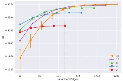
Figure 4.7 Augmented graphs:oc as a function of the number of added edges. Each entry is the average of 32 instances. Each series represents a different edge density for 200 vertices. . . 37
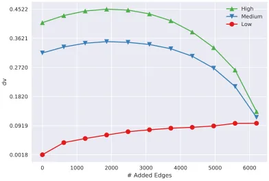
Figure 4.8 Augmented graphs: The final dv as a function of number of added edges. Each entry is the average of 32 instances. Each series represents a different degree distribution of the base bipartite graph. . . 38
Figure 4.9 Random graphs: How edge density relates to the oc and dv values. Each entry is the average of 32 instances. . . 40
Figure 4.10 An example of how funnels are likely to be found in geo-wrap instances. Suppose thatu is in a clique. Thenuv forms a funnel sinceN(u)−v is a clique. . . 41
Figure 4.11 An example of how unconfined vertices are found in Delaunay triangulation in-stances. If S = {v}, then |N(u)∩S| = 1 and N(u)−N[S] = ∅. Thus v is unconfined. . . 42
Figure 4.12 The MANN a3 instance. . . 45
Figure 4.15 Example of a small Hamming instance for binary vectors of length 3 and Ham-ming distance of 2. If we restrict the number of 1’s to 1 we get a Johnson graph (edges outlined in pink). . . 50 Figure 4.16 Examples of small coding-error instances. . . 50 Figure 4.17 Augmented graphs: Runtime as a function of oc value of using no reductions
(None), using LP (LP), using degree-one+dominance (DD), and using all re-ductions (All). Each entry is the average of 32 instances. The chart uses a log scale for the runtime. . . 54 Figure 4.18 Augmented graphs: Runtime ratio as a function of oc value of using LP (LP),
using degree-one+dominance (DD), and using all reductions (All) versus using no reductions. Each entry is the average of 32 instances. The chart uses a log scale for the runtime ratio. . . 55 Figure 4.19 Augmented graphs: Runtime and node ratio as a function of oc value of using
LP versus using no reductions. Each entry is the average of 32 instances. . . 55 Figure 4.20 Augmented graphs: Runtime and node ratio as a function of oc value of using
LP with degree-one+dominance versus using just degree-one+dominance. Each entry is the average of 32 instances. . . 56 Figure 4.21 Benchmark instances: Runtime and node ratio as a function of ocvalue of using
LP versus using no reductions. The charts use a log scale for the ratios. Each series represents different types of benchmarks: Hamming instances (Hamming), DIMACS based on random generators (Random), DIMACS based on hidden cliques (Clique), other DIMACS instances (Other), and coding-error instances (Coding Error). . . 57 Figure 4.22 Augmented graphs: Runtime ratio of using degree-one+dominance verses using
no reductions for different basedv. . . 61 Figure 4.23 Benchmark instances: Runtime ratio as a function ofdvof using degree-one+dominance
versus using no reductions. The chart uses a log scale for the runtime ratio and dv. Each series represents different types of benchmarks: DIMACS based on ran-dom generators (Random), DIMACS based on hidden cliques (Clique), other DIMACS instances (Other), and coding-error instances (Coding Error). . . . 62 Figure 4.24 A small 1dc example . . . 63 Figure 4.25 Augmented graphs: Runtime ratio as a function of edge density of using justLP
(LP), using degree-one+dominance (DD), and using all reductions (All) versus using no reductions. Each entry is the average of 32 instances. . . 65 Figure 4.26 Random graphs: Runtime ratio as a function of edge density of using just LP
(LP), using degree-one+dominance (DD), and using all reductions (All) versus using no reductions. Each entry is the average of 32 instances. . . 66 Figure 4.27 Geometric graphs: Runtime ratio as a function of edge density of using just LP
(LP), using degree-one+dominance (DD), and using all reductions (All) versus using no reductions. Each entry is the average of 32 instances. The chart uses a log scale for the runtime ratio. . . 67 Figure 4.28 Geo-wrap graphs: Runtime ratio as a function of edge density of using just LP
Chapter 1
Introduction
Given a graph G = (V, E), a vertex cover is a subset of V, C, such that for all uv ∈ E, at least one of u or v is in C. A minimum vertex cover is a vertex cover of the smallest possible size. Finding a minimum vertex cover for any graph is one of Karp’s [Kar72] original 21 NP-Complete problems. Over the years, many techniques and algorithms have been developed to solve this problem optimally with improved runtime. In 1977, Tarjan and Trojanowski [TT77]
introduced a branching based algorithm that computes the minimum vertex cover inO∗(1.2605n).1
Since then, a lot of work has been done to design techniques that reduces the problem instances to help improve the performance of branching algorithms; we call such techniques reduction rules. The goal of this thesis is to improve the performance of branching algorithms for finding minimum
vertex covers by using graph characteristics to identify which reductions will be most effective. The remainder of this chapter will formally define the minimum vertex cover and related problems,
provide a brief literature review on branching algorithms, highlight our main contributions, and
outline the rest of this thesis.
1.1
Terminology
For the rest of the thesis, we use the following terminology and notation: LetG= (V, E) be a graph. For any v ∈ V, we use N(v) to denote v’s neighbors, N[v] = N(v) +{v}, and deg(v) = |N(v)|.
If S ⊂ V, then N(S) = {v | u ∈ S and uv ∈ E} and N[S] = N(S) +S. We call N(X) the
neighborhood of X and N[X] the closed neighborhood of X. For two sets S and T, we useS\T to denote S minus T.
1
For the entirely of this thesis, we used modified big-Oh notation to suppress polynomially bound factors, i.e.,
1.2
Minimum Vertex Cover and Related Problems
TheMinimum Vertex Cover optimization problem is to find a smallest vertex cover for a given graph. More formally, given a graphG, what is the smallest numberksuch thatGhas a vertex cover
of sizek.Maximum Independent SetandMaximum Cliqueare two closely related optimization problems. A set S ⊂V is an independent set if for everyu, v ∈S,uv /∈E; aclique is a subset of vertices such that every pair of vertices in the clique are adjacent. TheMaximum Independent Set and Maximum Cliqueoptimization problems are to find the largest independent set/clique for a given graph. More formally, given a graph G, what is the largest k such that G has an
independent set/clique of size k. Note that for a graph G = (V, E) and its complement graph G, given a vertex coverC,S =V \C is an independent set andS is a clique ofG.
1.3
Branching Algorithms
Branching algorithms are commonly used to solve NP-complete problems. These types of algorithms use an exhaustive search with backtracking approach to recursively break a larger problem instance
into smaller sub-instances.
1.3.1 Generic Branching Algorithms for Minimum Vertex Cover
Algorithm 1 A branching algorithm for minimum vertex cover.
function Solve(I, C) . I: problem instance,C: current best solution value ProcessNode(I)
if LowerBound(I)≤C then .If the current lower bound is worse than C, do nothing
if IsSolved(I) then
if |I|< C then C← |I| end if end if
x←Select-Branching-Candidate(I) . Branch into smaller sub instances Cl←Solve(I\ {x}, C−1)
Cr ←Solve(I\N[x], C)
C ←min{C, Cl+ 1, Cr}
end if
return C . Return the size of the minimum vertex cover end function
Algorithm 1 shows the structure of a generic branching algorithm to find a minimum vertex cover
be easily modified to return an actual minimum cover.
Typically, branching algorithms first try to turn the problem instance into an easier instance (em-bodied by theProcessNodefunction), then branch into smaller sub-instances. One common flavor of branching algorithms is branch-and-bound (BB). In ordinary BB, the ProcessNode function does not modify the current instance. When theProcessNodefunction applies various reduction rules that shrink the problem instance we call the algorithms a branch-and-reduce (BR) algorithm.
For Minimum Vertex Cover a simple reduction rule involves vertices with degree 1: suppose that a vertex v only has u as a neighbor; then there will always be a minimum vertex cover that includes u but not v. Therefore, we can exclude v from the current cover while including u. The
first known BR algorithm was presented by Tarjan and Trojanowski [TT77]; their algorithm has a
time bound ofO∗(1.2604n).
In the context of branching and Minimum Vertex Cover, a simple branching candidate is a single vertex v, and the generated sub-instances either include or excludev. To improve runtime, branching algorithms typically utilize some sort of lower bound to prune the search space. For
Minimum Vertex Cover, a lower bound ` is a value with the property ` ≤ |C| for any vertex cover C; if the lower bound for instance I is greater than or equal to the current best solution, then the algorithm does not proceed to branch with I. A simple lower bound for a (sub-)instance
of Minimum Vertex Coveris the number of vertices minus one.
1.3.2 Measure and Conquer Analysis
Given the recursive nature of branching algorithms, it is difficult to perform detailed analysis to obtain tight complexity bounds. A simple measure, e.g., the number of vertices in a graph, can be
used to make the analysis easier. Improvements to complexity bounds for branching algorithms are then obtained by simplifying problem instances using long lists of new reduction and branching
rules.
Fominet al. [Fom09] are able to obtain improved bounds not by introducing new reduction rules, but by designing a sophisticated measure. Their reasoning is that a carefully designed, nonstandard
measure will be able to better exploit the recursive nature of branching algorithms. They
demon-strate the power of their technique by using a simple BR algorithm and comparing the bounds obtained from the analysis using a simple measure versus the analysis using a more complicated
measure. When they use the simple measure ofn=|V|, they obtain a time bound ofO∗(1.3250n),
which worse than Tarjan and Trojanowski’sO∗(1.2605n) algorithm. However, when they use a more sophisticated measure, they obtain an improved time bound of O∗(1.2201n). They dubbed their
Table 1.1Some results and key papers
Algorithm/Paper Complexity Notes
Fominet al., 2009 [Fom09] O∗(1.2201n) Introduced the measure and conquer Kneiset al., 2009 [Kne09] O∗(1.2132n)
Bourgeoiset al., 2012 [Bou12] O∗(1.2114n) Introduced the bottom up method
- O∗(1.0854n) For sparse graphs
Xiao and Nagamochi, 2013 [XN13] O∗(1.0836n) For sparse graphs Xiao and Nagamochi, 2017 [XN17] O∗(1.1996n)
1.3.3 Bottom-Up
Sparse graphs tend to be the harder instances to solve; this has motivated work to develop effective algorithms and techniques for sparse graphs. Additionally, many improvements for general graphs
can be obtained by carefully analyzing the sparse sub-instances. Unfortunately, the improvements
to the complexity bounds for solving Minimum Vertex Cover in sparse graphs do not always easily translate into improvements for general graphs. To address this, Bourgeois et al. [Bou12]
introduce thebottom-upmethod. The key idea of the bottom-up method is to design an algorithm for general instances by taking an algorithm for sparser instances and use branching methods to move from denser instances to sparser ones.
The bottom-up method works by essentially “propagating” any improvements from sparser graphs
to general graphs. This is accomplished by two features:
1. A good recursive measure (not unlike the measure and conquer method).
2. Good branching rules that allow denser graphs to be reduced effectively.
In the context of vertex cover, the algorithms designed with the bottom-up method take
algo-rithms/techniques designed for sparse graphs, then use well-designed branching rules to systemat-ically lower the density of general graphs. Bourgeois et al. [Bou12] demonstrate the effectiveness
of their bottom-up method by introducing an algorithm that solves Minimum Vertex Cover inO∗(1.2114n) (the best compared to other algorithms of the time). Xiao and Nagamochi [XN17]
utilize the bottom up method to great effect in their work in 2017, where they present an algorithm that solvesMinimum Vertex Coverfor general graphs inO∗(1.1996n); their algorithm is, to our knowledge, the fastest algorithm forMinimum Vertex Cover.
1.4
Summary and Outline
make it very difficult to implement these types of algorithms correctly. As a result, the practicality
of branching algorithms needs to be studied further. To this end, Akiba and Iwata [AI16] imple-ment a branching algorithm using techniques from Fominet al. [Fom09], Kneiset al.[Kne09], and
Xiaoet al.[XN13]. They show that their implementation is competitive with other state of the art
solvers forMinimum Vertex Cover. Despite the success of Akiba and Iwata, many questions still need to answered/addressed about the practicality of branching algorithms. Because each
branch-ing algorithm uses a different list of reduction and branchbranch-ing techniques, it is difficult to determine
how effective a specific technique is. In addition, branching algorithms typically apply reductions in a specific, fixed order; this is often done to simplify the analysis. For example, Xiao and
Nag-amochi [XN13] [XN17] always apply the funnel after the degree-one and dominance reductions in
order to simplify their analysis (see Sections 2.2 and 2.4 in Chapter 2 for descriptions of these reductions). This leads to the following questions for further study:
1. Does the order of reductions matter?
2. How do reductions interact with each other?
3. When is a specific reduction or branching technique useful to apply?
The answers to the above questions can lead to the design of better algorithms both from a the-oretical and practical aspect. To that end, the focus of this thesis is to address Question 3. To do
this, we made several modifications to Akiba and Iwata’s implementation to allow for more robust
experimentation. The remaining chapters go over the modifications and our experimental results. More specifically, Chapter 2 details the reduction rules implemented by Akiba and Iwata, Chapter
Chapter 2
Reduction Rules
In this chapter, we explain the details of the various reduction techniques used in branch-and-reduce algorithms for theMinimum Vertex Coverproblem. We say a reduction isdirectif the reduction does not introduce any new or auxiliary structures; conversely reductions that introduce additional
structures are calledindirect reductions.
2.1
Definitions and Terminology
Definition 1 (Dominance). We say a vertexv dominates a vertex uifN[u]⊂N[v].
Definition 2 (Child and Parent). ForS⊂V,u∈N(S) is achild of S if it has a unique neighbor s∈S, i.e., |N(u)∩S|= 1, called its parent.
Definition 3 (Contracting a set S). Given a graph G and an S ⊂ V, we can contract S by removing all vertices of S and introducing a new vertexs such that a vertex u6∈S is adjacent to sifu is adjacent to a vertex inS.
Definition 4 (Cut/s-t cut). For a graph G= (V, E), a cut S is a partition of V. An s-t cut is a cut such that vertexsis contained in S and vertex tis contained in V −S.
2.2
Unconfined vertices
We begin with some common reduction rules:
1. Degree-one: If deg(v) = 1 for v ∈ G, there exists a minimum vertex cover of G that does not includev (and must includev’s only neighbor).
2. Dominance: If vertex v dominates another vertex, there exists a minimum vertex cover that contains v. If v has a degree-one neighborw,v dominatesw. Therefore, the dominance
Xiao and Nagamochi [XN13] introduce a generalization of dominance. They observe that the
fol-lowing lemma can be used to determine whether a vertexv should be included in the cover:
Lemma 1. LetS be an independent set and suppose that for any minimum vertex coverC,S∩C= ∅. Then for all childrenu∈N(S), there is at least one vertexw∈N(u)−N[S]that is not contained
in any minimum vertex cover of G.
Proof. We can prove Lemma 1 by obtaining a contradiction. Let S be an independent set such
that there is no minimum vertex coverC such thatS∩C=∅. Suppose that there is a child ofS, u ∈N(S) such that all w ∈N(u)−N[S] are contained in every minimum vertex cover. Let p(u)
be u’s parent. Let C be a minimum vertex cover. All of u’s neighbors exceptp(u) are in C. Since
p(u) is not inC, u must be. LetC0 =C− {u}+{p(u)}.C0 is also a minimum vertex cover. This is a contradiction since p(u)∈S.
Xiao and Nagamochi argue that ifS ={v}, and there is a childu∈N(S) such thatN(u)−N[S] =∅,
the assumption of Lemma 1 is false, i.e., there is a minimum vertex cover that contains S, and we
can includev in the cover.
Algorithm 2 ComputeConfiningSet(v) Require: Some vertexv
Ensure: Sv is the confining set of v
Sv ← ∅
W ← {v}
while W is non-empty do .Loop Invariant: Sv is not contained in any cover
forall unique children (u) of Sv do
if |N(u)−N[Sv]|= 1 then
w←N(u)−N[Sv]
W ←W ∪ {w}
else if |N(u)−N[Sv]|= 0 then
return ∅ end if end for
if W is notan independent setthen return ∅
end if Sv ←Sv∪W
end while return Sv
They use this observation to develop Algorithm 2. If Algorithm 2 returns an empty set, we say that
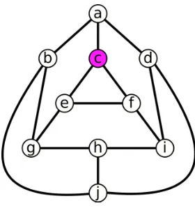
Figure 2.1 Vertexcis confined bySc={c, g, i}
As an example, consider Figure 2.1. If we start with S = {c}, N[S] = {a, c, e, f} and a, e, and f
arec’s children.N(e)−N[S] ={g} andN(f)−N[S] ={i}, so after the first iteration,g andiare
added toS. The algorithm then terminates and returns S since there are no more valid children of S in the graph. Because S ={c, g, i} 6=∅,c is confined and cannot be reduced by the algorithm.
We note that if v dominates u,v is unconfined since N(u)−N[S] =∅. To illustrate this, suppose
that a vertex v dominates u and N(u) = {a, b, c, v}. Starting with S = {v}, when Algorithm 2 evaluates u,N(u)−N[S] =N(u)−N[v] =∅. Therefore, Sv =∅ and v is unconfined.
The degree-one, dominance, and unconfined reductions are all direct reductions.
2.3
Folding
Now we focus on reductions that are based on contracting sets. One simple reduction is the
fold-2 reduction. The fold-2 reduction is used in many algorithms and is based on the following lemma [F¨ur06] [Fom09] [Kne09] [Bou12] [XN13] [XN17]:
Lemma 2. If v is a vertex with deg(v) = 2 and non-adjacent neighbors, let G0 be a graph obtained from G by contracting N[v] to a new vertex w. For any minimum vertex cover, C0, of G0, the
followingC is a minimum vertex cover of G:
C= (
C0∪ {v} w /∈C0 (C0− {w})∪N(v) w∈C0
) .
Since its introduction, there have been two different generalizations of the fold-2 reduction: folding
completek-independent sets, and Fomin folding.
2.3.1 Complete k-Independent Sets
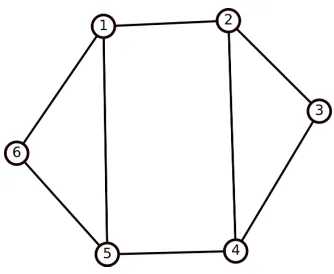
Figure 2.2 Example of a twin (note that no vertex is unconfined).
Definition 5 (k-independent set). We say a set A ={v1, ..., vk} of unique vertices is a complete
k-independent set, ifN(v1) =...=N(vk) and deg(v1) =k+ 1.
The fold-2 reduction is the special case where k = 1. When k = 2, we call the two vertices in
A={v1, v2}twins. In this situation,v1 is a twin ofv2 and vice-versa.
As an example, consider Figure 2.2: a and b share the same neighbors and are both degree 3;
therefore aand bare twins. Verticesiand j are also twins for similar reasons.
Using Lemma 2 as a base and the definition ofk-independent set, Xiao and Nagamochi generalize fold-2 into the following reduction:
Lemma 3. Let A ⊂V be a k-independent set. If N(A) is an independent set, then let G0 be the graph formed by contracting N[A] to a new vertexw. Then for any minimum vertex cover, C0, of
G0, the following cover C is a minimum vertex cover of G:
C = (
C0∪A w /∈C0
(C0− {w})∪N(A) w∈C0
Moreover, if N(A) is not an independent set, letG0 be the graph formed fromGby removing N[A]. If C0 is a minimum vertex cover for G0, then C0∪N[A]is a minimum vertex cover of G.
2.3.2 Fomin Folding
Fomin et al. [Fom09] generalize the fold-2 reduction by introducing the Fomin folding technique. A vertexv is considered foldable if for all U ={ui, uj, uk} ⊂N(v), i6=j6=k, there is at least one edge contained in U. To Fomin fold a vertex v is to create a new instance G0 using the following procedure:
1. Add a new vertex uij for each non-adjacent pair ui, uj ∈N(v)
2. Add edges uijx wherex∈N(ui)∪N(uj)
(a) Before foldingv
(b) After foldingv
Figure 2.3 Example of folding a vertexv
4. RemoveN[v]
Figure 2.3 illustrates the result of Fomin folding a vertex. For vertexv there are 3 possible values
forU :{1,2,3},{1,2,4},{2,3,4}. In all three cases, there is an edge contained in U. Therefore,v
is a foldable vertex. To create the folded instance, after removing vertices v, 1, 2, 3, and 4, new vertices 13 and 14 are added since 1 is not adjacent to either 3 or 4; vertices 23 and 24 are added
for the same reason. Then edges such as {13,5} and {13,8} (blue edges) are added since, in the
original graph, vertex 5 is adjacent to vertex 1 and vertex 8 is adjacent to vertex 3. The red edges are added to connect all new vertices to each other.
From the folding procedure above, Fominet al. introduce the following reduction:
Lemma 4. If v is a foldable vertex, let G0 be a graph obtained from Gby Fomin folding v. Let C0 be a minimum vertex cover of G0 and U ={uij|uij ∈C0 |}, then following C is a minimum vertex
cover of G:
C = (
(C0−U)∪N(v) ∀uij ∈G0, uij ∈C0
(C0−U)∪(N[v]− {ui, uj}) ∃!uij, uij ∈/ C0 )
.
2.4
Alternative Structures
In addition tok-independent sets, Xiao and Nagamochi [XN13] also introduce the notion of
alter-native structures:
Definition 6 (Alternative). For a graph G = (V, E), A and B ⊂ V are called alternative if |A|=|B| ≥1 and there exists a minimum vertex cover C such thatC∩(A∪B) =AorB.
Let A and B be an alternative of G and let G0 be the graph formed from G by removing A∪ B ∪(N(A)∩N(B)) and adding an edge ab for each pair of nonadjacent vertices a, b with a ∈
N(A)−N[B],b∈N(B)−N[A]. A reduction based on alternatives works as follows:
(a) sort funnel (b) a non-short funnel
Figure 2.4 ais a funnel in both examples
Figure 2.5 A desk
cover C is a minimum vertex cover of G:
C= (
C0∪(N(A)∩N(B))∪A (N(B)−N[A])⊂C0
C0∪(N(A)∩N(B))∪B (N(A)−N[B])⊂C0
Xiao and Nagamochi define the following alternatives:
Definition 7 (Funnel). A vertex aandN(a) is called a funnel if for some b∈N(a),N[a]−bis a clique. In this case,A={a}andB ={b}is an alternative. A funnel is calledshortifN(a)∩N(b) =∅ and there are at mostdeg(b) pairs of nonadjacent vertices betweenN(b)−aand N(a)−b.
Definition 8 (Desk). A chord-less 4-cycle,u1u2u3u4, where the degree of each vertex is at least 3
is a desk if the setsA={u1, u3}andB ={u2, u4}have no common neighbors and|N(A)−B| ≤2
and |N(B)−A| ≤2.
Figure 2.4 shows an example of two funnels, one short the other not. In Figure 2.4a, A={a} and B = {b} are a short funnel since there are only two edges missing between the neighborhoods.
However, in Figure 2.4b, removing the edge ec turns A and B into a non-short funnel since then
B = {b, d}, we see that |N(A)−B| = 2 (the vertices outlined with red) and |N(B)−A| = 2
(vertices outlined in blue).
2.5
LP Reduction
This reduction is based on theLPrelaxation of theMinimum Vertex Coverproblem. Many NP-Complete problems have an equivalent (binary) integer linear programming (ILP) formulation. ForMinimum Vertex Cover, the formulation can be stated as:
minimize P v∈V
xv
s.t. xu+xv ≥1 foruv ∈E
xv∈ {0,1} forv∈V
Ifxu= 1, then u is in the cover while if xu = 0 thenu is not in the cover.
2.5.1 LP Relaxation
The LP relaxation is the same as the ILP formulation except the constraint that xv ∈ {0,1} is replaced with xv ≥0. Nemhauser and Trotter [NT75] show that for the aboveLP, there exists an optimal solution such that each variable takes a value of 0, 1, or 12. Additionally, they show that
if a variable xv takes an integer value in an optimal LP solution, there exists an optimal integer solution with the same value for xv.
Given a graphG, an optimal solution to theLPcan be computed by finding the maximum matching for the associated LR-graph. TheLR-graphfor a graph G= (V, E) is a bipartite graphG0 = (V0= LV ∪RV, E0) such that
• LV ={lv |v∈V}
• RV ={rv |v∈V}
• E0 ={lurv |uv ∈E} ∪ {lvru|uv ∈E}
LetC0 be a minimum vertex cover of the bipartite G0 (which can be computed in polynomial time from a maximum matching ofG0). Then the value ofxv in the optimalLP solution for vertexv, is:
xv =
0 lv, rv 6∈C0
1 lv, rv ∈C0
1
2 otherwise
The LPreduction uses the solution values to include or exclude vertices from the cover: if xv = 1,
2.5.2 Extreme optimal solutions
Iwataet al.[Iwa14] introduce a way of minimizing the number of 12 values in theLPsolution. They accomplish this by turning the LR-graph, G0, into a flow network by adding vertices s and t (the
source and sink respectively) and edges {sl|l∈LV} ∪ {rt|r ∈ RV}. A capacity of 1 is used for all edges and all edges are directed such that flow can only pass fromstoLV, fromLV toRV, and
fromRV tot. Note that for a flow network, a cut is minimum if the sum of flow through the edges
connecting the partitions is minimum and that an s-t cut typically involves the source (s) and the sink (t); we call a s-t cut S for the flow graph of G0 normalized if for each v ∈ V, S contains at most one of lv and rv. After computing the maximum flow, given some normalized minimum s-t
cut, S, then the newLP solution value for vertex v,xv, is given by:
xv =
0 lv ∈S, rv 6∈S 1 lv 6∈S, rv ∈S
1
2 otherwise
An extreme minimum cut is a normalized minimum cutS such that there is no other normalized minimum cut T such that S ⊂T. Iwata et al. [Iwa14] show that if you use an extreme minimum cut, the number of fractional values in the newLPsolution is minimized; they called such a solution an extreme optimal solution.
Algorithm 3 ComputeExtremeOptimalSolution(G0)
Require: G0 = (LV, RV, E) an LR-graph transformed into a flow network
Ensure: x∗ is the extreme optimal solution vector
GR←ComputeMaximumFlow(G0) . GRis the residual graph
SCC ←GetStronglyConnectedComponents(GR)
S ← {s}
while ∃valid T ∈SCC do .Compute an extreme minimum s-t cut, S if N+(T)⊂S and IsNormalized(S∪T)then
S ←S∪T
SCC ←SCC−T break end if
end while
x∗←GetLPSolution(S) . Assign 0,1, or 12
return x∗
2.5.3 Lower bounds
Iwata et al. [Iwa14] show that we can use the sum of the values of an extreme optimal solution to obtain anLP based lower bound for the size of a minimum vertex cover. Akiba and Iwata [AI16] later demonstrate that we can use the maximum matching of the LR-graph to compute a cycle cover based lower bound. For a graph, a set of vertex-disjoint cycles,{C1, . . . , Ck}, is a cycle cover if each vertex is contained in one of the cycles. Given a cycle cover,{C1, . . . , Ck},Pki=1
l|C
i| 2
m is a
lower bound for the size of a minimum vertex cover. Similarly, we can use clique covers to compute another lower bound. For a graphG= (V, E), aclique cover is a set of disjoint cliquesC1, . . . , Ckif each vertex is contained in one of the cliques. For any clique coverC1, . . . , Ck,
k P
i=1
(|Ci|−1) =|V|−k
gives a lower bound for the size of the minimum vertex cover. Chapter 3 explains the specifics on how these lower bounds are computed.
2.6
Concluding Remarks
In this chapter, we looked at a variety of different reductions used by branch-and-reduce algorithms
Chapter 3
Implementation Details
Akiba and Iwata implemented (vcsolver), a branch-and-reduce solver for the Minimum Vertex Coverproblem. While vcsolveris competitive with industrial-strength solvers such as CPLEX, it is difficult to isolate the effectiveness of specific reductions using their software because the
re-ductions are applied in nested groups. For example, it is not possible to apply the LP reduction only: the degree-one, dominance, and fold-2 reductions are automatically applied as well. We
mod-ifiedvcsolverto be easier to read and understand. In addition, we added some new features that improve our ability to use the software in our experiments: the modified solver can apply specific reductions individually and can provide much more detailed tracing and debugging messages. The
rest of this chapter will focus on implementation details of vcsolverand the modifications made.1
3.1
Implementation Overview
All branching algorithms involve recursively solving sub-instances; forMinimum Vertex Cover, a sub-instance is a subgraph of the original graph.vcsolver uses the original graph and a status vector to represent sub-instances. A vertex can have one of the following statuses:included/excluded means that the vertex is in/not in the vertex cover; folded means that the vertex is temporarily removed due to folding ak-independent set or an alternative structure (refer to Chapter 2 for more details) or other reasons; and undecided means the vertex is part of the current sub-instance. A status vector is an array that contains the integer representations of the status of each vertex; included and excluded are represented by 1 and 0 respectively, folded is represented by 2, and undecided is represented by -1. The value of a status vector is given by the number of included
vertices. vcsolveruses a status vector, denoted as theoptimal status vector, to keep track of the current best cover. The value of the optimal status vector, denoted by optimal_value, is used as the global upper bound (GUB) during the computation.
1
The modified software, along with various scripts and our own C++ solver, is available at
Algorithm 4 ProcessNode(I)
n←# of vertices in the graph
undecided←# of undecided vertices Reduce(I)
if LowerBound(I)≥optimal value then . optimal valueis the global upper bound
node status← lower bound cut return
end if
if undecided== 0 then .Iis solved so the optimal value is updated
optimal value←min(current value,optimal value)
Reverse() .Reverse effects of folded structures/alternatives
node status← solved return
end if
node status ← alive
if Inotconnected orundecided is smallthen
Component-Solve(I) . Create and solve smaller sub-instances and combine results else
Branch(I) . Select and branch on branching candidate
end if
Algorithm 5 Branch(I)
b←branching candidate . bis a vertex with maximum degree
M[b]←Mirrors(b) .Check if bhas any mirrors
if |M[b]|>0then . Perform a left branch
Solve(I, include band M[b]) else
Solve(I, include b) end if
A node contains a status vector and a node status. In general, a node status denotes the state of a node with respect to the search space. A node can have one of the following statuses (each will be explained later): lb_cut,solved,alive, andred_cut.
The main implementation challenges of any branching based algorithm are the ProcessNode function, from Algorithm 1 in Chapter 1, and the branching process. Algorithms 4 and 5 provide a high level overview of howvcsolverimplementsProcessNodeand the branching process. When vcsolverprocesses a node, it first applies reduction rules. Then it computes a lower bound, using only the current node, and compares it to the GUB. If the lower bound is larger,vcsolver prunes the current branch and updates the current node’s status tolb_cut. Otherwise, if the node’s status
vector contains only 1’s and 0’s, the node’s status is set to solved. If there are still undecided or
folded vertices, then the node’s branch is still alive and the node’s status is set toalive. From here
vcsolver branches on the current node (see Algorithm 5). To improve the runtime, if the graph is disconnected or the number of undecided and folded vertices is small, vcsolver recursively solves each smaller sub-instance individually (illustrated by the Component-Solve function in Algorithm 4). If Component-Solveis called because the number of undecided and folded vertices is small, then the node’s status is set tored_cut.
3.1.1 Reductions
Algorithm 6 Reduce(I)
Each reduction function returnsTrue if at least one vertex is reduced, Falseotherwise
n←# of vertices in the graph
undecided←# of undecided vertices while undecided>0 do
if degree-one(I) thencontinue
if n∗SHRINK≥undecidedthen . The instance is reduced to a small enough size
Component-Solve(I) .Apply the solver to the smaller instance
node status ← reduction cut end if
if dominance(I) thencontinue if unconfined(I) thencontinue if lp(I)then continue
if packing(I) thencontinue if fold2(I)then continue if twin(I) then continue if funnel(I) then continue if desk(I) thencontinue break
Table 3.1Time complexity for the reductions presented.
Reduction Complexity
degree-one O(n)
dominance O(n3)
unconfined O(n4)
LP (Initial) O(m
√ n) LP (Update) O(m+n)
fold-2 O(m)
twin O(m)
desk O(m)
funnel O(mn)
Implementing reductions is a big challenge to developing branch-and-reduce based solvers. Because the degree-one, dominance, and unconfined reductions are straightforward to implement we focus
on the other reduction implemented byvcsolver.
There are two components to theLP reduction: 1) computing the maximum matching of the LR-graph, and 2) computing the extreme optimal solution. It is known that a maximum matching for
a bipartite graph translates into a maximum flow and vice versa [JF62]. Note that in Chapter 2,
we introduced the LP reduction in the context of computing a maximum flow; in this chapter we instead talk about computing maximum matchings. The maximum matching is computed using
the Hopcroft-Karp [HK73] algorithm and the extreme optimal solution is calculated as described in Algorithm 3 from Chapter 2. To improve the performance of LP reduction, the LR-graph and corresponding matching are not calculated from scratch each time the reduction is invoked. Instead,
vcsolver uses the linear-time update method described by Iwataet al. [Iwa14].
Since the fold-2 and twin reductions are only concerned with vertices that have degree 2 and 3 respectively, it takes constant time to check if a vertex is foldable or part of a twin. Therefore, for
these two reductions, the main time overhead comes from computing the degree of every vertex. In
vcsolver, the degree of any vertex v is the number of neighbors u such that the u is undecided. Ifv hasdneighbors, it takesO(d) time to calculatev’s degree and takesO(m) time in total where
m is the total number of edges.
Similarly, since the desk reduction can only be applied to vertices that have degree 3 or 4, it takes constant time to check if a vertex is a part of a desk (see Chapter 2 for more details).
However, a funnel reduction is more difficult to detect than a desk. Given a vertexv, vcsolver attempts to find more than oneu∈N(v) such that|N(v)∩N(u)|<|N(v)| −1; if there is only one
u, then vu forms a funnel. If v and u have dv and du neighbors respectively and the vertices are
sorted by degree, computing |N(v)∩N(u)| takes min({du, dv}) time. Therefore, it takes O(dvS) where S = P
u∈N(v)
min({du, dv})) time to process v and takes O(mn) time in total where m is the
In vcsolver, the reductions are applied in the following sequence: 1) degree-one, 2) dominance, 3) unconfined, 4)LP, 5) packing, 6) fold-2, 7) twin, 8) funnel, and lastly, 9) desk. Since the graph changes each time a vertex is reduced, the sequence of the reductions is restarted whenever any
reduction reduces at least one vertex. For example, if the degree-one, dominance, and unconfined
reductions do not reduce any vertex but theLPreduction does, then the sequence is restarted and vcsolver attempts the degree-one reduction again before attempting other reductions. Table 3.1 gives a summary of the worst-case, i.e., no vertex is reduced, runtime complexity of a single call of
an individual reduction.
In the original implementation of vcsolver reductions are split into the following groups – Group 0: degree-one+dominance+fold-2,
Group 1:LP,
Group 2: unconfined+twin+funnel+desk, and
Group 3: packing.
Selecting reductions from group iwill cause reductions belonging to groups 0, . . . , i to be applied,
i.e., there is no way to apply individual reductions selectively. In our version of vcsolver, we separate the reductions into independent options, and all reductions can be applied independently from one another.
3.1.2 Lower Bounds
vcsolveruses 4 different lower bound computations: 1) value of the current node’s status vector; 2) clique cover based; 3)LP based; 4) cycle cover based.
Recall that a clique/cycle cover is a collection of disjoint cliques/cycles such that each vertex is
contained in exactly one clique/cycle.
vcsolver computes a clique cover in linear time using a greedy algorithm. For a graph, let C = {C1, . . . , Ck} be the set of all known cliques, andC[v] denote the clique that contains v. For each
vertex v, let Pi ={u|u∈N(v) andu∈Ci}. If there is a nonemptyPi such that |Pi|=|Ci|, then we can add v to Ci; if there are multiple such Pi’s, we pick the one of the largest size; If there
are none, we create a new clique{v}and add it toC. Invcsolver’s implementation of the clique cover, it takes constant time determine the size of a clique and which clique a vertex belongs to. Therefore, since it takesO(|N(v)|) time to process a vertexv, it takes linear time overall.
For anLP based lower bound, Iwataet al. [Iwa14] show that the sum of the values of an extreme optimal solution of theLP relaxation is a lower bound for Minimum Vertex Cover.vcsolver uses the current status vector as the extreme optimal solution: vertices that are folded are ignored
while undecided vertices are treated as having a 12 value.
Akiba and Iwata show that it is possible to use the extreme optimal solution of theLP relaxation to obtain a cycle cover. In this context, we consider a single edge a cycle of length two, but do not
Figure 3.1 Example of how to split a cycle: 1,2,3,4,5,6 is a part of a cycle cover. After splitting, the cycle cover now includes 1,5,6 and 2,3,4.
{uv | lurv ∈ M} is a cycle cover of the original graph. However, if M is not a perfect matching,
there will be single vertices not covered. In this situation, vcsolver ignores these single vertices. Additionally, vcsolver improves the cycle cover lower bound by splitting even length cycles into two smaller odd length cycles. Specifically, supposev1, . . . , vl is an even length cycle with at least 6 vertices. If there are four vertices, vi, vi+1, vj, vj+1, where 1≤i, j ≤l, andvivj+1 and vjvi+1 are
edges, we can split v1, . . . , vl into two smaller odd length cycles.
Figure 3.1 provides an example of how to split a cycle.
For any even-length cycle C=v1, . . . , vL of lengthL≥6,vcsolver identifies the vertices to split on in the following way: For a vertex vi ∈ C, let S be the set of vi’s neighbors that are also on
the cycle. If there is a vk∈S such thatvk−1 ∈N(vi+1), thenvcsolver uses vi, vi+1, vk−1, andvk to split C. For vcsolver, the main bottleneck comes from checking the neighbors of each vertex in the cycle; therefore it takes O(Ldmax) time where dmax = max(|N(v)|, v ∈C) and in the worst
case,O(n2) time in total.
3.1.3 Branching
The most basic branching method forMinimum Vertex Cover is to choose a vertex and create two subinstances: one where the vertex is included and one where it is excluded. By default,
vcsolver picks a vertex with maximum degree, and, in case of a tie, picks a vertex that also minimizes the number of edges among its neighbors. In addition to maximum degree branching,
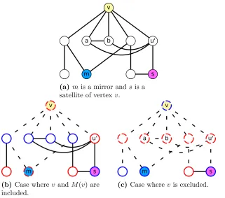
vcsolveralso utilizes Fominet al.’s [Fom09] mirror branching rule to improve the runtime. Given a vertexv, amirror ofv is a vertexu∈N2(v) such thatN(v)−N(u) is a clique. LetM(v) denotes
the set of all mirrors forv. If|M(v)|>0, if we branch onv, we can also includeM(v) in the cover
when we includev.
Figure 3.2a illustrates an example of a mirror of v:m is a mirror since a, b, and u0 form a clique.
(a)mis a mirror andsis a
satellite of vertexv.
(b) Case wherev andM(v) are
included.
(c) Case wherev is excluded.
Figure 3.2 Example of a mirror and mirror branching.
reading the input graph... n = 62, m = 264
opt = 46, time = 0.003
Figure 3.3 Example output of vcsolver.
3.2
Tracing and Instrumentation
The originalvcsolver provides minimal output information: the number of vertices, the number of edges, the size of the minimum vertex cover, and the total runtime (see Figure 3.3). We modified
vcsolver to output more information such as (i) the status vector — so that the cover can be independently verified and displayed; (ii) the runtime devoted to specific parts — so that efficiency of reductions can be measured; (iii) the number of vertices reduced by a specific reduction; and
other useful information. Figures 3.4 and 3.5 show an example of the output format of our version
of vcsolver.
The original vcsolver’s --debug option provides information such as the number of undecided vertices before and after a reduction is applied, the number of mirrors a branching candidate has,
etc. We enhanced vcsolver’s debug capabilities by including a runtime trace option (--trace) that displays important runtime information such as the current state of the branch-and-reduce
algorithm, the selected branching candidate, and important information about the current node.
Table 3.2Summary of runtime options available in our enhanced vcsolver.
Short Long Arguments Description Default Value
-l --lb 1 (int) Determines the method used to
com-pute the lower bound.
0
0: the value of the current status vector, 1: clique cover based, 2: LP based, 3: cycle cover base, 4: compute each and use the best
-b --branching 1 (int) Determines which branching method to use
2
0: random selection, 1: minimum de-gree, 2: maximum degree
-t --timeout 1 (int) Sets the timeout limit in seconds 3600 --root 0 Only process the root node – --deg1 0 Enable the degree-one reduction – --dom 0 Enable the dominance reduction – --fold2 0 Enable the fold-2 reduction –
--LP 0 Enable the LPreduction –
--unconfined 0 Enable the unconfined reduction – --twin 0 Enable the twin reduction – --funnel 0 Enable the funnel reduction – --desk 0 Enable the desk reduction – --packing 0 Enable the packing reduction – --trace∗ 1 (int) Enables levels of runtime tracing 0
0: no trace, 1: short version, 2: includes status vectors
--disabled∗ 0 Disable ineffective reductions after the root
–
--tiered_disabled∗ 0 Disable ineffective indirect reductions after the root
–
--size∗ 1 (float) Change the size threshold that deter-mines when to apply reductions
1.00
-d --debug 1 (int) Enables various levels of debug mes-sages
0
0: no debug, 1: basic branching, 2: de-tailed branching and basic reduction, 3: detailed reduction
The Arguments column denotes the number of arguments (and type) the option requires, a ∗
InputFile ../instances/snap/keller4.txt
Options --deg1 --dom --fold2 --LP --unconfined --twin --desk --funnel --packing -l4 num_vertices 171 num_edges 5100 value 160 runtime 3.901 num_nodes 8152 ...
Figure 3.4 Example of the basic statistics our modified version reports.
... lpTime 0.451 domTime 0.382 degTime 0.019 foldTime 0.019 Vertices Reduced: degree1 13538 dominance 17248 unconfined 26255 lp 10993 packing 5822 fold2 2738 twin 77 funnel 132 desk 72 ...
Figure 3.5 Example of the some of the additional statistics our modified version reports.
and which branch is currently being processed; and level 2 adds the current status vector and the
current node status. Our intent is to make it easier for users to follow along with the branching
nature of the computation.
Figure 3.6 provides a snapshot of the level 1 trace option output. For each node, the trace reports
the label, the optimal value (GUB, i.e. the global upper bound), the lower bound (LB), the number
of remaining undecided vertices (n), the status, and the value of the current status vector. Each node can have one of the following labels:RTdenoting the node is the root, 1denotes the node is a
left branch, and 0denotes the node is a right branch. If Component-Solveis applied to a node, acis added to its label. Whenever the current branching candidate is printed, a∗denotes that the integer printed is the vertex id from the input file rather than the id used internally invcsolver; vcsolver sorts and labels vertices based on their degree, rather than the input order, to reduce the time needed to find a branching candidate when using maximum degree branching. A $ next
GUBdenotes that the upper bound at the node improved on the global one.
For a level 2 trace, the current status of each vertex is printed just before the value of the current status vector. Figure 3.7 shows what the output of a level 2 trace can look like. A “_” indicates an
unused vertex, e.g., when the graph’s source file uses non-contiguous vertex numbers, a 0indicates
...
= 0c GUB: 46 , LB: 45, n = 18, - alive | 37 RT c GUB: 9 $, LB: 4, n = 9, - alive | 0
/\ branching_vertex: * 1
= 1c GUB: 5 $, LB: 5, n = 0, = solved | 5 __ left_branch_done: * 1
^^ right_branch: * 1
= 0c GUB: 5 , LB: 5, n = 0, / lb_cut | 5 _ right_branch_done: * 1
RT c GUB: 4 $, LB: 4, n = 9, / lb_cut | 0 _ right_branch_done: * 2
__ left_branch_done: * 1 ^^ right_branch: * 1
= 0c GUB: 46 , LB: 44, n = 43, - alive | 23 /\ branching_vertex: * 3
= 1c GUB: 46 , LB: 45, n = 29, - alive | 31 /\ branching_vertex: * 4
= 1c GUB: 46 , LB: 46, n = 9, / lb_cut | 42 __ left_branch_done: * 4
^^ right_branch: * 4
= 0c GUB: 46 , LB: 47, n = 0, / lb_cut | 47 _ right_branch_done: * 4
__ left_branch_done: * 3 ^^ right_branch: * 3
= 0c GUB: 46 , LB: 47, n = 0, / lb_cut | 47 _ right_branch_done: * 3
_ right_branch_done: * 1
= 0c GUB: 114 , LB: 104, n = 79, red_cut | 68 _ right_branch_done: * 13
__ left_branch_done: * 4 ^^ right_branch: * 4
= 0c GUB: 114 , LB: 105, n = 90, - alive | 61 /\ branching_vertex: * 7
...
Figure 3.6 Example trace output.
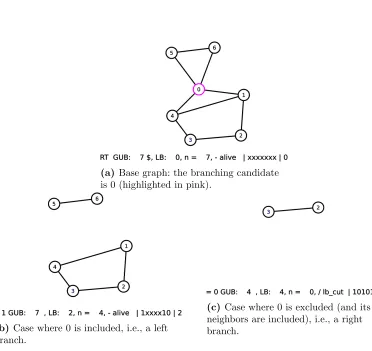
= 1c GUB: 12, LB: 8, n = 7, - alive | __---1-1-x----xx-1x--xx1---x01---1-- | 5
(a)Base graph: the branching candidate is 0 (highlighted in pink).
(b) Case where 0 is included, i.e., a left
branch.
(c) Case where 0 is excluded (and its
neighbors are included), i.e., a right branch.
the vertex is undecided, and a-indicates that the vertex is not currently relevant, e.g., it belongs
to a component other than the one being solved at the current node.
Figure 3.8 shows an example of what the trace would look like when applied to a graph. In this
example, only the degree-one reduction is applied. The root instances and the associated trace is
in Figure 3.8a; all vertices are undecided. The left branch, i.e., the case where we include vertex 0, is illustrated in Figure 3.8b. Here only vertices 5 and 6 are reduced so the status vector has xfor
vertices 1, 2, 3, and 4. In the right branch, Figure 3.8c, although the graph is reduced by
degree-one, the value is not better than the current optimal value (obtained from other nodes of the left branch) so the node’s status is set to lb_cut.
3.3
Concluding Remarks
In this chapter, we went over the key implementation details of Akiba and Iwata’s vcsolver. Additionally, we introduced our enhancements and modifications tovcsolverthat allow for more robust experimentation.
Our three main enhancements were: 1) the separation of reductions, 2) additional runtime statistics
reported, and 3) a runtime trace. In our modified vcsolver, as opposed to grouping reductions together, each reduction is given its own option and can be used independently from one another. Our modified version also reports additional statistics such as the total runtime of each reduction
and the number of times a reduction is called. Lastly, we enhanced vcsolver’s debugging capa-bilities by including a trace option that makes it easier to follow along with the branching nature of the algorithm. Table 3.2 provides a summary of the runtime options available in our enhanced
vcsolver.
Chapter 4
Graph Characteristics
Many reduction rules have been proposed to improve the theoretical effectiveness of branch-and-reduce (BR) algorithms for Minimum Vertex Cover. Akiba and Iwata’s [AI16] vcsolver im-plements several of these, and they demonstrate, experimentally, that the runtime of BR algorithm
implementations can be competitive with industrial optimization software such as CPLEX [Cpl].
Our premise is that, while doing all reductions can greatly improve the performance of a BR
algorithm, there are circumstances where using a targeted subset of reductions is more effective in
practice. More specifically, since most of the reductions have quadratic or cubic time complexity, ineffective reductions will unnecessarily add to the overall runtime. To evaluate the effectiveness of
specific reductions in isolation, we made modifications tovcsolverso that it is able to apply each type of reduction independent of the others. Our modifications and enhancements are detailed in Chapter 3.
In this chapter, we focus on how graph characteristics relate to the effectiveness of reductions. This chapter is broken up into three sections: the first section goes over measures and characteristics
and how they relate to the effectiveness of reductions; the second section introduces the graph
classes used in our experiments; additionally, this section highlights interesting characteristics for each graph class; the last section presents our experimental results.
4.1
Measures and Characteristics
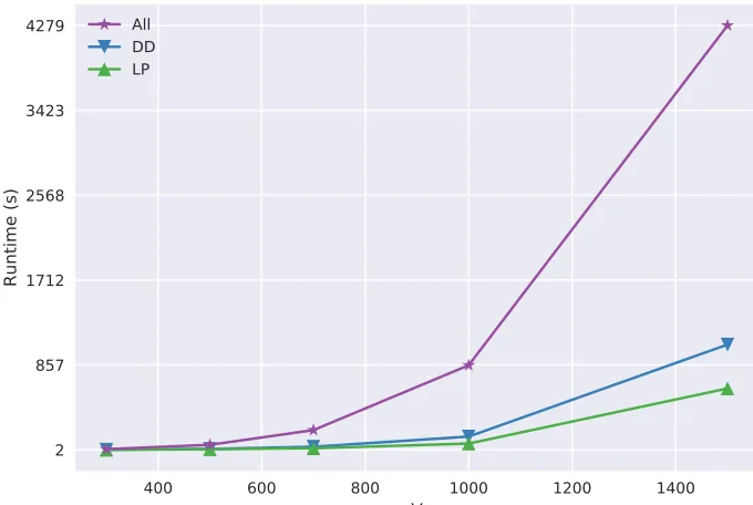
Figure 4.1 shows, for a specific class of graphs, the relative effectiveness of using all reductions (degree-one, dominance, fold-2,LP, unconfined, twin, funnel, desk, packing) versus using just the degree-one+dominance reductions (dd) or using just theLPreduction (lp). We can see that using more reductions does not necessarily give lower runtimes. It is clear that the performance of BR
algorithms can be improved by being more selective about which reductions to apply. However,
400 600 800 1000 1200 1400
V
2 857 1712 2568 3423 4279
Runtime (s)
All DD LP
Figure 4.1 phat-1 series: Runtime as a function of the number of vertices. The reductions presented are:
the degree-one+dominance reductions (DD), theLP reduction (LP), and all reductions (All). From this,
it is obvious that using all reductions does not always lead to better runtimes.
The rest of the section introduces the graph characteristics and graph classes that are the focus of our experiments.
4.1.1 Odd Cycles
In this section, we discuss the relationship between the number of disjoint odd cycles in a graph and the runtime performance of the LP reduction. Since a linear program for Minimum Vertex Cover gives all-integer solutions when applied to bipartite graphs, our intuition suggests that a linear program would also give all-integer (or almost all-integer) solutions when applied to graphs that become bipartite after a small number of edges removed.
To further explain this, suppose we have a graph G = (V1, V2, EX, EB), where vw ∈EB if v ∈V1
and w ∈V2, and vw ∈EX if v, w∈V1 or v, w∈V2. We can say, informally, that a graph is close
to bipartite if |EX| is small. Let G0 = (L, R, E0) be the LR-graph1 created by applying the LP
reduction toG, and letL1 andL2 be the left vertices that correspond to the vertices in V1 and V2,
respectively (similarly with R1 and R2). Note that L1∪L2 =L, L1∩L2 =∅, and R1∪R2 =R,
R1∩R2=∅. LetH1 be the subgraph ofG0 induced byL1∪R2 andH2 be the subgraph induced by
L2∪R1. IfGis bipartite, thenH1andH2will be disjoint and isomorphic toG(as seen in Figure 4.2);
as a result, for anyv∈G,lv and rv cannot both be excluded from the extreme minimum cut (see
Algorithm 3 in Chapter 2), so the LP solution value for v must take on an integer value. If G is
1
(a)A bipartite graph
(b) The LR-graph associated with the
bipartite graph in 4.2a. The red edges correspond to the maximum matching
computed by the LPreduction.
(a)A graph that is close to bipartite. No vertex dominates another.
(b) The LR-graph associated with the
nearly bipartite graph in 4.3a. The red edges correspond to the maximum
match-ing computed by the LPreduction.
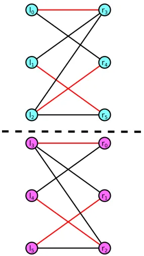
(a)A graph close to bipartite where vertex 2 dominates ver-tex 1
(b) The LR-graph associated with the
bipartite graph in 4.4a. The red edges correspond to the maximum matching
computed by the LPreduction.
close to bipartite, H1 and H2 will be connected but isomorphic to G. In this case, two scenarios
are possible.
The first scenario has the initial extreme optimal solution close to the one when the graph is bipartite. This scenario is illustrated in Figure 4.3. The base graph is simply the graph found
in Figure 4.2a with an edge connecting two vertices in one of the partitions. Applying the LP reduction to the graph in Figure 4.3a produces the LR-graph and corresponding maximum matching
in Figure 4.3b. In this example, the maximum matching partitions the LR-graph into the same
subgraphs as those in Figure 4.2. After computing the extreme optimal solution, all vertices are reduced.
Unless there are vertices with degree 1, there are no dominance relationships in a bipartite graph. It is possible that adding edges to a bipartite graph will introduce dominance relationships. For
example, consider the situation in Figure 4.4. This graph is similar to the graph found in Figure 4.3
except there is an edge between vertices 1 and 2 instead of vertices 0 and 1. In this case, 2 dominates 1 and both the dominance reduction andLPreduction reduce the graph. For dominance, after 2 is reduced, the degree of vertex 4 becomes 1. As a result, the final cover produced by the dominance
reduction is {0,1,2}. For the LP reduction, the resulting LR-graph is partitioned in a manner similar to Figure 4.2. The resulting cover is also{0,1,2}. Regardless, the LPreduction is at least as effective as dominance reduction in this scenario.
Thesecond scenariois when the initial extreme optimal solution contains many non-integer values. Since the graph is close to being bipartite, it is likely that the graph becomes bipartite after
branching and/or other reductions break the problematic odd cycles. Here, theLPreduction is not effective initially, but becomes effective later on.
In the first scenario, theLPreduction reduces at least as many vertices as the dominance reduction; in the second scenario, although the LP reduction is not initially effective, after branching/other reductions are applied, the graph will either become bipartite or match the criteria for first scenario. This leads to our first hypothesis:
Hypothesis 1. TheLPreduction is most effective when applied to graphs that have a small number
of edge disjoint odd cycles.
4.1.1.1 Proximity to Bipartite
In order to explore the validity of our hypothesis, we need a measure that estimates the number of edge disjoint odd cycles. There are many computational problems that can be used to determine how
close a graph is to being bipartite. We focus on the decision problem of given a graph G= (V, E)
and an integer k, does there exist E0 ⊂E with |E0| ≤ k such that G0 = (V, E−E0) is bipartite. This is theBipartite Subgraph Problemand isNP-Complete[GJ79].
We can use a DFS traversal of a graph to get an upper bound by examining back edges. If we
is dependent on the order in which DFS processes vertices, we use the average value over 30
permutations of the ratio between the number of odd cycle vertices counted by DFS and the total number of edges as a proxy measure (denoted as theoc value) to estimate the distance a graph is from being bipartite. Anoc value of 0 means the graph is bipartite.
4.1.2 Degree Distribution
In this section, we examine how the degree distribution of a graph can predict the performance
of reductions. Using information about the vertex degrees to improve the performance of BR
al-gorithms for Minimum Vertex Cover is not a new idea: Xiao and Nagamochi [XN17] present a fast BR algorithm for Minimum Vertex Cover that utilizes the maximum degree of a graph. They accomplish this by first branching on graphs until the maximum degree is less than or equal
to 8; then they apply fast algorithms designed for maximum degree 6, 7, and 8 (which all use more sophisticated reduction rules such as the alternative andk-independent set reductions).
Instead of focusing on the maximum degree as do Xiao and Nagamochi, we focus on the degree
distribution. We begin by stating our next hypothesis:
Hypothesis 2. The degree-one+dominance reductions are most effective when applied to graphs that have degree distributions with high variance.
The intuition behind our claim is a negative one: regular graphs can be difficult to reduce using
the degree-one, dominance, and LP reductions.
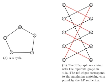
Consider Figures 4.5 and 4.6 which show an example of a 2-regular (an odd length cycle) and a 3-regular graph, respectively. In both cases, no vertex dominates any other vertex. For the 5-cycle in
Figure 4.5, the LR-graph has only one connected component and is notnormalized. As a result, the extreme minimum s-t cut, computed from Algorithm 3 does not contain any left or right vertices so the resulting extreme solution contains no integer values.2 Therefore, theLPreduction does not reduce a vertex. The same is true for the 3-regular graph in Figure 4.6.
4.1.2.1 Degree Variance (dv)
The coefficient of variation of a distribution is defined as the ratio of the standard deviation to the mean. Informally, the coefficient of variation of the degree distribution provides a measure of
how close a graph is to being regular: low coefficient of variation means a graph is close to regular;
high coefficient of variation means the graph has a wide degree distribution, as is the case with, for example, power-law graphs.
2
(a)A 5 cycle
(b) The LR-graph associated
with the bipartite graph in 4.5a. The red edges correspond to the maximum matching
com-puted by theLP reduction.
Figure 4.5 An example of how theLPreduction does not reduce any vertex in a regular graph.
(a)A 3-regular graph
(b) The LR-graph associated
with the bipartite graph in 4.6a. The red edges correspond to the maximum matching
com-puted by theLP reduction.
4.1.3 Edge Density
It is well-known that sparse instances or sparse sub-instances are often more difficult for branch-and-reduce algorithms to solve than denser instances. Many of the recent improvements to the
theoretical runtime complexity of BR algorithms have come from reductions designed for sparse instances [Bou12] [XN17].
In our discussions, we useedge density,m/n, instead ofm/C(n,2), as our density measure. For the degree-one+dominance reductions, edge density can play a big role in how effective the reductions are. On one extreme, any tree is easily reduced by the degree-one reduction. On the other extreme, in
a clique, each vertex dominates every other vertex; as a result, the dominance reduction completely
reduces the graph. Graphs that are close to either extreme might also be easily reduced by the degree-one+dominance reductions. Since very few of the instances used in our experiments have
edge densities close to the maximum, we focused on the relation between the degree-one+dominance
reductions and instances with low edge density.
This leads to our last hypothesis.