INVESTIGATION
A Decision Rule for Quantitative Trait Locus
Detection Under the Extended Bayesian
LASSO Model
Crispin M. Mutshinda*,1and Mikko J. Sillanpää*,†,‡,2 *Department of Mathematics and Statistics and‡Department of Agricultural Sciences, University of Helsinki, FIN-00014 Helsinki, Finland, and†Department of Mathematical Sciences, Department of Biology and Biocenter Oulu, University of Oulu, FIN-90014 Oulu, Finland
ABSTRACTBayesian shrinkage analysis is arguably the state-of-the-art technique for large-scale multiple quantitative trait locus (QTL) mapping. However, when the shrinkage model does not involve indicator variables for marker inclusion, QTL detection remains heavily dependent on significance thresholds derived from phenotype permutation under the null hypothesis of no phenotype-to-genotype association. This approach is computationally intensive and more importantly, the hypothetical data generation at the heart of the permutation-based method violates the Bayesian philosophy. Here we propose a fully Bayesian decision rule for QTL detection under the recently introduced extended Bayesian LASSO for QTL mapping. Our new decision rule is free of any hypothetical data generation and relies on the well-established Bayes factors for evaluating the evidence for QTL presence at any locus. Simulation results demonstrate the remarkable performance of our decision rule. An application to real-world data is considered as well.
W
IDELY recognized to be effective for genomic predic-tion, Bayesian regularization or shrinkage methods are also arguably the state-of-the-art approach to genome-wide multiple quantitative trait locus (QTL) mapping (e.g., Che and Xu 2010). In both the maximum-likelihood (ML) and Bayesian approaches, QTL can be informally identified as locations corresponding to bumps in the plot of the esti-mated genetic effects against marker genomic positions.In Bayesian shrinkage models involving marker inclusion indicators, Bayes factors (BFs) (Kass and Raftery 1995) pro-vide a convenient tool for QTL detection (e.g., Yi et al.
2007). Sillanpää et al. (2012) pointed out that including indicators as an additional source of shrinkage may induce a downward bias on the resulting BFs.
When the Bayesian shrinkage model does not involve marker inclusion indicators, these can still be indirectly
generated with regard to a user-specific effect-size threshold, following Hoti and Sillanpää (2006). However, the subse-quent BFs may heavily depend on the prespecified effect-size cutoff value. Knürret al.(2011) proposed a Bayesian shrink-age model where the marker inclusion indicators are indirectly generated based ona priorifixed and biologically meaningful hyperparameters, allowing the use of BFs to evaluate the strength of evidence in the data in support of QTL presence at any locus.
A QTL significance threshold can alternatively be derived from Wald test statistic (Yang and Xu 2007). This may, how-ever, be unrealistic in the presence of highly correlated markers, due to overly inflated standard errors of the esti-mated genetic effects as a consequence of multicollinearity. Moreover, under the Bayesian shrinkage approach, the pos-terior densities of QTL effects are typically bimodal with a spike at the prior mode (zero) and a second mode around the actual QTL effect (see, e.g., Figure 2 in Che and Xu 2010). This makes equal-tail credibility intervals (Li et al.
2011) impractical for detecting QTL since intervals will of-ten include zero.
In general, rigorous decision making with regard to true and false signals remains an open problem within high-dimensional Bayesian shrinkage analysis (Heaton and Scott 2010). Nevertheless, the phenotype permutation-based (or
Copyright © 2012 by the Genetics Society of America doi: 10.1534/genetics.111.130278
Manuscript received June 21, 2012; accepted for publication August 29, 2012 Supporting information is available online athttp://www.genetics.org/content/early/ 2012/09/14/genetics.111.130278/suppl/DC1.
1Present address: Department of Mathematics and Computer Science, Mount
Allison University, 67 York St., Sackville, NB, E4L 1E6, Canada.
2Corresponding author: Departments of Mathematical Sciences and Biology, PO Box
3000, University of Oulu, FIN-90014 Oulu, Finland. E-mail: [email protected].fi
randomization) method of Churchill and Doerge (1994) is widely used for QTL discovery under both the ML-based (e.g., Churchill and Doerge 1994; Doerge and Churchill 1995) and the Bayesian (e.g., Xu 2003; Mutshinda and Sillanpää 2010) frameworks. The permutation-based method involves the following three stages:
1. Based on the genotypic data at hand, generate a large number of hypothetical phenotypic data under the null hypothesis of no phenotype-to-genotype association by pairing one individual’s genotype with another’s pheno-type to generate data with the observed linkage disequi-librium and no phenotype-to-genotype association. 2. Fit the model to each permuted data set and monitor the
value of a suitable test statistic (e.g., the largest absolute effect size). This yields an empirical distribution of the test statistic under the null hypothesis.
3. Select a specific percentile of this empirical distribution [e.g., the 100·ð12aÞpercentile for a suitable 0,a,1] as the effect-size significance threshold above which to declare QTL.
The permutation-based method is computationally in-tensive. This is more so when the modelfitting is carried out with a Bayesian approach through Markov chain Monte Carlo (MCMC) (Gilks et al.1996) simulation. More impor-tantly, from a Bayesian perspective, the posterior distribu-tion embodies the data-updated state of knowledge about the model parameters and is therefore the sole basis for all inferences, including prediction and hypothesis testing. Bayesian conclusions arise in the form of probabilistic state-ments about unobserved quantities including model param-eters and yet unobserved data (prediction), conditionally on the data actually observed (Gelmanet al. 2003). Thus, the hypothetical data generation under the null hypothesis at the heart of the permutation-based method is inconsistent with the Bayesian philosophy.
In an attempt to mitigate the heavy computational load characterizing the randomization approach in MCMC-based Bayesian shrinkage analysis of QTL, Che and Xu (2010) pro-posed a within-MCMC phenotype permutation approach intended to reduce the computational time burden, but still rooted in the hypothetical data generation at issue with the Bayesian thinking. The authors were the first to recognize the lack of theory behind their method.
Hypothesis testing methods for variable selection that stand firm on the Bayesian philosophy are missing within Bayesian shrinkage analysis of high-dimensional regression models. This article attempts to bridge this gap by proposing a fully Bayesian decision rule for QTL detection under the extended Bayesian LASSO (EBL) model introduced by Mutshinda and Sillanpää (2010).
Methods
Before proceeding to describe our new QTL detection rule, a brief review of the EBL is worthwhile.
The EBL in a nutshell
The EBL (Mutshinda and Sillanpää 2010) extends the hier-archical prior specification of the regression coefficients in the Bayesian LASSO (BL) (Park and Casella 2008; Yi and Xu 2008) with an additional level implementing the separation between the overall model sparsity and the degree of shrink-age specific to individual regression parameters (the marker effects). In simulation studies (Mutshinda and Sillanpää 2010; Fanget al.2012; Kärkkäinen and Sillanpää 2012; Li and Sillanpää 2012), the EBL has proved to be among the best LASSO-type shrinkage methods in terms of estimation and prediction accuracy. Throughout, we consider the fol-lowing multiple linear regression model for QTL mapping,
yi¼b0þ Xp
j¼1
xijbjþei ði¼1;. . .;n; j¼1;. . .;pÞ; (1)
where yi is the phenotypic trait value of theith individual (i¼1;. . .;n), b0 is the common intercept, and xij is the genotype value of individual i at locus j. Here, attention is restricted to experimental crosses derived from inbred lines, more specifically on backcross (BC) or double-haploid (DH) progeny with only one of two possible genotypes at any locus, andxij is coded as 0 for one genotype and 1 for the other.bj is the genetic effect of marker jðj¼1;. . .;pÞ, and ei ði¼1;. . .;nÞ are mutually independent errors assumed to follow a zero-mean Gaussian distribution with common vari-ance s2
0. The EBL is based on the following hierarchical prior specification:yijX; b0;b1;. . .;bpNðb0þ
Pp
j¼1xijbj;s20Þ, for
i¼1;. . .;n independently; and bjjs2j Nð0;s 2 jÞ and s2j jljExpðl
2
j=2Þ independently for j¼1;. . .;p. Each lo-cus-specific regularization parameterlj$0 is further modeled aslj¼dhj, where the quantitiesd$0 andhj.0 are, respec-tively, intended to control the overall model sparsity level and the degree of shrinkage specific tobj, with a largerhjimplying more shrinkage onbj.
Marginally, eachbjhasa prioria zero-mean Laplacian or double-exponential (DE) distribution with variance 2=l2j, according the following representation of the DE distribution as a scaled mixture of normals with exponentially distributed mixing variances: DE ðxj0;l=2Þ ¼ ðl=2Þexp ð2l jxjÞ ¼
RN 0 ð1=
ffiffiffiffiffiffiffiffi 2ps
p
Þexp ð2x2=2sÞðl2=
2Þexp ð2l2s=2Þd s(Park and Casella 2008).
The model specification is completed with prior assump-tions on the parametersb0ands20and the hyperparameters dandhjðj¼1;. . .;pÞ. Our new QTL detection rule operates at the hyperparameter level and more specifically on the idiosyncratic hyperparametershj.
The novel QTL detection rule
Bayesian LASSO arises as a particular case of the EBL when allhjare set to 1, implying thatlj¼l¼dfor 1#j#p. The tenet of our new QTL detection rule is that genuine QTL effects should undergo less shrinkage than implied by the overall model sparsity level determined byd. In other words,
hj should be consistently less than 1 for genuine QTL and vice versa. Biologically, we take the effects of non-QTL loci as reference for comparison, understanding that the effects of actual QTL should not be shrunken beyond the overall model sparsity level.
Our new QTL detection rule is based on the posterior of the locus-specific shrinkage hyperparameters, hj, without involving any hypothetical data generation. Basically, the method boils down to testing the hypothesis Hj1:hj,1 of QTL presence at locusjðj¼1;. . .;pÞ, against the alternative hypothesis Hj2:hj$1 of having no QTL at locus jfor each 1#j#p.
In the Bayesian paradigm, the specification of priors about the model parameters and the hypotheses being tested is a critical stage whereby subjective probability enters the inference. Prior odds can be used to add context to the analysis. For example, model sparsity can be enforced by assigning low prior odds for QTL presence at any locus,i.e., setting PrðHj1Þ ¼Prðhj,1Þ to be small relative to PrðHj2Þ ¼12 PrðH
j
1Þ. As we discuss below, the uniform prior hj Uniðu;wÞ, u,1,w provides much flexibility in cali-brating the prior assumption about Pr ðhj,1Þ and, conse-quently, the prior odds for Hj1,ðj¼1;. . .;pÞ.
More specifically, if we assume a priori that hjUniðu;wÞ, u,1,w independently for j¼1;. . .;p, then the prior probability, PrðH1Þ ¼Pr ðhj,1Þ, of QTL pres-ence at locusjis nothing butð12uÞ=ðw2uÞ. This prior can be duly adjusted through a judicious choice of uandw. In the sequel, we assume, without loss of generality, thatu¼0 so that the prior probability of QTL presence at locus j is simply Pr ðhj,1Þ ¼1=w, the corresponding odds being 1=ðw21Þ.
The essence of a Bayesian analysis is to update prior beliefs about model parameters and hypotheses in light of the observed data. Posterior odds reflect the analyst’s state of knowledge about the relative strengths of two competing and mutually exclusive hypotheses after taking the data in-formation into account. They are therefore well suited to hy-pothesis testing and decision making with regard to QTL presence at different loci. However, Bayes factors provide a better alternative to posterior odds as they free the analyst from reporting prior odds (e.g., Schervish 1995, p. 221) and allow the strength of evidence provided by the data in favor of a hypothesis to be evaluated on the widely used Jeffreys (1961) empirical scale described below.
Let Hj1 and H j
2 denote the hypotheses “QTL present at locus j” and “no QTL at locus j,” corresponding to hj,1 andhj$1, respectively. The Bayes factor
BFj1;2¼Prðhj,1jDataÞ=ð12Prðhj,1jDataÞÞ Prðhj,1Þ=ð12Prðhj,1ÞÞ
(2)
quantifies the evidence provided by the data in favor of Hj1 as opposed to Hj2 (e.g., Berger 1985, p. 146), with BFj1;2.1 implying more evidence in support of Hj1than assumeda pri-ori, and vice versa. Jeffreys (1961) provided the following
scale for evaluating the strength of evidence for Hj1 vs.H j 2: BFj1;2,1, negative support for H
j
1 (i.e., support for H j 2); 1#BFj1;2,3, a support for H
j
1that is barely worth mention-ing; 3#BFj1;2,10, substantial support for H
j 1; 10# BFj1;2,100, strong support for H
j
1; and BF j
1;2.100, decisive support for Hj1.
Our new decision rule for QTL detection is based on the Bayes factor BFj1;2defined in (2) and, as a rule of thumb, we use 3 as the cutoff value of BFj1;2above which to declare QTL presence at locus j. The choice of this somewhat stringent cutoff value is motivated by the need to optimize the power of detecting QTL by reducing the false discovery rate.
A critical quantity for the computation of the Bayes factor BFj1;2 is the posterior probability Pr ðhj,1DataÞ. A Monte Carlo-based estimate of this probability under MCMC sam-pling is given by Pr ðhj,1jDataÞ ð1=NmÞ
PNm i¼1Iðhð
iÞ j ,1Þ, whereIð:Þdenotes the indicator function,Nmis the number of post-burn-in MCMC samples, and hðiÞj is the ith MCMC sample for hj. This probability is easily evaluated in Win-BUGS/OpenBUGS through the logical function step(.) that takes the value 1 when its argument is larger than zero and the value zero otherwise. For more details on this, see sup-porting information,File S1.
We next report on two simulation studies designed to investigate the performance of our new QTL detection rule under different scenarios. We subsequently utilize our de-cision rule to reanalyze the genetic basis of time to heading in barley (Hordeum vulgareL.), using real-world data from the North American Barley Genome Mapping project (Tinker
et al.1996).
Report on simulation studies
To evaluate the performance of our new decision rule for QTL detection, we carried out two simulation studies, hereafter simulation study 1 and simulation study 2. Simu-lation study 1 involved two replicated analyses based, respectively, on the moderately dense barley marker data and on a computer-simulated dense marker data set. Simu-lation study 2 was based on a very dense and particularly challenging marker data set generated through computer simulation.
Simulation study 1:This simulation study is based on the following two marker data sets differing in both the marker density and then-to-pratio:
1. The real-world marker data set from the North American Barley Genome Mapping project (Tinker et al. 1996), which involves 145 DH lines and 127 biallelic markers covering seven chromosomes, the distance between con-secutive markers being 10.5 cM: We refer to Tinkeret al.
(1996) for more details on this data set. The few missing genotypes were imputed with random draws from Ber-noulli(0.5) before the analysis. A more appropriate ap-proach to missing genotype imputation would be to utilize their genotype probabilities given the genotypes
of flanking markers with regard to a genetic map (see Jiang and Zeng 1997).
2. A dense marker data set simulated through the WinQTL Cartographer 2.5 program (Wanget al.2006), compris-ing 50 backcross progeny and 102 markers (approxi-mately twice as many markers as individuals) spanning three chromosomes with 34 evenly spaced markers each and just 3 cM between consecutive markers.
In both cases, the phenotypic trait values were simulated assuming sparse underlying biology with only four QTL at loci 4, 25, 50, and 65, with respective effects 2.5,22.5, 4, and24. In the data simulation process, the intercept was set to zero without loss of generality. The residual variance,s2
0, was set to 2 and 1 under the barley marker data and the simulated dense marker data, respectively, yielding an ap-proximate heritability of 0.80 in both cases. Our analyses are based on data with high heritabilities and small sample sizes. Sillanpää and Hoti (2007) pointed out that, with regard to power analysis, similar results arise under small heritabilities and large samples.
One hundred phenotype replicates were simulated under each marker data set. The R codes for generating the replicated phenotypic data are provided in File S1, along with the simulated dense marker data and a realization of the simulated phenotypes under the parameter setting de-scribed above. A typical vector of simulated phenotypes un-der the barley marker data is provided as well.
The model specification was completed with the following (essentially noninformative) prior specification:b0Nð0;100Þ; and s2
0 Inv-Gamma ð0:01;0:01Þ, dUnið0;100Þ, and hj Unið0;wÞ for j¼1;. . .;p independently. Finally, w
was set to 10, yielding a prior probability Prðhj,1Þ ¼0:1 of QTL presence at any locusjð1#j#pÞ.
We used MCMC simulation, through the Bayesian free-ware OpenBUGS (Thomaset al.2006), to sample from the joint posterior of the model parameters. The BUGS code is available inFile S1. All computations were carried out on an AMD Turion X2 Dual, with a 64-bit operating system and 4 GB of RAM. We initially ran three Markov chains for 100,000 iterations to assess, through visual inspection of traceplots, the time to convergence and the quality of the mixing of the chains. The Markov chains reached apparently their target distributions after500 and 2000 iterations un-der the barley data and the simulated dense marker data set, respectively. The 100,000 iterations of three Markov chains took7 hr under the barley data and 2 hr under the simu-lated dense marker data set.
We thenfitted the model to the 100 replicated data sets, running a single Markov chain for 7000 iterations after a burn-in period of 3000 iterations and thinning the re-mainder to each 10th sample. The model fitting to each replicated data set took 770 sec under the barley marker data and 420 sec under the simulated dense marker data set. Figure 1 shows the Bayes factors for QTL presence at each marker locus on a natural logarithmic scale, averaged
over the 100 replicated data sets plotted against the marker genomic positions for simulations based on the barley marker data (Figure 1A) and the simulated dense marker data set (Figure 1B). In Figure 1, A and B, the threshold, logð3Þ 1:1, above which QTL are declared is indicated by a horizontal shaded dashed line.
From the results plotted in Figure 1, the four“true”QTL are clearly singled out with BFs far larger than the cutoff value logð3Þ 1:1, in contrast to the non-QTL candidate loci. The four QTL were also the only loci with BFs exceed-ing the detection threshold under the barley marker data set, implying a false discovery rate of 0%. The BFs for QTL presence at non-QTL loci were consistently ,1 and did not even approach the selection threshold in the few cases where they happened to exceed 1. In analyses based on the simulated dense marker data set, some loci close to the actual QTL locations could occasionally have BFs.1 due to linkage disequilibrium, but these should not be consid-ered as false positives.
We also evaluated the performance of the permutation-based method for QTL detection under the EBL with the parameter setting described above, using 100 phenotype permutations. For each permuted data set, we ran 15,000 iterations of a single Markov chain and discarded the first 4000 iterations as burn-in, thinning the remainder to each 10th sample.
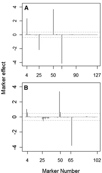
Figure 2 shows the posterior mean genetic effects aver-aged over the 100 replicated data sets, plotted against the
Figure 1 (A and B) Natural logarithms of the Bayes factors for QTL pres-ence at each marker plotted against the marker number, averaged over 100 replicated data sets under the barley marker data (A) and the simu-lated dense marker data (B). The horizontal shaded dashed line indicates the log(BF) threshold, logð3Þ 1:1, above which QTL are declared.
marker numbers for analyses based on the barley marker data (Figure 2A) and for those based on the simulated dense marker data set (Figure 2B). The horizontal shaded dashed lines therein represent the permutation-based effect size thresholds for declaring QTL.
It seems that QTL 25 could be missed under a number of data replicates. From Figures 1B and 2B, one can realize that the correlation among markers is high in the vicinity of QTL 25. On the other hand, we know that the effect of QTL 25 was simulated to be relatively small. This suggests that the permutation-based method may be ineffective at detecting small-effect size QTL in the presence of strongly correlated markers, in contrast to the method proposed here (Figure 1). Onea priorifor this may be that in MCMC-based Bayes-ian replicated data analysis, permutation thresholds are of-ten, as is also the case here, based on a single realization so that its behavior may heavily depend on the particular data realization under consideration. Moreover, Churchill and Doerge (1994) emphasized that a large number of pheno-type permutations are required to produce a more accurate estimate of the critical value. With the MCMC-based Bayes-ian approach, one should also ensure that the MCMCs are run long enough under each phenotype permutation and not rely on a small number of permutations. With the ap-proach proposed here, the MCMCs are run only once, with no extra computational cost required for variable selection
that is a by-product of the model-fitting effort, rather than the result of a post–model-fitting exercise as is the case for the permutation-based counterpart.
Simulation study 2: In simulation study 1 we simulated dense markers with 3-cM intervals, mimicking a realistic inbred line cross situation where recombination occurs rarely between adjacent markers. Although it is unneces-sary for researchers to screen their BC or DH populations at each centimorgan, we simulate a marker map with 1 cM distance between consecutive markers to investigate how well our method would perform when faced with such a situation where the dependency between markers is very high. Mutshinda and Sillanpää (2012) simulated marker maps of inbred line-cross data with 1-cM intervals to evalu-ate the performance of their procedures.
The marker data set was simulated through the WinQTL Cartographer 2.5 program (Wanget al.2006) and involved 50 BC progeny and 200 markers (i.e., four times as many markers as individuals), with just 1 cM between consecutive markers.
The phenotypic trait values were simulated assuming seven QTL, namely at loci 6, 12, 71, 75, 120, 185, and 192, with respective effects22.5,21.5, 3,23, 4,21.5, and25. The residual variance was set to 8 in the data simulation process, yielding an approximate heritability of 0.80.
Note that in extremely oversaturated regression models, the intercept mayfluctuate greatly and capture most of the signal since no shrinkage is imposed on it, which may erode the model’s ability to discriminate the effects of different predictors (loci). This is more so when no prior covariance structure is assumed for the regression coefficients (genetic effects) as is the case here (cf. Mutshinda and Sillanpää 2012). It would be worth checking whether this problem would be less acute under a different genotype codinge.g.,
21 and 1 rather than the 0 and 1 coding used here. Anyway, we found that this problem can be mitigated by centering the response variable (phenotype) before the analysis (i.e., subtracting its mean from individual values) and forcing the intercept to be zero during estimation. We adopted this ap-proach here without rescaling the phenotypic values to unit variance to maintain the estimated genetic effects on the scale of the simulated values so that we can appreciate the extent of the model-induced shrinkage on individual locus effects.
As a word of caution, the prior inclusion probability should not be selected to be too small in extremely oversaturated regression models (i.e., when pn) or when the correla-tion among predictors (markers) is very high, to preserve the good mixing property. A similar problem has been pointed out to occur in spike-and-slab methods (e.g., O’Hara and Sillanpää 2009). Recall that Pr ðhj,1Þ is controlled by the prior setting ofhjor, more specifically in our case, by the value ofw. In analyzing this particularly challenging data set, we set the hyperparameter wto 4, yielding a prior inclusion proba-bility Pr ðhj,1Þ= 0.25 for each marker, which is comparable
Figure 2 (A and B) Posterior mean genetic effects averaged over 100 replicated data sets against the marker numbers for simulations based on the barley marker data (A) and the simulated dense marker data set (B). The horizontal shaded dashed lines represent the effect size thresholds for declaring QTL, based on 100 phenotype permutations.
to prior inclusion probabilities typically used in spike-and-slab variable selection methods.
The simulated marker data set is provided in File S1, along with a typical vector of simulated phenotypic values and the R code for phenotype generation.
In MCMC-based Bayesian shrinkage QTL analysis, when a QTL is correlated with nearby markers, the posterior kernel density plots of its genetic effect typically display a two-component mixture (bimodal) structure. One of the two mixture components is clustered around zero (the prior mode). As more Markov chain iterations are run, a second mode emerges by the actual QTL effect, and the mixture component concentrated around zero becomes increasingly peaked at its mode. It is crucial in such circumstances that MCMC samplers be run much longer to generate enough samples from the emerging mixture components in the posteriors of QTL effects.
We ran 200,000 iterations of two MCMC chains. The chains seemed to reach their target distribution after 7000 iterations. We discarded thefirst 25,000 iterations as burn-in and thinned the remaining MCMC draws to each 25th sample. The 200,000 iterations of two Markov chains took12 hr.
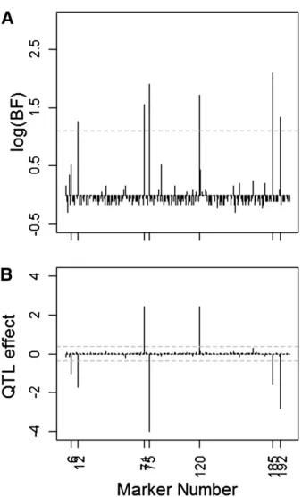
The performance of our method on this challenging data set is illustrated in Figure 3A, where the Bayes factors for
QTL presence at each marker locus are plotted on a natural logarithmic scale against the marker position for a single-phenotype realization. The horizontal shaded dashed line indicates the threshold above which QTL are declared.
To verify the ability of the phenotype permutation-based method to identify QTL in the presence of highly correlated markers, we required 100 phenotype permuted data sets. For each permutated data set, we ran 25,000 iterations of a single Markov chain, discarding thefirst 8000 samples as burn-in and thinning the remainder by a factor of 10. The 25,000 iterations took 2122 sec. Figure 3B shows the pos-terior means of genetic effects with the permutation thresh-old indicated by the overlaid horizontal shaded dashed line. It can be seen from Figure 3A that a few adjacent loci to actual QTL positions were also selected, due to linkage dis-equilibrium. The BFs for QTL presence at actual QTL positions were much larger, making them plainly distinguishable from non-QTL loci through our decision rule (except locus 6). The posterior means of genetic effects for a single phenotype re-alization are shown in Figure 3B, where the horizontal shaded dashed lines therein indicate the effect size thresholds for declaring QTL, based on 100 phenotype permutations.
Real data analysis
We utilized our new decision rule for QTL detection to reanalyze the genetic basis of the time to heading in barley, using real-world data from the North American Genome Mapping project (Tinker et al.1996). As mentioned above, the mapping population comprises 145 doubled haploid lines after 5 individuals with missing phenotype have been omitted. Each progeny was scored at 127 markers covering seven chromosomes. The phenotypic trait of interest is the number of days to heading, averaged over 25 different envi-ronments. The phenotypic trait values were standardized to have mean zero and unit variance, and the few missing genotypes were imputed with random draws from Ber-noulli(0.5) before the analysis.
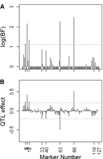
The model fitting to the data was carried out by MCMC simulation through OpenBUGS under the same prior specifi -cation as in simulation study 1. We ran 20,000 iterations of two MCMC chains after a burn-in period of 5000 iterations and applied a thinning factor of 10, which resulted in 4000 draws. Figure 4, A and B, shows, respectively, the BFs for QTL presence and the posterior mean genetic effects at different loci. The horizontal shaded dashed line in Figure 4A repre-sents the log(BF) threshold, logð3Þ 1:1, above which QTL are declared, whereas the ones in Figure 4B represent the permutation-based thresholds above which to declare QTL. These cutoff values are based on 100 phenotype permutations. The results shown in Figure 4 imply that the genetic basis of the time to heading in barley is sparse. Five loci only, namely loci 6, 9, 12, 63, and 86, emerged as actual QTL, with BFs for QTL presence exceeding the cutoff value of 3. All loci with BFs for QTL presence.1 are listed in Table 1, wherein boldface type is used to indicate the BFs exceeding the QTL detection threshold.
Figure 3 (A) Natural logarithms of the Bayes factors for QTL presence at each marker, plotted against the marker number for a single-phenotype realization under the very dense marker data, with the horizontal shaded dashed line indicating the log(BF) threshold, logð3Þ 1:1, above which QTL are declared. (B) Posterior means of genetic effects for a single-phe-notype realization under the very dense marker data. The horizontal shaded dashed lines represent the effect size thresholds for declaring QTL, based on 100 phenotype permutations.
We also performed a randomization test for QTL discov-ery, using the highest posterior inclusion probability, and hence the highest BF, as a test statistic. The posterior marker inclusion probabilities are shown in Figure 5. Therein, the permutation-based cutoff value for QTL selection based on 100 phenotype permutations, 0.15, corresponding to a BF of 1.588 is indicated by the horizontal shaded dashed line. The solid dashed line indicates the QTL inclusion probability 0.25, which corresponds to our rule-of-thumb threshold BF¼3 for QTL selection under the prior inclusion probabil-ity Pr ðhj,1Þ ¼0:10 adopted here.
The randomization approach has led to the selection of some additional loci, namely loci, 3, 5, 33, 40, 47, 78, 119, and 120, which are mostly among the loci with BFs .1 under our decision rule.
Knürret al. (2011) also analyzed the time to heading in barley, using the same data set, and identified 12 markers, 10 of which are among the loci with Bayes factors for inclusion
.1, which are given in Table 1. The BFs for the two other loci, namely locus 44 and locus 55, were,1 in our analysis.
Discussion
In this article, we proposed a fully Bayesian decision rule for QTL detection under the EBL introduced by Mutshinda and Sillanpää (2010). In simulation studies (Mutshinda and
Sillanpää 2010; Fanget al.2012; Kärkkäinen and Sillanpää 2012; Li and Sillanpää 2012), the EBL has proved to be among the top LASSO-type shrinkage methods with regard to QTL detection, owing presumably to its ability to explic-itly distinguish the overall model sparsity from the degree of shrinkage idiosyncratically experienced by the regression coefficients. Since true QTL effects are expected to experi-ence less shrinkage than assumed by the overall model spar-sity level, their individual shrinkage hyperparameters should consistently be,1. Consequently, QTL detection can be based on whether a locus-specific shrinkage hyperparameter is,1. If these hyperparameters are assigned suitable (uniform) priors that can be understood in terms of marker inclusion/ exclusion, QTL detection can rely on their posterior distribu-tions. The posterior inclusion probabilities of different loci, and hence the corresponding Bayes factors, can be used to evaluate the strength of evidence for QTL presence at differ-ent loci with regard to a suitable cutoff value. This is what our QTL detection rule is all about.
Simulation results (Figures 1–3) demonstrated the effec-tiveness of our new detection rule to identify QTL, including in very challenging situations. For example, in simulation study 2, the QTL 71 and 75 simulated to be physically close, but with opposite signs were effectively detected (Figure 3), although this is generally difficult in practice as pointed out by Wanget al.(2005).
It has been noted earlier that under the MCMC estimation context where uniform priors can be easily assumed, EBL shows no need for tuning of hyperparameters (Mutshinda and Sillanpää 2010) while in a maximum a posteriori esti-mation context, tuning of the Gamma hyperparameters is critical (Kärkkäinen and Sillanpää 2012; Li and Sillanpää 2012; Mutshinda and Sillanpää 2012). Accordingly, our results were robust to the values of u and w defining the range of the uniform prior imposed on the hyperparameters hj, j¼1;. . .;p. However, the Bayes factors may in some cases be sensitive to the choice ofuandw, and the suitable
Figure 4 (A) Natural logarithms of the Bayes factors for QTL presence at each marker with regard to the phenotypic trait “number of days to heading,”using the North American Barley data, plotted against marker numbers. The horizontal shaded dashed line indicates the log(BF) thresh-old, logð3Þ 1:1, above which QTL are declared. (B) Posterior means of genetic effects on the time to heading in North American barley. The horizontal shaded dashed lines represent the effect size thresholds for declaring QTL, based on 100 phenotype permutations.
Table 1 List of loci with Bayes factors for QTL presence.1, with boldface type indicating BFs that exceed the QTL detection threshold of 3
Marker ID BF
5 1.58
6 3.16
9 8.64
10 1.34
12 3.86
33 2.40
40 2.25
47 1.59
49 1.34
51 1.11
62 1.34
63 9.75
86 12.00
115 1.34
118 1.58
119 1.58
BF threshold for detecting QTL may be data dependent as pointed out by Knürret al.(2011). A sensitivity analysis is therefore necessary.
In cases where the model is excessively overparameter-ized, or when the level of correlation between markers is extremely high, one may proceed stepwise by firstfiltering the data by discarding all loci with BFs for QTL presence,1 and then refitting the mapping model to the reduced data set. The modelfitting to afiltered data set generally results in improved accuracy of the estimated genetic effects (see,
e.g., Mutshinda and Sillanpää 2011). One may alternatively proceed by placing pseudomarkers in every interval of a pre-specified length (e.g., every 5 cM as in Che and Xu 2010) and base the mapping analysis on these pseudomarkers, with their genotypes inferred (or imputed) using, for exam-ple, the multipoint method (Jiang and Zeng 1997).
In our evaluation, we used the permutation-based method as proposed by Churchill and Doerge (1994). The within-MCMC permutation-based method of Che and Xu (2010) is just a more computationally efficient approach to the origi-nal method of Churchill and Doerge (1994) and should ideally lead to similar results. On the other hand, the method of Che and Xu (2010) builds on the Bayesian shrink-age regression model of Xu (2003) as extended by Ter Braak
et al.(2005), which does not involve the separation feature of the EBL on which our method is based. Hoti and Sillanpää
(2006) pointed out mixing problems and sensitivity to start-ing values with the model of Xu (2003) under highly corre-lated predictors (markers and gene expressions) and small sample size, which is apparently not the case for EBL.
It would be interesting to examine whether the intro-duction of the separation feature in Xu’s (2003) model as extended by Ter Braak et al.(2005) would alleviate these problems and to further investigate how well the QTL de-tection method proposed here would perform under such a model.
Acknowledgments
We thank the Associate Editor and two anonymous referees for constructive comments on the manuscript. This work was supported by research grants from the Academy of Finland and the University of Helsinki’s research funds.
Literature Cited
Berger, J. O., 1985 Statistical Decision Theory and Bayesian Anal-ysis, Ed. 2. Springer-Verlag, New-York.
Che, X., and S. Xu, 2010 Significance test and genome selection in Bayesian shrinkage analysis. Int. J. Plant Genomics 2010: 893206.
Churchill, G. A., and R. W. Doerge, 1994 Empirical threshold values for quantitative trait mapping. Genetics 138: 963–971. Doerge, R. W., and G. A. Churchill, 1995 Permutation tests for
multiple loci affecting a quantitative character. Genetics 142: 285–294.
Fang, M., D. Jiang, D. Li, R. Yang, W. Fu et al., 2012 Improved LASSO priors for shrinkage quantitative trait loci mapping. Theor. Appl. Genet. 124: 1315–1324.
Gelman, A., J. B. Carlin, H. S. Stern, and D. B. Rubin, 2003 Bayes-ian Data Analysis, Ed. 2nd. Chapman and Hall, New York. Gilks, W. R., S. Richardson, and D. J. Spiegelhalter, 1996 Markov
Chain Monte Carlo in Practice, Chapman and Hall, London, UK. Heaton, M., and J. Scott, 2010 Bayesian computation and the linear model, pp. 527–545 in Frontiers of Statistical Decision Making and Bayesian Analysis, chap 14., edited by M. H. Chen, D. K. Dey, P. Muller, D. Sun, and K. Ye. Springer, New York. Hoti, F., and M. J. Sillanpää, 2006 Bayesian mapping of genotype
x expression interactions in quantitative and qualitative traits. Heredity 97: 4–18.
Jeffreys, H., 1961 Theory of Probability, Clarendon Press, Oxford. Jiang, C., and Z.-B. Zeng, 1997 1997 Mapping quantitative trait loci with dominant and missing markers in various crosses from two inbred lines. Genetica 101: 47–58.
Kärkkäinen, H. P., and M. J. Sillanpää, 2012 Robustness of Bayes-ian multilocus association models to cryptic relatedness. Ann. Hum. Genet. (in press).
Kass, R. E., and A. E. Raftery, 1995 Bayesian factors. J. Am. Stat. Assoc. 90: 773–795.
Knürr, T., E. Läärä, and M. J. Sillanpää, 2011 Genetic analysis of complex traits via Bayesian variable selection: the utility of a mixture of uniform priors. Genet. Res. 93: 303–318. Li, J., K. Das, G. Fu, R. Li, and R. Wu, 2011 The Bayesian LASSO for
genome-wide association studies. Bioinformatics 27: 516–523. Li, Z., and M. J. Sillanpää, 2012 Estimation of quantitative trait
locus effects with epistasis by variational Bayes algorithms. Ge-netics 190: 231–249.
Mutshinda, C. M., and M. J. Sillanpää, 2010 Extended Bayesian LASSO for multiple quantitative trait loci mapping and unob-served phenotype prediction. Genetics 186: 1067–1075.
Figure 5 Posterior marker inclusion probabilities for the number of days to heading in barley. The cutoff posterior probability for QTL selection based on 100 phenotype permutations, 0.15, is indicated by the horizon-tal shaded dashed line. This probability corresponds to a BF of 1.588 under the prior inclusion probability Prðhj,1Þ ¼0:10 adopted here.
The horizontal solid dashed line indicates the probability 0.25, which corresponds to our rule-of-thumb Bayes factor 3 for QTL detection under our prior QTL inclusion probability.
Mutshinda, C. M., and M. J. Sillanpää, 2011 Bayesian shrinkage analysis of QTLs under shape-adaptive shrinkage priors, and ac-curate re-estimation of genetic effects. Heredity 107: 405–412. Mutshinda, C. M., and M. J. Sillanpää, 2012 Swift block-updating
EM and pseudo-EM procedures for Bayesian shrinkage analysis of quantitative trait loci. Theor. Appl. Genet. (in press) DOI:10.1007/ s00122–012–1936–1.
O’Hara, R. B., and M. J. Sillanpää, 2009 A review of Bayesian variable selection methods: what, how and which. Bayesian Anal. 4: 85–118.
Park, T., and G. Casella, 2008 The Bayesian Lasso. J. Am. Stat. Assoc. 103: 681–686.
Schervish, M. J., 1995 Theory of Statistics, Springer-Verlag, New-York. Sillanpää, M. J., and F. Hoti, 2007 Mapping quantitative trait loci from a single tail sample of the phenotype distribution including survival data. Genetics 177: 2361–2377.
Sillanpää, M. J., P. Pikkuhookana, S. Abrahamsson, T. Knürr, A. Frieset al., 2012 Simultaneous estimation of multiple quanti-tative trait loci and growth curve parameters through hierarchi-cal Bayesian modeling. Heredity 108: 134–146.
Ter Braak, C., M. Boer, and M. C. A. M. Bink, 2005 Extending Xu’s Bayesian model for estimating polygenic effects using markers of the entire genome. Genetics 170: 1435–1438.
Thomas, A., R. B. O’Hara, U. Ligges, and S. Sturtz, 2006 Making BUGS Open. R News 6: 12–17.
Tinker, N. A., D. E Mather, B. G. Rosnagel, K. J. Kasha, and A. Kleinhofs, 1996 Regions of the genome that affect agro-nomic performance in two-row barley. Crop Sci. 36: 1053– 1062.
Wang, H., Y-M. Zhang, X. Li, G. L. Masinde, and S. Mohanet al., 2005 Bayesian shrinkage estimation of quantitative trait loci parameters. Genetics 170: 465–480.
Wang, S., C. J. Basten, and Z.-B. Zeng, 2006 Windows QTL Car-tographer 2.5. Department of Statistics, North Carolina State University, Raleigh, NC.
Xu, S., 2003 Estimating polygenic effects using markers of the entire genome. Genetics 163: 789–801.
Yang, R., and S. Xu, 2007 Bayesian shrinkage analysis of quanti-tative trait loci for dynamic traits. Genetics 176: 1169–1185. Yi, N., and S. Xu, 2008 Bayesian Lasso for quantitative trait loci
mapping. Genetics 179: 1045–1055.
Yi, N., D. Shriner, S. Banerjee, T. Mehta, D. Pompet al., 2007 An efficient Bayesian model selection approach for interacting QTL models with many effects. Genetics 176: 1865–1877.
Communicating editor: I. Hoeschele
GENETICS
Supporting Information http://www.genetics.org/content/early/2012/09/14/genetics.111.130278/suppl/DC1
A Decision Rule for Quantitative Trait Locus
Detection Under the Extended Bayesian
LASSO Model
Crispin M. Mutshinda and Mikko J. Sillanpää
C. M. Mutshinda and M. J. Sillanpää 2 SI
File S1
Supporting Information
OpenBUGS code
#############################################################################
model{
for(i in 1:n){
y[i]~dnorm(mu[i],prec)
mu[i]<-alpha + inprod(x[i,], beta[])
}
for (j in 1: p){
beta[j]~dnorm(0,tau[j])
tau[j]<-1/var[j]
var[j]~dexp(w[j])
w[j]<-pow(lambda[j],2)/2
lambda[j]<-lbda*eta[j]
eta[j]~dunif(0,10)
s[j]<-step(1-eta[j])
}
sd~dunif(0,10)
sigma2<-sd*sd
prec<-1/sigma2
lbda~dunif(0, 100)
alpha~dnorm(0, 0.01)
}
#############################################################################
Let
s
j=
I
(
η
j<
1
|
Data
)
. An estimate of the posterior inclusion probability for marker
j
under
our decision rule,
Pr
(
η
j<
1
|
Data
)
, is given by
E
[
s
j]
. This quantity is easily obtained in
WinBUGS/OpenBUGS by simply including
s
j<
−
step
(
1
−
η
j)
to the BUGS code (see above)
C. M. Mutshinda and M. J. Sillanpää 3 SI
Simulated phenotype under the barley marker data
#############################################################################
y=c(-4.4755208193005, -1.06940050265062, 4.87237409484387, 6.79066589577583, 0.483975888797228, -5.27990860440515, -4.89108300540457, 1.14272375642966, 2.57637259192694, -1.430766910525, -3.36723333318214, -0.0153388104315005, -0.162835954798986, 2.83536950265494, 2.6128731055629, -0.437703164732762, 3.02644491587748, -1.62665839105249, -0.288058061848415, -0.681375282254409, -4.69871291863845, 3.69669520834022, 0.906874193688093, 1.15981138051307, -1.54389335987092, -1.25535542695451, -0.849396378491686, -1.78819175635762, 2.64744935983643, -5.77469768422738, 2.35723678395617, -5.46052168440255, -4.03469801481428, 0.795986476026644, -1.18605247885068, -3.73280163391129, 2.37519127477548, -0.971308345369541, 2.43266449022648, -2.48515623301456, 7.07367270018502, 1.82062034924873, -1.61639290386188, -4.36750202303927, 3.7290900538335, -6.30556972838993, -1.81774078500601, 4.94641680724368, 3.18085539065336, 6.3913277949111, -1.45466000430324, 4.65575968233052, -4.89698903550715, -8.15880170481863, -6.32560127040587, 2.85134017569016, 2.26080250149806, -0.135289584361961, -5.49984104125293, -3.27257409305169, -4.24677113805059, 2.56838460242192, -0.536691775599305, 2.95851287926479, -2.93405976123824, -2.21335524102037, 3.25862273290392, -0.49348527447816, 3.67905126256138, -1.06504912727618, 2.41816372295265, -4.14975110190246, 4.3618727847274, -4.57674871541325, 1.32753134209142, 3.82267920413127, -0.116856493147793, 1.00515605707328, 0.666513714753329, 2.47718530744082, -7.67453279464087, 1.35254351043531, 1.59313707897193, 3.94325407440631, -2.26772691136038, 0.269231484706854, -2.81453197313347, -1.38967523198622, -0.612498433319447, -0.486003177994731, 3.23544928077243, -2.73158961885822, 5.19029589787354, -2.39942513682678, -3.50741739861117, 1.41673062175495, 1.40453780368736, 0.0110630170077651, 2.49596355738983, -1.08068313627991, -2.41127247650071, 1.26790264600107, -0.230870326978664, -3.83762601435563, 1.12656514737589, 3.02184635241111, 6.44717055947001, 3.49789967964755, 0.170485059021785, -1.6103501322836, 3.55402004813255, 0.881780571761232, -0.543241973590207, -2.83608015014054, 1.29880753789797, -3.32509109056517, 4.69788344322983, 1.69980132867673, -2.82572273019081, -5.31783596748496, 3.19532627869322, -0.52953776481683, 0.903695616251948, -2.39462243134407, 6.21492337318839, -4.53315619632256, 1.80135491648431, -3.2853584208569, 2.59385006869002, -1.78062292618856, 4.56845369093539, -3.97250017951868, 3.01750279913739, -0.143297006284117, 5.39388349999236, -7.10197468148697, -0.456845908936002, 2.05606662864364, -5.09489082996234, 0.266387459645182, -3.88268874376827, -2.06041622957327, 5.20842956406487, -3.33923277802675, -3.49974698770439)
C. M. Mutshinda and M. J. Sillanpää 4 SI
The simulated dense marker dataset involving 50 individuals and 102 markers
#############################################################################
list( n=50, p=102,y =c(3.86282652415903, 6.6195315019137, -0.531823277667612, 6.326137199428, 5.45036591094395, 3.73404908364244, 0.415379270644612, -3.96755745114551, 1.72333907516979, -4.82756165290557, 0.28649632904341, 1.87331083592723, 2.68565841349693, 5.27512369096443, -2.56610434151942, 1.21337335772993, -6.87005800701743, -3.41046495685588, -4.13661757877691, 5.28229720709657, 0.456718544981508, 4.24496283492176, 0.505195053413676, 4.03719935886078, 0.0215644071086891, 2.41800428535642, 1.28371109227575, -4.32295548437459, 4.08726902111166, 3.89024820139512, -1.86208837286753, 0.446822728375693, 3.20311180157224, 3.72539335391788, 2.68881303116069, -2.68759877527431, 2.35071508366683, 0.377837787174872, 0.57079898362225, 0.762118949924526, -4.66697048848522, -2.33749981949889, 1.51899178039357, 1.49439108267275, 1.24964265649317, 1.46251035441612, 0.499065250024612, -2.92735081507619, 4.29899062537944, -1.44987622809231),
x=structure(.Data=c(0, 0, 0, 0, 0, 0, 0, 0, 0, 0, 0, 0, 0, 0, 0, 0, 0, 0, 0, 0, 0, 0, 0, 0, 0, 0, 0, 0, 0, 0, 0, 0, 0, 0, 1, 1, 1, 1,
C. M. Mutshinda and M. J. Sillanpää 5 SI
C. M. Mutshinda and M. J. Sillanpää 6 SI
C. M. Mutshinda and M. J. Sillanpää 7 SI
C. M. Mutshinda and M. J. Sillanpää 8 SI
0, 0, 0, 0, 0, 0, 0, 0, 0, 0, 0, 0, 0, 0, 0, 0, 0, 0, 1, 1, 1, 1, 1, 1, 1, 1, 1, 1, 1, 1, 1, 1, 1, 1, 1, 1, 1, 1, 1, 1, 1, 1, 1, 1, 1, 1, 1, 1, 1, 1, 1, 1, 0, 0, 0, 0, 0, 0, 0, 0, 1, 1, 1, 1, 1, 1, 1, 1, 1, 1, 1, 1, 1, 1, 1, 1, 1, 1, 1, 1, 1, 1, 0, 0, 0, 0, 0, 0, 0, 0, 0, 0, 0, 0, 0, 0, 0, 0, 0, 0, 0, 0, 0, 0, 0, 0, 0, 0, 0, 0, 0, 0, 1, 1, 1, 1, 1, 1, 1, 1, 1, 1, 1, 1, 1, 1, 1, 1, 1, 1, 1, 1, 1, 1, 1, 1, 1, 1, 1, 1, 1, 1, 1, 1, 1, 1, 1, 1, 1, 1, 1, 1, 1, 1, 1, 1, 0, 0, 0, 0, 0, 0, 0, 0, 0, 0, 0, 0, 1, 1, 1, 1, 1, 1, 1, 1, 1, 1, 1, 1, 1, 1, 1, 1, 1, 1, 1, 1, 1, 1, 1, 1, 1, 1, 1, 1, 0, 0, 0, 0, 0, 0, 0, 0, 0, 0, 0, 0, 0, 0, 0, 0, 0, 0, 0, 0, 0, 0, 1, 1, 1, 1, 1, 1, 1, 0, 0, 0, 0, 0, 0, 0, 0, 0, 0, 0, 0, 0, 0, 0, 0, 0, 0, 0, 0, 0, 0, 0, 0, 0, 0, 0, 1, 1, 1, 1, 1, 1, 1, 1, 1, 1, 1, 1, 1, 1, 1, 1, 1, 1, 1, 1, 1, 1, 0, 0, 0, 0, 0, 0, 0, 0, 0, 0, 0, 0, 1, 1, 1, 1, 1, 1, 1, 1, 1, 1, 1, 1, 1, 1, 1, 1, 1, 1, 1, 1, 1, 1, 1, 1, 1, 1, 1, 1, 1, 1, 1, 1, 1, 1, 0, 0, 0, 0, 1, 1, 1, 1, 1, 1, 1, 1, 1, 1, 1, 1, 1, 1, 1, 1, 1, 1, 1, 1, 1, 1, 1, 1, 1, 1, 1, 1, 1, 1, 1, 1, 1, 1, 1, 1, 1, 1, 1, 1, 1, 1, 1, 1, 1, 1, 1, 1, 1, 1, 1, 1, 1, 1, 1, 1, 1, 1, 1, 1, 1, 1, 1, 1, 0, 1, 1, 1, 1, 1, 1, 0, 1, 1, 1, 1, 1, 1, 1, 1, 1, 1, 1, 1, 1, 1, 1, 1, 1, 1, 1, 1, 1, 1, 1, 1, 1, 1, 0, 0, 0, 0, 0, 0, 0, 0, 0, 0, 0, 0, 0, 0, 0, 0, 0, 0, 0, 0, 0, 0, 1, 1, 1, 1, 1, 1, 1, 1, 1, 1, 0, 0, 0, 0, 0, 0, 0, 0, 0, 0, 0, 0, 0, 0, 0, 0, 0, 0, 0, 0, 0, 0, 0, 0, 0, 0, 0, 0, 0, 0, 0, 0, 0, 0, 0, 0, 0, 0, 0, 0, 0, 0, 0, 0, 0, 0, 0, 0, 0, 0, 0, 0, 0, 0, 0, 0, 0, 0, 0, 0, 0, 0, 0, 0, 0, 0, 0, 0, 0, 0, 1, 1, 1, 1, 1, 1, 1, 1, 1, 1, 1, 1, 1, 1, 1, 1, 1, 1, 0, 0, 0, 0, 0, 0, 0, 0, 0, 0, 0, 0, 0, 0, 0, 0, 1, 1, 1, 1, 1, 1, 1, 0, 0, 0, 0, 0, 0, 0, 0, 0, 0, 0, 0, 0, 0, 0, 0, 0, 0, 0, 0, 0, 1, 1, 1, 1, 1, 1, 1, 1, 1, 1, 1, 1, 1, 1, 1, 1, 1, 1, 1, 1, 1, 1, 1, 1, 1, 1, 1, 1, 1, 1, 1, 1, 1, 1, 1, 1, 1, 1, 1, 1, 1, 1, 1, 1, 1, 1, 1, 1, 1, 1, 1, 1, 1, 1, 1, 1, 1, 1, 1, 1, 1, 1, 1, 1, 1, 1, 1, 1, 1, 1, 1, 1, 0, 0, 0, 0, 0, 0, 0, 0, 0, 1, 1, 1, 1, 1, 1, 0, 0, 0, 0, 0, 0, 0, 0, 0, 0, 0, 0, 0, 0, 1, 1, 1, 1, 1, 1, 1), .Dim = c(50, 102)))
C. M. Mutshinda and M. J. Sillanpää 9 SI
A simulated dataset (genotypes and phenotypes) for 50 individuals and 200 markers
#############################################################################
list(n=50, p=200,x=structure(.Data=c(1, 1, 1, 1, 0, 1, 0, 0, 0, 0, 0, 1, 0, 0, 0, 0, 0, 0, 1, 0, 1, 1, 1, 1, 1, 1, 0, 1, 0, 1, 1, 0, 0, 0, 0, 1, 0, 1, 0, 0, 0, 0, 0, 0, 0, 0, 1, 0, 1, 1, 0, 0, 1, 1, 1, 0, 1, 0, 1, 0, 0, 1, 0, 0, 1, 1, 0, 0, 1, 1, 0, 1, 1, 0, 1, 0, 1, 0, 0, 0,
C. M. Mutshinda and M. J. Sillanpää 10 SI
C. M. Mutshinda and M. J. Sillanpää 11 SI
C. M. Mutshinda and M. J. Sillanpää 12 SI
C. M. Mutshinda and M. J. Sillanpää 13 SI
C. M. Mutshinda and M. J. Sillanpää 14 SI
C. M. Mutshinda and M. J. Sillanpää 15 SI
C. M. Mutshinda and M. J. Sillanpää 16 SI
C. M. Mutshinda and M. J. Sillanpää 17 SI
1, 0, 1, 1, 1, 1, 1, 1, 1, 1, 0, 0, 1, 1, 0, 0, 0, 1, 0, 1, 1, 0, 0, 0, 0, 0, 0, 1, 1, 1, 1, 1, 1, 0, 1, 1, 0, 0, 1, 1, 1, 1, 0, 1, 0, 1, 0, 0, 1, 1, 1, 1, 1, 1, 1, 0, 0, 1, 1, 0, 0, 1, 1, 1, 1, 1, 0, 1, 1, 0, 1, 1, 1, 1, 1, 1, 1, 0, 0, 1, 1, 0, 1, 0, 0, 1, 0, 1, 0, 1, 1, 1, 0, 0, 1, 1, 0, 0, 0, 0, 0, 0, 0, 1, 1, 0, 0, 1, 0, 1, 0, 1, 1, 0, 0, 0, 0, 0, 1, 1, 1, 1, 1, 0, 1, 0, 0, 0, 0, 0, 1, 0, 1, 0, 0, 1, 1, 1, 0, 0, 0, 0, 0, 0, 0, 1, 1, 0, 1, 1, 1, 0, 1, 1, 0, 0, 0, 1, 1, 1, 0, 0, 1, 1, 0, 0, 1, 0, 1, 0, 1, 0, 0, 0, 0, 0, 0, 1, 1, 1, 0, 1, 0, 0, 1, 1, 1, 1, 0, 0, 1, 0, 1, 1, 1, 0, 0, 0, 0, 1, 0, 0, 0, 0, 0, 0, 1, 0, 0, 0, 0, 0, 0, 1, 1, 1, 1, 1, 0, 0, 1, 0, 0, 1, 0, 0, 1, 1, 1, 1, 1, 0, 0, 0, 0, 0, 1, 0, 0, 0, 0, 0, 0, 1, 0, 1, 1, 0, 0, 0, 0, 1, 0, 0, 0, 1, 0, 0, 0, 0, 1, 1, 1, 1, 1, 0, 1, 1, 1, 0, 0, 1, 1, 0, 1, 0, 1, 1, 1, 0, 0, 1, 1, 0, 0, 1, 0, 0, 0, 1, 0, 1, 1, 1, 0, 0, 0, 0, 0, 1, 0, 0, 0, 0, 1, 0, 0, 1, 0, 1, 1, 1, 1, 0, 1, 1, 0, 0, 0, 0, 1, 1, 1, 1, 0, 0, 1, 0, 1, 0, 1, 1, 1, 0, 0, 0, 0, 0, 0, 1, 1, 1, 1, 1, 0, 0, 1, 1, 0, 1, 1, 0, 1, 1, 0, 0, 1, 1, 1, 1, 0, 0, 1, 0, 0, 0, 0, 0, 0, 0, 0, 1, 1, 1, 0, 1, 1, 0, 1, 1, 0, 1, 1, 1, 1, 1, 0, 0, 0, 1, 1, 1, 0, 1, 1, 0, 0, 1, 1, 1, 1, 1, 0, 1, 0, 0, 1, 1, 1, 1, 0, 1, 1, 1, 1, 1, 0, 1, 0, 0, 0, 1, 0, 0, 0, 0, 0, 1, 0, 1, 1, 1, 0, 1, 1, 0, 1, 1, 0, 0, 1, 0, 1, 1, 0, 1, 0, 1, 0, 0, 1, 1, 1, 1, 1, 1, 1, 0, 0, 1, 1, 0, 0, 1, 0, 1, 1, 1, 0, 1, 1, 0, 1, 1, 1, 1, 1, 1, 1, 0, 0, 1, 1, 0, 1, 0, 0, 1, 0, 1, 0, 1, 1, 1, 0, 0, 1, 1, 0, 0, 0, 0, 0, 0, 0, 1, 1, 0, 0, 1, 0, 1, 0, 1, 1, 0, 0, 0, 0, 0, 1, 0, 1, 1, 1, 0, 1, 0, 0, 0, 0, 0, 1), .Dim = c(50, 200)),
y= c(-11.0780540228390, -3.33592343880135, -2.54200885786325,
7.3471869743079, 0.613394603287962, 7.87424226865944, -0.0111181042345846, 1.83550618898662, 1.81437241082135, 8.46833405009688, 1.15901455976264, -4.04180436922627, 5.93408705795037, 6.72755848199532, -2.77831208230780, 8.48631497577708, -2.50382601261397, -9.87817762085442, 7.3225412549265, 2.55270700482766, 6.70242063509088, -0.771394832774448, -10.6026388349353, 8.01630119491416, 4.9482609053651, 4.38614576545315, -6.57141251320374, 10.4518936747855, 1.18817523937787, 7.57053443804256, 5.44628738720832, 2.15782541933734, 1.03718016906632, 7.99041210089616, 4.59834769877933, 6.29730665360772, 3.33122553895381, 9.49826767154154, 1.85211470838195, -2.29016967719934, 1.75353282975904, 0.708692773539498, -8.36421742174764, 4.58222296257614, -12.5233841094827, -1.46872721152598, -5.48499677569644, 7.3972825473504, -1.27344934243829, -0.162337480941972))
C. M. Mutshinda and M. J. Sillanpää 18 SI
Two sets of starting values for MCMC updating
#############################################################################
list(beta=c(0.00513,0.0543,0.07686,0.01261,0.08481, -3.151,-0.09636,0.1458,0.07404,0.1084,
0.08998,-0.1282,-0.09905,-0.09015,0.05412, 0.01894,1.042,0.1283,0.02562,-0.1764, -0.1903,0.1303,0.3544,-0.1082,-0.03973, -0.05045,-0.07047,0.009602,-0.04534,-0.1089, -0.3971,-0.2436,0.2175,-0.02032,0.1244, 0.07232,0.1771,0.01214,-0.01309,-0.08855, 0.4364,0.08308,-0.1906,-0.09416,0.008716, -0.01559,-0.08632,-0.02655,-0.03271,-0.01314, 0.04738,0.04402,-1.765,0.1168,0.02085,
-0.2078,0.01721,0.1476,0.2732,0.3798,
-0.03065,-0.006735,-0.06766,0.01499,0.04871, -0.03307,-0.09621,-0.009069,-0.01246,0.145, 6.132,0.3184,-0.1767,0.02567,-6.603,
1.629,-0.1219,0.05598,-0.06931,-0.1074, 0.02395,-0.03206,-0.137,-0.02431,0.1231, 0.03741,-0.4418,0.04313,0.1632,0.1369, 0.1124,-0.01429,0.01191,-0.001121,-0.3344, -0.0629,0.01933,-0.113,-0.06754,0.01204, 0.142,-0.2253,-0.1227,0.1053,-0.004018, -0.08819,0.01833,-0.174,-0.3409,0.01679, 0.5633,-0.1815,-0.3688,0.1161,0.01552, 0.1184,0.4538,-0.07589,0.02568,0.01383, 0.7104,-0.05993,0.04143,-0.2549,-0.004457, -0.06669,-0.03362,0.2989,-0.0776,0.01505, -0.1296,0.01252,0.01261,0.03214,-0.08038, -0.02564,0.02322,0.07175,-0.2067,-0.05058, -0.2159,-0.1912,0.751,0.08101,-0.09054, -0.1762,0.111,0.0255,0.0549,0.124, 0.3174,0.1091,0.06905,-0.03993,-0.1069, -0.1247,0.05008,0.01042,0.07472,0.04747, 0.1985,0.2284,0.01194,0.1014,0.07432, 0.017,0.09773,0.1614,-0.1746,0.2532, 0.4319,0.2201,0.1605,-0.3572,-0.07615, 0.03531,-0.01662,-0.0406,0.04037,-0.1248, -0.02174,-0.01069,0.04751,0.0683,-0.002089, -0.1631,0.01004,0.02156,-0.05129,0.07852, 0.1871,-0.01134,0.07168,-0.05178,-0.03166, 0.03817,0.2587,0.1362,-0.05315,-0.02944), eta = c(1.34,0.4369,2.198,0.9711,1.541, 0.0399,0.9926,0.6602,1.068,1.048,
C. M. Mutshinda and M. J. Sillanpää 19 SI
0.7569,1.017,0.9246,0.7353,0.5079, 1.503,1.266,1.927,0.6173,0.4594, 0.02638,0.7524,1.341,1.254,0.01909, 0.1666,0.4089,1.397,0.9008,1.121, 0.5976,1.56,1.27,0.4334,1.658, 1.757,0.4266,0.9156,1.66,0.9119, 1.395,1.007,0.5575,0.6284,0.9768, 1.083,1.124,0.8273,0.8582,0.7656, 0.9355,0.5332,1.584,1.507,1.966, 0.8862,1.221,1.231,1.604,0.9864, 0.2593,0.3787,0.7639,1.831,1.922, 1.355,0.4565,1.08,1.49,0.6677, 0.6465,0.8821,1.144,0.7363,1.774, 1.656,0.6682,0.9038,0.8301,1.535, 0.8,1.603,0.2607,1.24,1.29,
0.8358,0.5405,1.715,0.5268,0.9144, 1.284,0.6613,0.564,1.2,1.708, 2.405,1.283,1.452,0.6531,1.194, 0.4605,1.508,0.6231,0.7475,1.701, 1.095,1.152,1.245,0.4371,1.112, 0.06349,0.1948,0.6666,1.073,1.147, 1.2,1.065,0.7358,1.264,0.7319, 0.6266,1.131,1.454,0.289,0.544, 0.9849,1.193,1.699,2.035,0.926, 0.474,0.7528,1.185,1.753,1.222, 0.7716,0.74,1.599,1.277,1.368, 0.5256,1.715,0.8094,1.048,0.7753, 1.174,1.483,0.9901,1.371,0.8766), lbda = 9.532,
prec =0.173,
var=c(0.04133,0.02794,0.001786,4.853E-4,0.00536, 33.04,0.01329,0.01558,0.0551,0.01084,
C. M. Mutshinda and M. J. Sillanpää 20 SI
0.002084,0.03746,0.001889,0.1692,0.008322, 0.01541,0.008505,0.1876,0.03081,0.004949, 0.01465,0.01237,0.002129,0.08488,0.005854, 0.06721,0.007683,0.0143,0.05436,0.01652, 0.01418,0.001092,0.00632,0.02073,0.01166, 6.168,0.328,0.008658,0.009936,0.002817, 0.002652,0.01689,0.07276,0.02297,0.03799, 0.0692,0.01849,0.003916,0.783,0.1447,
0.004949,0.01188,0.005188,0.002285,0.01844, 0.07225,0.02106,0.007642,0.002314,0.001435, 0.07233,0.00342,0.01084,0.009557,0.002582, 0.04294,0.006006,0.005738,0.005596,0.01549, 0.001443,0.04021,0.05178,0.004714,6.814E-4))
#############################################################################
list(beta = c(-0.2749,-0.0113,-0.002479,-0.06334,-7.721E-4, -0.01417,0.006956,0.0999,0.1013,0.06093,
0.006386,-0.7115,-0.04438,-0.04646,0.0531, -0.004795,0.006395,0.008211,-0.06265,-0.09342, -0.008394,-0.002543,-0.03691,-0.05938,0.07472, 0.05905,-0.007659,0.0294,0.04463,-0.004696, 0.004875,-0.07822,0.01401,-0.005378,0.01926, 0.01651,0.08928,-0.01287,0.05221,-0.03957, -0.004411,0.02734,-0.03278,0.001655,-0.0459, -0.008743,0.03448,-0.04035,0.1035,0.01054, -0.06639,0.008292,-0.002506,-0.01011,-0.03995, -0.002875,0.0104,-0.04951,-0.008766,-0.01979, 0.04352,0.1067,-0.01077,0.05624,-0.06822, -5.85E-4,0.04951,-0.005949,0.008191,-0.02309, 0.7983,0.01926,0.04093,0.008253,-1.139,
-0.004944,-0.00273,0.008617,0.04404,0.0435, -0.01213,-0.05241,0.01492,0.01283,0.04643, -0.02117,-0.006044,-0.06316,-0.01811,0.04577, 0.04741,-9.599E-5,-7.812E-4,0.03542,-0.03373, 1.735E-4,-0.1398,-0.01033,0.01762,0.01508, -0.01998,0.09762,-0.03941,-0.1425,0.006791, -0.05249,0.07169,0.01188,0.02816,0.0394, 0.2842,0.007478,0.0257,0.01293,0.01539,
0.005279,-0.03847,-0.05902,-0.001606,-0.1095, -0.06275,0.06098,0.02992,0.0598,0.1665,
0.005308,-0.07093,-0.001412,0.00165,-0.01477, -0.05123,-0.03577,0.08901,-0.0476,0.02554, 0.04694,0.04443,0.0557,0.01135,-0.02652,
-0.05804,-0.03005,-0.008697,0.004029,-3.359E-4, -0.00964,0.2758,0.09074,0.02593,0.2743,
C. M. Mutshinda and M. J. Sillanpää 21 SI
eta = c(0.4854,0.08335,0.9336,0.5939,1.552, 0.9758,0.8413,0.4941,0.8849,0.9132,
1.301,0.1317,0.5122,0.7627,0.7981, 1.266,1.217,1.252,0.4215,1.075, 1.266,1.995,1.757,1.28,0.7902, 1.334,0.3854,0.9872,1.017,0.8676, 0.4291,0.6988,1.384,0.7497,0.9825, 0.8105,1.509,0.6994,1.378,0.8058, 1.11,1.394,1.78,1.169,0.5993, 0.7579,0.9179,0.8861,0.3084,1.063, 0.717,0.7228,1.746,1.245,0.6634, 1.223,0.8273,0.4288,0.8646,0.484, 0.9688,0.7013,1.867,0.5344,1.355, 1.532,0.52,0.9507,0.9388,0.9618, 0.2693,1.297,0.4346,1.157,0.06997, 1.703,0.3911,2.167,0.7141,0.4523, 1.169,0.5829,0.8757,1.54,1.169, 1.031,1.822,1.41,2.146,1.747, 1.159,0.631,1.291,0.6838,0.958, 0.5264,0.5722,1.586,1.184,0.7977, 1.43,0.7256,1.33,0.7623,1.326, 1.202,0.4837,0.128,0.7833,1.145, 0.3021,0.6533,1.434,1.964,1.699, 0.8101,1.281,0.8163,1.326,0.9707, 1.546,0.7212,1.162,0.9335,0.2586, 1.228,0.487,1.278,0.694,0.9353, 0.8933,0.7717,0.6096,0.659,0.7682, 0.7984,0.8272,1.291,0.4329,0.7197, 0.1976,0.8744,1.286,2.562,0.7598, 2.255,0.04989,0.7499,1.422,0.3376, 1.043,0.4508,2.163,0.9568,1.426, 1.32,1.185,1.068,1.317,1.334, 0.9427,1.329,1.021,1.536,1.168, 0.536,0.6403,0.3235,1.678,1.83, 0.7438,1.171,1.806,0.3067,1.66, 1.108,1.409,0.8859,1.041,0.9814, 1.248,1.862,0.3732,0.0878,1.493, 1.118,0.8821,1.12,1.322,1.412, 0.2231,0.9649,0.5866,1.887,1.225, 0.998,1.019,1.121,0.8318,0.4407), lbda = 35.97,
prec = 8.635,
var = c(0.02185,0.03174,4.33E-5,0.003861,5.037E-4, 0.001768,6.94E-4,0.008608,0.008313,0.0026,
C. M. Mutshinda and M. J. Sillanpää 22 SI
1.361E-4,0.001381,2.576E-4,0.007415,0.005306, 0.001206,0.009977,5.748E-5,4.093E-4,0.003363, 0.001963,0.001123,0.001057,3.959E-4,5.768E-4, 9.948E-4,8.396E-4,2.36E-5,0.001008,0.004382, 0.00289,0.01134,4.93E-4,1.086E-4,0.004739, 8.296E-4,0.004837,9.851E-4,0.004005,1.996E-4, 8.005E-4,0.01178,0.0689,0.001228,3.338E-4, 0.0112,0.004557,9.103E-4,7.315E-4,4.034E-4, 0.001116,7.385E-4,0.002548,2.016E-5,0.006461, 6.561E-4,0.002402,0.002523,0.001658,0.01623, 4.142E-5,0.004568,2.843E-4,5.657E-5,0.002544, 0.005894,0.001374,0.01023,0.00637,0.004724, 0.003079,0.008323,0.002547,0.004969,5.372E-4, 0.06664,4.427E-4,5.745E-4,3.641E-4,2.668E-5, 1.492E-4,0.0402,0.003117,4.125E-4,0.02316, 7.563E-4,3.266E-4,3.53E-4,0.003038,4.913E-4, 8.597E-5,5.18E-4,4.283E-4,0.001315,4.059E-4, 3.281E-4,0.002934,1.994E-4,0.001354,4.872E-4, 0.003968,0.003446,0.0215,7.307E-4,2.743E-4, 4.271E-4,0.001235,6.766E-4,0.005398,2.091E-4, 0.005857,5.016E-4,0.004385,8.854E-4,0.001743, 2.695E-4,1.28E-4,0.02324,0.04958,9.191E-4, 0.002448,9.062E-4,9.256E-4,5.029E-4,4.566E-5, 0.02154,0.002829,0.003759,0.001042,0.004171, 4.569E-4,5.491E-4,0.005019,0.003121,0.005466))
C. M. Mutshinda and M. J. Sillanpää 23 SI
R code for phenotype simulation
#####################################################################################
n=50; p=200
b=rep(0,p)
# Setting the assumed QTL effects
b[6]=-2.5; b[12]=-1.5; b[71]=3; b[75]=-3; b[120]=4; b[185]=3;
b[192]=-6
# Setting the variance of the residual noise
sigma2=8
# simulating the residual noise
noise=rnorm(n,0,sqrt(sigma2))
# Setting the intercept to zero
mu=0.0
# Simulating the phenotypic traits
y = mu + x%*%b + noise
###############################################################
LITERATURE CITED
MUTSHINDA C.M., and M.J. SILLANPÄÄ, 2010 Extended Bayesian LASSO for multiple
quantitative trait loci mapping and unobserved phenotype prediction. Genetics
186
:
1067-‐1075.