and 3-D Applications. (Under the direction of Professor Hamid Krim).
Segmentation lands itself in the middle level of a computer vision system that it extracts boundary features in images. An accurate extraction of features will lead to the success of later higher level processes such as classification and recognition. Registration, on the other hand, is intimately intertwined with segmentation. An accurate allocation of edges, which are used as feature points, may increase the performance of registration. Whenever a single modality is not sufficient for segmentation and the resort to multi-spectral images is needed, and perfect alignment of these multi-spectral images will also facilitate the segmentation task.
In this thesis we propose segmentation and registration methods corresponding to different real applications. In the first biomedical application we propose a constrained Mumford-Shah type energy functional incorporated with an information-theoretic view and tuning weights. This model characterizes higher-order statistical properties of data and give a probabilistic flavor to our segmentation. It successfully segmented T1-Maps and T1-weighted images in both 2-D and 3-D. Validation of experts’ manual segmentations also shows our method outperform most other techniques. Moreover we propose a joint radiofrequency (RF) -inhomogeneity calibration method to correct the non-uniformity of RF filed for accurate T1-Map generation.
We propose a multi-phase joint segmentation and registration technique (MPJSR) for mid-range layered imageries in the second application. Our method in particular may bring the objects of interest in a pair of layered images into perfect alignment and delineate the boundaries simultaneously. Based on our technique, we furthermore tackle the tracking problem for layered videos. By calculating a constrained optical flow between consecutive frames, a prediction for the contour initialization may be made in the next frame to expedite and increase the segmentation performance.
by
Ping-Feng Chen
A dissertation submitted to the Graduate Faculty of North Carolina State University
in partial fullfillment of the requirements for the Degree of
Doctor of Philosophy
Electrical Engineering
Raleigh, North Carolina
2009
Approved By:
Dr. Gianluca Lazzi Dr. Kazufumi Ito
DEDICATION
BIOGRAPHY
Ping-Feng Chen received his BS degree in the Electrical Engineering department
from National Tsing Hua University, Taiwan, in 2001, and then he served in the Ministry
of National Defence Symphony Orchestra, Taiwan, for two years. In 2003 he came to the
United States and started his graduate studies in the Electrical and Computer Engineering
department at North Carolina State University, Raleigh, NC. He received his MS degree
in 2005, and then joined the Vision, Information and Statistical Signal Theories and
Ap-plication (VISSTA) group, under the direction of Dr. Hamid Krim, pursuing his Ph.D.
degree.
From 2005 to 2008 he worked as a teaching assistant and research assistant in
VISSTA group. His research interests include segmentation and registration, active contour
ACKNOWLEDGMENTS
I would like to first express my gratitude to my advisor, Dr. Hamid Krim. Without
his guidance, this thesis would not be possible. His academic suggestions and revisions of
my technical writings are most beneficial along the road of my doctoral study. I would also
like to thank Dr. Kazufumi Ito, Dr. Gianluca Lazzi, and Dr. Grif Bilbro for serving in my
committee and for their interests in my research.
Special thanks to Dr. Grant Steen for his great help, many discussions, and
polishing my writings in the first project of this thesis. I would also like to thank Dr.
Anthony Yezzi for his professional suggestions and revision of my technical writings.
Many thanks to VISSTA group members, Sajjad, Yang, Shuo, Djamila, Sheng,
and Deokwoo, for lots of healthy discussions and enjoyable moments of my research life.
Finally I would like to thank my parents for their endless support of my whole
TABLE OF CONTENTS
LIST OF TABLES . . . vi
LIST OF FIGURES . . . vii
1 Introduction . . . 1
1.1 Image Segmentation . . . 1
1.2 Relationship Between Segmentation and Registration . . . 3
1.3 Motivations and Thesis Contributions . . . 4
1.3.1 Brain MRI Image Segmentation . . . 4
1.3.2 Layered Image Registration and Segmentation . . . 5
1.3.3 3-D Model Reconstruction From Multiple Range Images . . . 5
1.4 Thesis Summary and Organization . . . 6
2 Preliminaries . . . 8
2.1 Curve Evolution and Level Set Method . . . 8
2.2 Active Contour Segmentation Methods . . . 10
2.2.1 Snakes . . . 10
2.2.2 Geodesic Active Contour . . . 11
2.2.3 Region-based Active Contour . . . 12
2.2.4 Mumford-Shah Model . . . 13
3 Joint Brain Parametric T1-Map Segmentation and RF-inhomogeneity Cal-ibration . . . 15
3.1 Introduction . . . 16
3.2 Proposed Model for Segmentation . . . 19
3.2.1 Mumford-Shah Energy and Information-Theoretic View Point . . . . 19
3.2.2 Probabilistic Assignment of Segmentation . . . 20
3.2.3 Fast Mumford-Shah Implementation . . . 21
3.3 Segmentation of a Parametric Brain T1-Map . . . 23
3.3.1 Registration of Flip-Angle Images and Generation of Brain Mask . . 23
3.3.2 Determination of Optimal Flip-Angles . . . 24
3.3.3 Brain T1-Map Segmentation Procedure . . . 25
3.4 Joint T1-Map Segmentation and RF-inhomogeneity Calibration . . . 27
3.4.1 Variable Nutation Method with RF-inhomogeneity . . . 27
3.4.2 Flip Angle Rectification and Segmentation of T1-Maps . . . 27
3.5 Experimental Results . . . 30
3.5.1 Subjects and Scan Protocol . . . 30
3.5.2 Registration of Flip-Angle Image and Brain Mask . . . 30
3.5.4 Flip-Angle Rectification and Segmentation of T1-Maps . . . 32
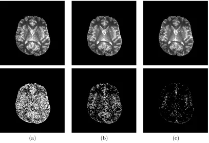
3.5.5 Segmentation of T1-weighted Images . . . 38
3.6 Discussion . . . 41
3.6.1 Registration of Flip-angle Images and Generation of Brain Mask . . 41
3.6.2 Segmentation of Brain Data and Probabilistic Segmentation . . . 41
3.6.3 Joint Segmentation and RF-inhomogeneity Calibration . . . 41
3.7 Conclusion . . . 42
4 Multi-phase Joint Segmentation-Registration and Object Tracking for Layered Images . . . 43
4.1 Introduction . . . 44
4.2 Camera Model and Homographies Between Multi-view . . . 47
4.3 Problem and Strategy Description . . . 51
4.3.1 Algorithm . . . 52
4.3.2 Rough Alignment of Mid-range Layered Images . . . 53
4.4 Multi-phase Active Contour with Joint Segmentation-Registration . . . 56
4.4.1 Joint Segmentation-Registration . . . 56
4.4.2 Adapted to Multi-phase Active Contour . . . 61
4.5 Optical Flow for Object Tracking . . . 67
4.5.1 Tracking in Two Image Sequences Under Constraint . . . 68
4.6 Discussion and Experimental Results . . . 71
4.6.1 MPJSR Results . . . 71
4.6.2 Tracking Results . . . 74
4.7 Conclusion . . . 79
5 Determining Canonical Views of 3-D Object . . . 80
5.1 Introduction . . . 80
5.2 A Model of Sum of Multiple Range Images . . . 82
5.3 MDL-Based Canonical View of a 3-D Object . . . 86
5.3.1 Theory . . . 86
5.3.2 Experimental Results . . . 87
5.4 A Compressive Sensing approach to Canonical View . . . 90
5.4.1 Theory . . . 90
5.4.2 Experimental Result . . . 94
5.5 conclusion . . . 96
6 Contributions and Future Work . . . 97
6.1 Contributions of The Thesis . . . 97
6.1.1 Contributions to Region-based Active Contour for Segmentation . . 97
6.1.2 Brain Segmentation and Accurate T1-Map Generation . . . 98
6.1.3 Joint RF-inhomogeneity calibration and T1-Map Segmentation . . . 98
6.1.4 Segmentation and Registration of Layered Images . . . 98
6.1.5 Canonical Views by Compressive Sensing and MDL Methods . . . . 99
6.2.1 Three-tissue Segmentation . . . 99
6.2.2 RF-inhomogeneity Calibration in the Transverse Plane . . . 100
6.2.3 Change of Phase Number in MPJSR . . . 100
6.2.4 Canonical Views . . . 100
Bibliography . . . 101
Appendices . . . 112
A Derivation of Gradient Flows For Our Proposed Energy . . . 113
LIST OF TABLES
Table 3.1 Different validation metrics for a simulated brain data of T1-weighted
LIST OF FIGURES
Figure 3.1 From left to right the weight βin increases such that the segmented region becomes smaller, and therefore we obtain purer tissues. . . 22
Figure 3.2 A carton illustrating the scanning orientation. . . 28
Figure 3.3 A flowchart for the whole procedure to jointly segment T1-Map and calibrate
RF-inhomogeneity. The procedure includes the registration of flip-angle images, brain mask generation, and our JSRIC method. . . 29
Figure 3.4 JSR technique: two active contours evolve in two flip-angle images (of angles 5◦ and 40◦) to jointly register and segment (generate the brain mask) the brain. The region outside the mask are brightened to better show the contrast. . . 31
Figure 3.5 The T1-Map generated by (a) unregistered and (b) registered flip-angle
images. It can be seen that the anatomical structure of the registered one is clearer than the other. . . 31
Figure 3.6 The error rate E versus number of flip-angles, and 10 flip-angles is at the inflection point of the fitted curve. . . 32
Figure 3.7 The T1-Maps generated by (a)2 (b)6 and (c)10 flip-angles on the top row,
and their corresponding error maps on the second row. . . 33
Figure 3.8 Histogram of a (a) T1-weighted image and a (b) T1-Map. . . 34
Figure 3.9 ”α map”: The plot ofα value versus slice number for two subjects. . . 35
Figure 3.10 . T1-Maps generated from unrectified (First row) and rectified (second row)
flip-angle images at slice number 5, 6, 14 and 15. . . 35
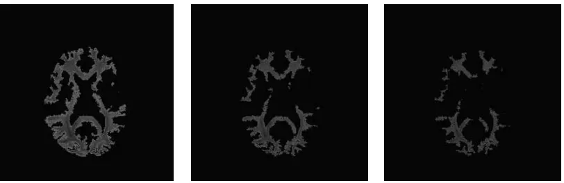
Figure 3.11 . Segmentation result of WM (first row) and GM (second row) for the testing subject at slice number 10 - 13. . . 36
Figure 3.12 Overlap metric of (a) WM and (b) GM segmentations for calibrated and uncalibrated T1-Maps with cubic function G(I) = I3 and tuned weights and also
for calibrated T1-Map with function G(I) =I with tuned weights. . . 37
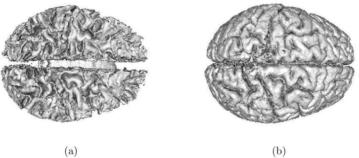
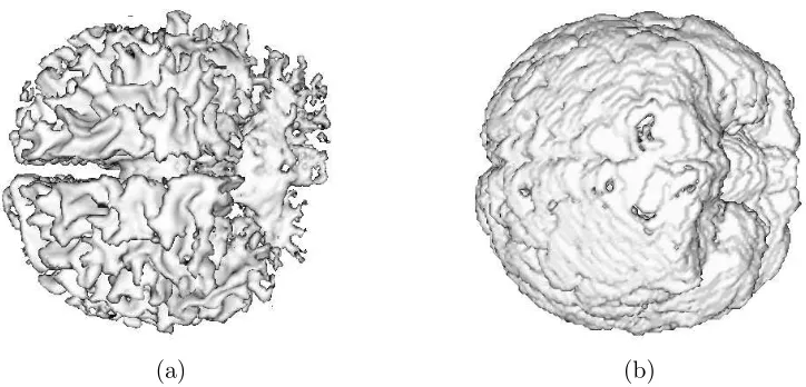
Figure 3.14 3-D segmentation results of (a) WM and (b) GM for the testing simulated brain.. . . 39
Figure 3.15 Average OM for WM and GM segmentations on 20 normal real brain data of T1-weighted modality. The left and right columns denote the average OM of WM
and GM segmentation respectively. Some statistics are from IBSR and others are from [1]. They represent: AMAP: adpaptive MAP, BMAP: biased MAP, FUZZY: fuzzy C-means; MAP: Maximum a posteriori probability, MLC: maximum likeli-hood, TSK-MEANS: tree-structure k-means, FAST: hidden Markov method [2], ZENG: coupled-surface method [3], MPM-MAP: Bayesian method [4],and Dual-front: Dual-front method [1].. . . 40
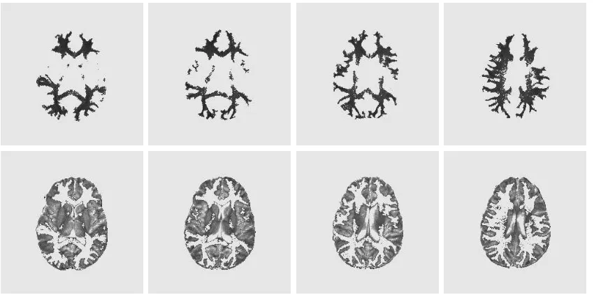
Figure 3.16 3-D segmentation results of (a) WM and (b) GM for one real brain data of T1-weighted modality. . . 40
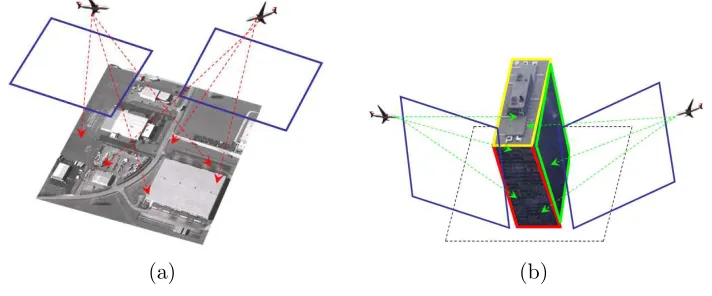
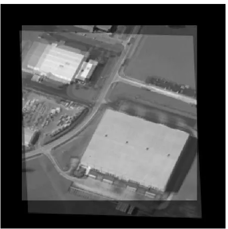
Figure 4.1 (a) Long-range and (a) mid-range layered imaging. . . 46
Figure 4.2 The pinhole camera model. The projected 2-D image is the intersection between the image plane and the rays illuminated from the camera. . . 49
Figure 4.3 Overlayed long-range layered images. One image is affine-transformed and overlapped on top of the other. A single affine transform can bring two images to an almost perfect alignment. . . 49
Figure 4.4 Overlayed mid-range layered images with windows focused on the objects of interest. A single affine transform can only bring two images roughly aligned. . . 50
Figure 4.5 A simple carton explaining our multi-phase joint segmentation-registration and tracking. . . 52
Figure 4.6 3-point correspondence method. 3 points on the basis and reference images are picked up and the affine transformation matrix H can be determined.. . . 54
Figure 4.7 (a.) Simulated images with a square on the left and its affine transformation on the right. The contours successfully segmented both images and captured the registration parameters, (b.) Joint segmentation-registration result for a layered EO image (grey scale image). It captured the front side wall of the building. . . 60
Figure 4.8 3-phase active contour segmentation on a simulated image.. . . 63
Figure 4.10 (Top to bottom) The curve evolution of ternary joint segmentation-registration for two different buildings. . . 72
Figure 4.11 (Top to bottom) The curve evolution of ternary joint segmentation-registration for two buildings which handles topological changes and copes with non-perfect planes.. . . 73
Figure 4.12 (a) The basis image with the located windows overlayed, (b) The transformed objects, which were segmented using ternary joint segmentation-registration, from the basis image will be in alignment with (c) The reference image. . . 74
Figure 4.13 From top to bottom, left to right. The 2 steps of tracking along 10 pair of frames along the layered image sequences. The odd rows show the end of each refinement step, where the contours attached on the boundaries and the registra-tion parameters were obtained; the even rows show the predicregistra-tion step, where the contours were propagated by the calculated velocities. The brighter windows in the even rows denote the new positions of the windows. . . 76
Figure 4.14 From top to bottom, left to right. The 2 steps of tracking along 10 pair of frames along the layered image sequences. The odd rows show the end of each refinement step, where the contours attached on the boundaries and the registra-tion parameters were obtained; the even rows show the predicregistra-tion step, where the contours were propagated by the calculated velocities. The brighter windows in the even rows denote the new positions of the windows. . . 77
Figure 4.15 The brighter contours represent the propagated contours by the calculated velocities, which are closer to the edges compared to the darker contours that are not being propagated.. . . 78
Figure 4.16 The number of approximated planes in the basis image is different from that in the reference image. . . 78
Figure 5.1 example . . . 83
Figure 5.2 example . . . 84
Figure 5.3 (a.) 3-D model, (b.) Reconstructed surface from the 11 canonical views obtained from minimum description length criterion (the poor resolution is due to computational complexity concern). . . 89
Chapter 1
Introduction
1.1
Image Segmentation
For a machine to perceive the world like human beings do, it needs additional
mechanisms to intelligently make sense out of the things it sees. A typical computer vision
system may be described as a systematic structure, in which a real world scene is first
acquired by the sensors (ex: optical lens), possibly followed by a de-noising process (ex:
filters), and a feature extraction procedure. These features are subsequently used for high
levelperception mechanisms, such as recognition and classification.
Segmentation, which detects edge features in images, is found in the middle level
of this hierarchical vision structure. It is a crucial step in the sense that accurate features
extracted in an image will be fatal to a successful recognition process. In addition to
delineating the boundaries of objects in an image, segmentation may also be instrumental
in dividing an image into subregions that separate the objects from the background, or,
discretely, in labeling each pixel as either foreground or background. Not only does it
provide features for later processing, segmentation may help for better visualization or
diagnosis purpose in medical applications or as an essential tool in tracking applications.
Numerous methods were proposed to segment images. Since the pioneering work
of Kass et al. [5], active contours have been extensively used for segmentation. In con-trast to other edge detectors such as Canny [6] or Sobel operators, which may generate
discontinuous and open curves, active contours yield continuous and closed contours. The
functional to be optimized. Minimizing this functional by a gradient descent method drives
the contours to attache onto edges in the imagery. This so-called evolution of the contours is then shown to be governed by a partial differential equation (PDE).
Depending on the type of information the energy functional incorporates, active
contour methods may further be classified into two categories: edge-based [5, 7, 8, 9, 10,
11, 12, 13, 14, 15, 9, 16] and region-based [17, 18, 19, 20, 21, 22, 23, 24, 25, 26, 27] method.
Edge-based methods, such as ”snake” [5] or the geometric active contour [8, 28], stop the
contour movement when an edge is found, which may for example be defined as a high gradient in the image intensity (for a gray scale image). Region-based methods, such as
region competition [19] oractive contour without edges [17, 18], on the other hand examine some statistics (ex: mean or variance) inside and outside the contours. By maximizing
the divergence of the statistics inside and outside the contour, segmentation is achieved.
Region-based methods have been proved to be more robust than edge-based method [19, 18]
and hence are adopted and studied in this thesis. The implementation of a contour evolution
involves the well establishedlevel set method [29], which has at least two advantages: a. it handles topological changes, b. automatically distinguishes the inside and outside region at
any time of the evolution. We will elaborate more about it in Chapter 2. In this thesis we
propose a constrained Mumford-Shah [27] energy functional (Chapter 3) (which falls in the
region-based category), to segment 2-D and 3-D biomedical images. Moreover, we propose a
method, our so-called Multi-phase Joint Segmentation-Registration (MPJSR) (Chapter 4),
to jointly segment and register objects in layered sensing imageries.
Object tracking in videos is also a direct application of segmentation. The simplest
edge-based tracking method is to segment each image in a sequence over time, such that at each frame the objects of interest are depicted. This method does not, however, utilize
any relationship between consecutive frames. A prediction step based on the optical flow (or visual motion) may hence be made to give a good contour initialization at the next
frame [30]. In this thesis we propose a simple tracking method (Chapter 4) for layered
1.2
Relationship Between Segmentation and Registration
Image registration, is the process of finding the correspondence or thetransforma-tion between two images containing the same scene, taken at different times, from different
perspectives, and/or by different sensors, and of overlaying them into one entity. The
purpose of registration may be to align multi-spectral (or modality) images to gain more
information and a better understanding of the scene. The alignment process constitutes the
bottom level of the data fusion hierarchical structure [31]. Different approaches have led
to registration methods being classified into two categories: area-based and feature-based
methods [32]. A feature-based registration method comprises of four steps: 1) feature
de-tection, 2) feature matching, 3) mapping function design, and 4) image transformation and
re-sampling. Segmentation closely relates to registration in the first step. The features
of interest are object boundaries which form the basis for contour evolution. The feature
matching step is addressed by taking into account that the contours are closed curves and
their parametrization along with their variation in multiple images closely followed. In this
sense segmentation is intimately tied to registration, and their interdependence is central
to many applications.
This is manifest in cases where a segmentation technique may not perform well
when using one modality and additional auxiliary information from other modalities (ex:
MRI scans of T1,T2,PD images) is generally beneficial, and the alignment of these modalities
also helps guide the segmentation task.
A joint segmentation and registration (JSR) technique, proposed by Yezzi et al. [33], successfully coupled these two processes in a variational framework. The ratio-nale of this methodology is to basically enforce a relationship (transformation) between two
contours evolved simultaneously in two images by minimizing the sum of their energies.
In this thesis, we adopt the same rationale and further extend it to develop our
Multi-phase Joint Segmentation-Registration (MPJSR) method (Chapter 4), which is
1.3
Motivations and Thesis Contributions
From an engineering point of view, every proposed method or solution comes from
a corresponding real world problem. This thesis, too, is application driven and the novel
segmentation, registration as well as the 3-D model reconstruction methods are proposed to
solve three real and practical problems. We briefly discuss these motivations and describe
contributions in this thesis towards addressing three applications elaborated below.
1.3.1 Brain MRI Image Segmentation
Research work on brain imaging has long been of interest and is challenging. Three
main tissues: GM (Gray Matter), WM (White Matter), and CSF (Cerebrospinal Fluid),
constitute the major parts of the brain. Segmentation of these three tissues is important for
either diagnosis or visualization purposes. The nature of the folded structure of the brain
cortex, the radiofrequency (RF)-inhomogeneity effects of MRI, and the low contrast (ex:
T1-Map) of an image all increase the difficulty for segmentation.
Our first application focuses on T1-Map modality1 with a goal of segmenting this
case of imagery. To that end, several problems need to be studied. They include: a
gen-eration of an accurate T1-Map using a proper set of flip-angle images [34], a registration
between various flip-angle images, a masking to remove extraneous parts and to preserve
the brain structure in the MR images, and a calibration of RF-inhomogeneity. We
pro-pose a constrained Mumford-Shah energy functional which 1) incorporates an
information-theoretic measure of different tissues and 2) puts weights on the various tissues, yielding a
probabilistic approach to segmentation. The proposed functional is driven by a three-tissue
segmentation of the brain. Moreover, the proposed technique simultaneously segments a
T1-Map and calibrates RF-inhomogeneities (our so-called JSRIC method). Our proposed
segmentation method will be demonstrated not only for T1-Map but also for T1-weighted
images, in both 2-D and 3-D settings, and are validated by an expert’s manual
segmenta-tions.
1T
1 (Spin Lattice Relaxation Time) is a time constant in MRI and T1-Map is a parametric map/image
1.3.2 Layered Image Registration and Segmentation
Layered images refer to the images of a common scene taken by (possibly) different
sensors at different altitudes and angles. Examples include aerial views of a city for traffic
monitoring or UAV (Unmanned Aerial Vehicle) airborne image acquisition for surveillance
or target recognition purpose [35]. Our focus differs from that of traditional aerial layered
images at high altitude and making it such that a single affine transformation will align
two images. With sensors located at mid-range altitude, our approach seeks to divide the
image into subregions and to achieve registration for each region, in a divide-and-conquer
fashion.
In this thesis we propose a multi-phase joint segmentation-registration (MPJSR)
technique to segment and register mid-range layered images. Moreover, we introduce an
object tracking procedure between a pair of layered videos to address video sequences. A
constrained optical flow (visual motion) between consecutive frames is calculated to predict
the location of object contours at the next frame.
1.3.3 3-D Model Reconstruction From Multiple Range Images
Range images are images whose pixel value denotes the distance between the sensor
and the object. Range images may be acquired by laser scanners, for example, and may
be so noisy that a 3-D object reconstruction is more than a simple overlay of all the range
images at corresponding positions. A 3-D object reconstruction from multiple range images,
may be viewed as a subsequent step to segmentation and registration. To delineate an object
in a range image requires segmentation and to merge different parts requires the knowledge
of the relative position of each range image, i.e. registration, and the reconstruction of a
3-D object is in this sense a data fusion.
We propose a novel model, for analysis purposes, and for reconstruction of a
3-D object from multiple range images, under the assumption that the segmentation of the
range image is carried out and the scanning angle is known. Moreover, we use the notion
1.4
Thesis Summary and Organization
In Chapter 2 we give a brief review of the theory and background of curve evolution
and segmentation, which will be used throughout the thesis. The curve evolution theory
and its numerical implementation, the level set method [36], are illustrated in Section 2.1.
In Section 2.2, we discuss the two categories, edge- and region-based, active contour
meth-ods for segmentation. Specifically sections 2.2.1 and 2.2.2 give two celebrated examples,
Snakes [5] and geometric (or geodesic) active contour [8, 28] respectively, of edge-based
active contour methods. Section 2.2.3 gives a region-based energy functional and its
corre-sponding curve evolution, which is a special case (piecewise constant approximation of the
image) of the well-known Mumford-Shah model in Section 2.2.4.
In Chapter 3, we propose a constrained Mumford-Shah type energy functional and
a systematic procedure for brain parametric T1-Map segmentation. Based on the proposed
segmentation method we further develop a method to jointly segment T1-Map and calibrate
radiofrequency (RF) -inhomogeneity which is present in all MR scanning processes.
Sec-tion 3.2 details our proposed energy funcSec-tional which incorporates an informaSec-tion-theoretic
point of view along with a weighting to yield a probabilistic segmentation. Section 3.3
first addresses two problems in order to generate an accurate T1-Map: the registration of
flip-angle images in 3.3.1, and the determination of optimal flip-angles in Section 3.3.2. A
systematic procedure for brain T1-Map segmentation is subsequently given in 3.3.3. In
Section 3.4 we describe the model for RF-inhomogeneity calibration in order to generate
an accurate T1-Map and propose our joint T1-Map segmentation and RF-inhomogeneity
calibration (JSRIC) technique. Section 3.5 demonstrates the results of flip-angle image registration, optimal flip-angle determination, the results of JSRIC, and the validation
per-formance. In Section 3.5.5, we further apply our segmentation method on another modality,
T1-weighted data in a 3-D setting, to demonstrate the generality of our proposed model
with validations.
In Chapter 4 we tackle another registration/segmentation problem on layered
im-ageries. Section 4.2 first reviews the camera model to understand our proposed strategy to
jointly segment and register a pair of layered images in Section 4.3. Section 4.4 describes our
proposed multi-phase joint segmentation-registration (MPJSR) technique. We first review
incorpo-rate a multi-phase method in 4.4.2. Section 4.5 extends our MPJSR technique to object
tracking in a pair of layered videos. Section 4.5.1 describes the constrained optical flow (or
visual motion) calculation which is used as a prediction of the contour position in the next
frames. The results of MPJSR are shown in Section 4.6.1, and its application leads to a
successful joint registration and segmentation of a pair of layered images, and an alignment
of the objects of interest in the images. The results of video tracking utilizing optical flow
calculation are shown in Section 4.6.2, which performs well for our methods.
Chapter 5 studies the problem of determining the canonical views from multiple
views of range images. A novel model to reconstruct a 3-D model from multiple range images is first proposed in Section 5.2. Two methods are used to determine the canonical
views. First the canonical views are determined using a MDL (minimum description length)
formulation in Section 5.3 followed by a compressive sensing procedure given in Section 5.4.1,
to parsimoniously sample a 3-D object. The respective reconstruction results are given.
Conclusions and possible directions of future works of this thesis are presented in
Chapter 2
Preliminaries
In this chapter we review the theory of curve evolution, the level set method, and
both of the edge-based and region-based segmentation methods, for the purpose of better
understanding and prelude to subsequent material in later chapters.
2.1
Curve Evolution and Level Set Method
Denote a family of continuous and closed curves by C(s, t) = (X(s, t),Y(s, t)),
which is a mapping I ∈ R×[0, T] 7→ R2, where s parameterizes a given contour and t
parameterizes the family. A general evolution may be expressed as advancing every point
on the curve in an arbitrary direction, written as a combination of the tangent and normal
directions, from an initial position of the contour C0(s)
∂C
∂t =FT(s, t)T +F(s, t)N,
C(s,0) =C0(s), (2.1)
where FT and F are both scalar functions, and T and N respectively denote the unit tangent and outward normal vector. It can be shown [37] that only the normal component
has an effect on the displacement of a point and the tangential component will only affect
the re-parametrization of the curve. Therefore Eq. (2.1) is equivalent to
∂C
Evolving a contour by Lagrangian approach involves the discretization of the
con-tour into finite nodes, and the readjustment of nodes’ spacing after each evolution. This is
required to preserve data fidelity and to reduce numerical approximation errors [38].
Another implicit representation of a contour, the level set function, was proposed
by Osher and Sethian [29] to embed a contour in a one-dimensional higher space to become
a popular scheme for curve evolution. A contour is implicitly embedded in a 0-level of a
level set function, Φ(x, y, t) :R2×[0, T]7→R, as
C ={(x, y) : Φ(x, y, t) = 0},
inside(C) ={(x, y) : Φ(x, y, t)<0},
outside(C) ={(x, y) : Φ(x, y, t)>0}.
(2.3)
While there may be an infinite choices of level set functions, a signed distance function is
preferred for its stability in numerical computations, i.e. Φ(x, y, t) = d((x, y),C), where
d((x, y),C) denotes the Euclidean distance from the point (x, y) to the contour C.
The evolution of the level set function can be derived from the constraint that, at
any time, the contour,C, corresponds to the 0-level set such that Φ(C, t) = Φ(X,Y, t) = 0.
Takeing the partial derivative of Φ with respect to t, we have
Φt+ ΦxXt+ ΦyYt = 0, Φt+ (Φx,Φy)·(Xt,Yt)T = 0,
Φt+∇Φ·Ct = 0, (2.4)
where we have used the subscript to denote a corresponding partial differentiation and ∇
the gradient operator. Substituting the evolution of contour Ct by Eq. (2.2), we have
Φt+∇Φ·F(s, t)N = 0. (2.5)
Notice that the outward unit normal vector can be written as N =∇Φ/k∇Φk [29] where
k · k denotes the Euclidean norm. Replacing it into Eq. (2.5) we have
The forceF(s, t) is often a function of curvature. By letting it equal to the negative curvature, −κ, we have Ct =−κN, or in terms of level set function, Φt =κk∇Φk. This
flow is known as theGeometric Heat Equationand it smoothes an image. It has been shown by Grayson [39] that Heat Equation shrinks an embedded closed curve to a single point
and make it more and more circular along the way. In turns of curve evolution, it also
corresponds to thecurve shortening flow [40] which minimizes the arc-length
L= Z 1 0 ∂C ∂s ds, (2.7)
where we assume C(0, t) = C(1, t). Curvature representation for the level set is κ =
∇ ·k∇∇ΦΦk
, where ∇· denotes the divergence operator, and therefore the geometric heat
flow of the level set is
Φt=∇ ·
∇Φ
k∇Φk
k∇Φk= Φ
2
yΦxx−2ΦxΦyΦxy + Φ2xΦyy Φ2
x+ Φ22
. (2.8)
Notice that in the implementation of Eq. (2.6), the forceF(s, t) is only defined on the 0-level set, or the contour C(s, t) though. We need to define the force on every grid
points in the domain of a level set function for the level set to evolve globally. Different
methods of extending the force, such asglobal ornarrow band extension[29], then follow. To improve on computational complexity, fast implementation such asnarrow band method [41] or real-time method [42] have been proposed as well.
2.2
Active Contour Segmentation Methods
In this section, we review some active contour methods for segmentation. They
can generally be classified into two categories: edge-based and region-based methods. We
present two examples for each category.
2.2.1 Snakes
Kass et al. [5] proposed an energy minimization based framework to deform a contour. The energy can be written as the sum of two terms
whereEint and Eext denote the internal and external energy functionals respectively. The internal energy determines the regularity of the contour such as the smoothness and the
rigidity. A common choice of the internal energy may be given by
Eint=
Z 1
0
α C′(s)
+β
C′′(s)
ds, (2.10)
where α and β are positive reals controlling the weighting between the two terms. The external energy determines the force from the image to guide the contour evolution. A
common choice is to let the edge (high gradient) attract the contour
Eext=
Z
C
1
λk∇Gσ ∗I(x)k
dx, (2.11)
where λ is a real number controlling the weights, and Gσ denotes a smoothing Gaussian filter with standard deviation σ.
In a numerical implementation, finite nodes are used to approximate the contour,
and each node is moved according to some greedy algorithm to minimize the energy. The
resulting contour locates the local minimum ofEs, and if the initial contour is close enough to the boundaries in the image, one hopes the results will reach the global minimum.
2.2.2 Geodesic Active Contour
Caselleset al.[8] and Kichenassamyet al. [28] proposed another edge-based active contour model which is called geometric orgeodesic active contour. The idea of a geodesic active contour is that instead of using a length metric kC′k in the curve shortening flow
(Eq. (2.7)), a new metric which takes into account of the image is used. The model is to
minimize
min
C
Z 1
0
g(∇I(C(s)))C′(s)
ds, (2.12)
where the function g(·) is usually chosen as a monotonically decreasing function of the image gradient to detect edges, such as 1+k∇Ik1 . This new metric therefore does not find the minimal classical length but minimizes a new length definition (g(C)kC′k) which takes
The gradient flow for this model can be derived as
∂C
∂t = (g(C)κ− ∇g·N)N. (2.13)
The geodesic model is also very sensitive to local minima and has to be initialized close to
the edges in order to lock onto the global minimum.
2.2.3 Region-based Active Contour
Instead of examining the image gradient in search of edges, which is very sensitive
to noise, region-based active contour looks at some statistics in the regions inside and outside the contour, and move the contour according to separating these statistics furthest away. Since region-based methods examine the statistics globally of the whole image divided
into subregions, they are proved to be more robust than local edge-based active contour
methods.
Yezzi et al. [18] proposed a global region-based approach that also puts the seg-mentation problem in an energy minimization framework. Let an image consist of two
regions, the foregroundRin and the backgroundRout = Ω\Rin, where Ω denotes the whole domain of the image. An energy functional can be constructed as the difference between
some statistics, for example the mean, of the regions Rin and Rout, and the active contour is evolved in a way to pull these two statistics furthest apart.
min
C Ey(
C) =−1
2(u−v)
2, (2.14)
where u and v denote the mean inside and outside the contour C respectively. When
the active contour locks onto the edges in an image, the energy (2.14) achieves its global
minimum. In other words, this model approximates an image as a piecewise constant
function with its value equal to the means inside and outside the object.
In order to prevent the contour from enclosing outliers such as salt and pepper
type noises, a length penalizing term may be added to yield
min
C E(
C) =−1
2(u−v)
2+αI
C ds, (2.15)
length. The gradient flow of the contour may be derived by calculus of variation to yield
∂C
∂t = (u−v)
I−u |Rin|
+ I−v
|Rout|
N −ακN, (2.16)
where|R|represents the area of region R.
Chan and Vese [17] also proposed a similar energy
min
C ECV(
C) =
Z
Rin
(I−u)2dx + Z
Rout
(I−v)2dx +α I
C ds, (2.17)
and the resulting gradient flow is the same as the flow in (2.16) with the restriction that
the areas inside and outside the contour equal, i.e.,|Rin|=|Rout|
∂C
∂t = (u−v) (2I−u−v)N −ακN. (2.18)
The advantage of these region-based active contours is that they are capable of
zeroing in on the global minimum, regardless of the initialization displaying less sensitivity
to noises compared to edge-based methods.
2.2.4 Mumford-Shah Model
Most active contour methods for segmentation usually find the boundaries which
divide an image into regions assuming that inside each region the intensities are
homoge-neous; most nonlinear diffusion methods smooth an image within homogeneous regions but
not across the boundaries of such regions. Mumfor-Shah’s model [27] simultaneously
ad-dresses these two goals. Their model basically approximates an image by piecewise smooth
functions
E(fRin, fRout,C) =
X
i=in,out
Z
Ri
n
(fRi −I)
2+νk∇f
Rik
2o
dx +α I
C ds, (2.19)
where α, ν ∈ R+ control the weighting between various terms. fR
i approximate
the imageI for regionRi,i∈ {in, out}. fRi is smooth within each regionRi, but not across
the boundaries, and C denotes the region boundaries. By minimizing this functional we
region but not across the boundaries (second term), while penalizing excessive length of
the boundaries (last term). Several papers [43, 44, 45] have addressed the derivation of
an approximated function for Mumford-Shah model, and the results indeed achieved both
Chapter 3
Joint Brain Parametric T
1
-Map
Segmentation and
RF-inhomogeneity Calibration
In this chapter we propose a constrained and novel Mumford-Shah type energy
functional for brain magnetic resonance imaging (MRI) T1-Map segmentation. The
incor-poration of an information-theoretic view and of selective weights achieves better
segmen-tation results, and also makes three-tissue (WM, GM, and CSF) segmensegmen-tation possible.
Based on our proposed method, we propose a joint segmentation and RF-inhomogeneity
calibration (JSRIC) approach to calibrate the RF-inhomogeneity in the vertical (z-) direc-tion and simultaneously segment T1-Maps. In Section 3.2, we review the Mumford-Shah
model for segmentation, followed by an information-theoretic point of view, and then state
our adapted model, with a fast implementation method. In Section 3.3, we study two
prob-lems to generate an accurate T1-Map, by including the registration of flip-angle images and
the determination of optimal flip-angles. We propose a systematic procedure to segment a
brain T1-Map in Section 3.3.3. In Section 3.4, we propose a novel method to jointly segment
a T1-Map and calibrate RF-inhomogeneities of MRI. In Section 3.5, we show the results
of registration of flip-angle images, the optimal flip-angles, segmentation of T1-Maps with
validations, the resulting T1-Map after RF-calibration, and the 3-D segmentations on two
provide some discussion in Section 3.6, and conclude this Chapter in Section 3.7.
3.1
Introduction
Brain structure segmentation is the apportionment of brain tissue into gray matter
and white matter, based on the appearance of tissue in images produced by magnetic
resonance imaging (MRI). Because manual tracing of the boundaries between tissues in the
brain is labor intensive, difficult, error-prone, and unrealistic for large amounts of data,
an automated or semiautomated segmentation technique is needed for either visualization
or diagnosis. Different imaging modalities, such as T1-weighted, T2-weighted, or Proton
Density (PD) images, have been used for different segmentation methods. T1-weighted
images, because of their good contrast [3], have been widely tested for various segmentation
methods [46, 47, 48, 1, 49]. A T1-Map is a parametric image of pure T1 (spin lattice
relaxation time), derived from the solution of an equation describing tissue relaxation,
and a parametric T1 map which is different from a T1-weighted image. The relationship
between T1 and several diseases, such as schizophrenia or sickle cell disease, has been
studied [50, 51, 52, 53], and T1 may be used as a possible indicator of pathology. Change
in T1 of certain voxels in the brain over time, may be be an early indicator of possible
pathology [51]. Therefore, the segmentation of a parametric brain T1-Map may highlight
pathology unseen by other imaging approaches.
Past research has studied the segmentation of cortex in the brain. The three
tissues- white matter (WM), gray matter (GM), and cerebrospinal fluid (CSF), constitute
the main parts in the brain. The goal is to find their respective boundaries. Different
methods have been proposed to achieve this goal, and they may be classified into various
categories: fuzzy segmentation methods [48, 54], Markov random field (MRF) methods [55,
56], Bayesian methods [4], active contour methods [3, 1, 49], or the combinations of two
or more techniques. Some of these combinations are as follows: Leemput et al. [47] used Expectation-maximization (EM) and MRF, Xu et al. [46] used fuzzy segmentation and deformable surfaces, and Zhang et al. [2] combined a hidden Markov random field and an EM algorithm. Our method falls in the active contour category in the region-based
formulation. It is an adaptive version of Mumford-Shah’s model [27] to systematically
Before the segmentation of a T1-Map, several issues arise for obtaining an accurate
T1-Map. A T1-Map may be calculated by a rapid method known as the variable nutation
method [57] which provides comparable precision but much faster speed over conventional
methods [58]. This method requires the acquisition of a set of flip-angle images and the
T1 information can be extracted therein. The problem of determining the set of optimal
flip-angles therefore was studied. Deoni et al. [58, 34] proposed methods to determine the optimal flip-angles by basically maximizing the signal to noise ratio (SNR) of a T1-Map.
Their first work [58] required the knowledge of average TR/T1 in advance though, and
their second work [34] introduced a weighted least-square method to estimate the angles.
We take another approach to determine the optimal flip-angles to achieve the trade-off
between acquisition time and T1 accuracy.
Since a T1-Map is generated by a set of flip-angle images, alignment of of the images
is important in order to obtain an accurate T1-Map. We therefore propose a method to
register the raw data. The registration of flip-angle images is usually ignored though because
the movement of the head in the coil is minute. However, slight registration errors affect
the resulting T1-Map dramatically, as will be shown.
Radiofrequency (RF)-inhomogeneity is another unavoidable problem encountered
in MR imaging. The nonuniform distribution of the RF field can cause the resulting images
to have low contrast and inhomogeneous intensity, which makes quantitative description
and segmentation of the image difficult [59]. The basic theory of MR imaging is that when
the RF field is applied in the scanner and interacts with the magnetic field, the spins of
the protons are tilted by a certain angle (thus the name of a flip-angle image). The spin
returns to the equilibrium state after the RF field is switched off, and the resonance energy
resulting from this return to a fully-relaxed state is what is reconstructed to make the
images [60]. RF inhomogeneity then affects the generation of T1-Map in the sense that the
spins are not tilted by the predefined nominal angles. Hence, we focus on calibrating the RF non-uniformity in order to generate an accurate T1-Map. Cheng et al. [57] calculated
an analytical form of T1errors induced by RF non-uniformity and allowed simple correction
of T1 measurements. Both Wanget al. [59] and Venkatesanet al.[61] incorporate a scaling
factor α to rectify the nominal flip-angles in their models. We propose a method, which assumes the average T1 value among a transverse plane is the same across slices, to jointly
3.2
Proposed Model for Segmentation
Active contour methods comprise a popular segmentation technique in which an
initialized contour is driven by a partial differential equation (PDE) to minimize an energy
functional designed to attract the contour toward image edges. Active contour methods
can be classified into two categories: edge-based [5, 7, 8, 9, 10, 11, 12, 13, 14, 15, 9, 16]
and region-based [17, 18, 19, 20, 21, 22, 23, 24, 25, 26, 27] methods. Edge-based methods
examine the gradient information of the image, and stop the contour whenever the gradient
is high. However, there are many situations when the edge is not clearly characterized
by the gradient, and it has been shown that region-based methods outperform edge-based
methods [19, 26, 17, 18, 23, 25]. By examining some statistics of the region inside and
outside of the active contour, and optimizing the separation of these two statistics, we
may achieve a better segmentation performance, thus making region-based methods more
attractive.
Our proposed model falls in the region-based category. Before stating our adapted
energy, we first illustrate Mumford-Shah’s [27] model. Two adaptations of Mumford-Shah’s
model constitute the novelty of our proposed technique. First is the incorporation of an
information-theoretic view, and second is a selective weighting which favors erring towards
one tissue type or another. Both of them will be illustrated in the following two subsections.
3.2.1 Mumford-Shah Energy and Information-Theoretic View Point
Mumford and Shah [27] proposed an energy functional that models an image as
a piecewise continuous function, i.e., the intensity is homogeneous within the interior and
exterior of the region of an object, but has a jump across the boundaries. Given a closed,
smooth contour C~ located within the image domain Ω, the image can be divided into two regions, the inside and the outside of the contour, Rin and Rout. The energy can then be expressed as
E(fRin, fRout, ~C) =
X
i=in,out
Z
Ri
n
(fRi−I)
2+νk∇f
Rik
2o
dx
+α
I
~ C
where fRi approximates the image I for region Ri, i=in or i=out, and α, ν ∈ R
+ are
parameters that control the relative weighting between various terms above. fRi is smooth
within each region Ri, but not across the boundaries denoted by C~. By minimizing this energy, we search for an approximating function that is faithful to the image (initial terms),
and smooth within the region interior and exterior of the contour (middle terms) but not
across the boundaries, while penalizing excessive boundary length (last term).
In recent work by Unalet al.[23], the authors approach the segmentation problem from an information-theoretic point of view and were able to obtain a general form of the
energy. Rather than pulling some statistics (such as mean or variance) for the inside and
outside region of the contour apart [18], they instead treat the pixel value of the image as
a random variable, and pulled the probability density functions (PDF) of the two regions
apart to achieve the goal of segmentation. They maximized the so-called generalized
Jensen-Shannon (JS) divergence [62], and found that JS divergence corresponds to an energy
EJS =
r
X
j=1
Z
Rin
(uj−Gj(I))2dx
+
Z
Rout
(vj−Gj(I))2dx
, (3.2)
whereGj(·) are some functions of the image, anduj are the expectations ofGj(·),E[Gj(I)]. The constructed function Gj(·) characterizes the property of the PDF of the image. For example it may reflect the degree of skewness or kurtosis of a density relative to a Gaussian
density [63]. A proper choice ofGj(·) will capture the statistical characteristics of the data hence giving a good segmentation.
This energy is actually a generalized form of the external energy functional
pro-posed by Chan and Vese [17], which is a simplified version of the Mumford-Shah energy
with constants in place of the functionsfRin/out. Our first modification of this energy is to
replaceI by G(I) in Eq. (3.1). The choice ofG(·) will be shown in Section 3.5.
3.2.2 Probabilistic Assignment of Segmentation
Our second modification of the energy, which also motivates our method of
seg-menting different brain tissues, is to tune the weights on the inside and outside integrals
prob-abilistic segmentation differs from other probprob-abilistic or fuzzy segmentation [48, 54] in the sense that existing methods yield a measure of confidence in the membership of each pixel
(voxel for 3-D) within a certain tissue class. Our method however works by assigning some
weight, so we have a higher (or lower) chance of segmenting certain kinds of pure tissue. The reason for avoiding a hard segmentation and carrying out either a fuzzy or a proba-bilistic segmentation is because of partial volume effects [46, 1, 3], when some pixels (or voxels)actually contain a mixture of different tissue types.
Our proposed weighting of the inside versus outside energy terms, together with the
aforementioned incorporation of an information-theoretic view, yields the energy functional
E(fRin, fRout, ~C) =
X
i=in,out
βi
Z
Ri
n
(fRi−G(I))
2+νk∇f
Rik
2o
dx
+α
I
~ C
ds, (3.3)
whereβi ∈R+,βin+βout = 1, denote the weights applied on the inside and outside energy terms. This provides a probabilistic assignment to the segmented regions. Enhancing the
weight of the interior of the evolving contour, βin, is tantamount to penalizing both the error of the difference between the approximated functionfRin, and the data fidelity term
G(I), as well as the degree of smoothness of fRin. This would yield a smaller segmented
region which is likely to be more faithful to the image, and of ”purer” tissues. Fig. 3.1
shows examples of white matter (WM) segmentation with different weights. With a larger
inside-weightβin, the segmented region is smaller and the segmented tissues are purer.
3.2.3 Fast Mumford-Shah Implementation
Minimizing the Mumford-Shah energy functional involves solving for the
approxi-mating functionsfRin/out and for the contour C~. The joint search for these infinite
dimen-sional unknowns usually entails gradient descent flows. In particular, the approximated
functions are typically modeled as a linear combination of a basis set whose dimension
equals the number of pixels in the image, i.e. each pixel is assumed to be independent [44].
The curve and the approximated functions are then evolved iteratively along the
Figure 3.1: From left to right the weight βin increases such that the segmented region becomes smaller, and therefore we obtain purer tissues.
method was in order. Alvinoet al.[45] proposed a fast implementation using a significantly smaller basis number to model the approximated functions, while still achieving sufficient
resemblance to the obtained functions when using the pixel-by-pixel basis.
We adopt their so-calledlinear heat equation basis with the change fromI toG(I) to incorporate the statistical properties of the data from an information-theoretic point of
view in Section 3.2.1. We hence have,
fRi = γ1,iG(I) +γ2,imean(G(I)), (3.4)
where mean(·) is the average function, and the coefficients γj,in(out), j = 1,2, may be similarly derived as in [45]. Our derivations are included in Appendix A.
Substituting Eq. (3.4) into Eq. (3.3), and using a classical methods of variational
calculus, the gradient descent evolution of the curve may be derived as
∂ ~C
∂t =
n
βout
h
(fRout−G(I))
2+ν
k∇fRoutk
2i
−βin
h
(fRin−G(I))
2+ν
k∇fRink
2ioN
−ακN, (3.5)
= (βoutFout−βinFin)N −ακN, (3.6)
where κ denotes the curvature of the contour C~, t an artificial time evolution parameter, andN the outward normal of the contour. Fin/out are derived by substitutingfR
in/out from
3.3
Segmentation of a Parametric Brain T
1-Map
A brain parametric T1-Map is not a direct outcome from an MRI scanner but
is actually calculated from several flip-angle images. Because the flip-angle images are
acquired at different times, and because the subject may move during image acquisition,
registration should be carried out first to obtain an accurate T1-Map. Moreover, in order
to achieve a balance between the acquisition time and the resulting T1-Map accuracy, we
propose a method to determine optimal flip-angles. In the following subsections we will
first illustrate how we register the flip-angle images and obtain a mask as a byproduct,
then describe our method to determine a set of optimal flip-angles, and at last describe our
proposed procedure to segment a T1-Map.
3.3.1 Registration of Flip-Angle Images and Generation of Brain Mask
The value of T1is traditionally determined by acquisition methods such as
Inversion-Recovery (IR) or Saturation-Inversion-Recovery (SR). Other rapid methods, such asvariable nutation (the DESPOT method) have been proposed [57], and require acquisition of several flip-angle
images, and calculation of T1. Since these flip-angle images are acquired at different times,
registration must first be accomplished. Even though the interval between consecutive scans
may be as short as two minutes, and movement of the subject’s head inside the receiver
coil may be a few pixels (under the resolution of a 256×256 image), the effects of such
off-registration can be significant, as shown (Fig. 3.5). Here we describe a method to register
flip-angle images and jointly obtain a mask, as a byproduct, to get rid of the skull and other
structures around the brain.
We use a joint segmentation and registration (JSR) technique proposed by Yezzi
et al.[33] with an additional tuning weight, to achieve registration and to obtain the mask. The theory of JSR technique consists of evolving two contours, with a enforced relationship
(ex: rigid or affine transform) between them, in two images according to a partial
differ-ential equation (PDE) which is a result of optimizing, for example, the sum of two energy
functionals.
For our particular task, we may choose a region-based energy, such as Chan and
Vese’s model [17] incorporating weights, which arises as a special case of Eq. (3.3) with
outside the contour. This model approximates the image I by a simple piecewise constant function, which suits our goal here because it creates a mask that divides the image into two
parts- brain region and non-brain region. This uses the data I itself without considering higher-order statistics, and a piecewise constant approximating function is sufficient.
We observe that the boundary between the brain and non-brain is visually more
easily distinguished than the boundary between different tissues within the brain, for every
flip-angle image. For example, Fig. 3.4 shows two flip-angle images, and we notice that the
contrast between the tissues inside the brain is poor. We therefore put a very small weight
βin on the inside energy in Eq. (3.3) to penalize very little the difference between the data inside the contour, I, and the approximated function mean(I). Experimental results show thatβin= 0.4 yields satisfactory results.
Furthermore, our curve evolution is implemented via level-set methods [29] using
the narrow-band techniques [36], where the level set function changes its values only within
a predefined band around the contour. We may therefore initialize a sufficiently small
contour at the center of the images such that it is localized fully inside the brain, and its
evolution will eventually segment only the brain region without crossing the boundary to
the non-brain. We carry out this registration technique pairwise for all flip-angle images,
and once the flip-angel images are registered to each other, they are used to generate a
T1-Map.
3.3.2 Determination of Optimal Flip-Angles
The T1-Map is generated by a variable nutation method which is later detailed
in Section 3.4 for a better understanding of our RF-inhomogeneity calibration method.
We begin by acquiring images at a set of 19 flip-angles which spans the range of standard angles [64] and will give an optimized T1-Map. This is also confirmed by observing that the
generated T1-Map gives the best quality. We call this particular T1-Map thegold standard,
or T1G, and denote this set of angles as ~θ19= [2◦,5◦,10◦,15◦,20◦,25◦,30◦,35◦,40◦,45◦,
50◦,55◦,60◦,65◦,70◦,75◦,80◦,85◦,90◦]. We then compare the T
1-Map generated from all
combinations of the subset of~θ19with T1G. Out of these combinations we select the optimal
subset of angles. Since the data acquisition is slice-based, this study of optimal flip-angle
focuses on the central slice, which is least affected by RF-inhomogeneity [65] and is routinely
corpus callosum, and generally shows the putamen and lateral ventricle [66]. We denote the
optimaln-angles~θopt,n, which is a subset of~θ19, as those that exhibit the smallest difference
between T1G and the T1-Map generated bynflip-angles:
~
θopt,n = arg min ~ θn
X
(x,y)∈brain
T1G(x, y)−T1~θn(x, y)
, (3.7)
where n ∈ {2,3, . . . ,19}, ~θn ⊂ ~θ19, T1~θn denotes the T1-Map generated by ~θn, and the
summation of (x, y) is over the whole brain region at the central slice.
Eq. (3.7) therefore gives 18 sets, with the number of elements ranging from 2 to
19, of optimal angles. For the determination of the optimal set of flip-angles, in reaching
a compromise between acquisition time (efficiency) and T1-Map quality (accuracy), we
examine the error between T1~θopt,n and T1G and compute the error rate. The error rate is
defined as
E = X
(x,y)∈brain
e(x, y)/A(brain), (3.8)
whereA(brain) is the area of the brain, ande(x, y) is the error, defined as 1 if the difference between T1G(x, y) andT1~θopt,n(x, y) is greater than some thresholdε, and 0 otherwise. The
threshold ε is defined as the minimum of the standard deviation among the T1 values of
three brain tissues (WM, GM, and CSF) manually segmented by an expert. The summation
of e(x, y) is over the whole brain at the central slice.
The plot of the error rate versus the number of flip-angles is shown in Fig. 3.6,
where the inflection point of the fitted curve is at 10 flip-angles (~θopt,10 = [2◦,5◦,55◦,60◦,
65◦,70◦,75◦,80◦,85◦,90◦]). We hereafter routinely use these 10 flip-angles to generate the T1-Map, a compromise between efficiency and accuracy.
3.3.3 Brain T1-Map Segmentation Procedure
Once the brain mask is obtained (Section 3.3.1), it is used to segment away the
skull, leaving only three major tissues in the image: WM, GM, and CSF. Notice that
the curve evolution corresponding to the energy introduced in Section 3.2 always results
in a ”binary segmentation”, where we will have regions inside (foreground) and outside (background) the contour(s). We can not simultaneously segment the three tissues, even
weights (Section 3.2.2), to penalize the error between the data term and the approximated
function (Eq. (3.3)) to segment one tissue at a time, with a progression analogous to that
of ”peeling an onion”.
We illustrate our T1-Map segmentation procedure for ahard segmentationof three
tissues, and the probabilistic segmentation is obtained by varying the weights around the
value of the trained weight (Section 3.5.4). This procedure is applicable to both 2-D and
3-D data sets.
A T1-Map segmentation procedure consists of three steps, where the first two steps
are to evolve the contours by minimizing the energy in Eq. (3.3) with different weights, and
the third step is just a simple subtraction. The procedure is: 1) treat WM as the foreground,
everything else as the background, and letβin be the trained weightβin,W M in Eq. (3.3) to segment WM in the interior region of the contour, 2) treat WM and GM as the foreground,
CSF and everything else as the background, and let βin be the trained weight βin,CSF in Eq. (3.3) to obtain CSF in the exterior region of the curve filtered by the brain mask, and 3)
GM is obtained by subtracting WM and CSF from the whole brain. The procedure is based
on the anatomical observation that GM is enclosed by CSF, and that CSF is separated from
WM [47, 3], such that we may peel off one layer at a time.
The choice of function G(I) in Eq. (3.3), which is chosen to better capture the statistical property of T1-Map (and for other modality), will be shown in Section 3.5. The
values of βin,W M and βin,CSF are determined through a training process. Suppose an ex-pert’s manual segmentation is regarded as the ground truth. IfRedenotes the segmentation region by the expert, andRβin denotes the segmentation region by the weightβinwith some
fixed G(I), for some tissue, then the value ofβin,tissue is determined by minimizing
βin,tissue = arg min
βin
1− |Re∩Rβin|
|Rβin|+|Re| − |Re∩Rβin|
, (3.9)
3.4
Joint T
1-Map Segmentation and RF-inhomogeneity
Cal-ibration
RF-inhomogeneity is an unavoidable problem in MR imaging. The strength of the
RF field varies within the MR scanner, such that the resulting image may be of low contrast
or of non-uniform intensity. In what follows, we will first describe how a T1-Map is calculated
from a set of flip-angle images, then how the T1-Map is affected by RF-inhomogeneity and
then show our proposed method to correct it.
3.4.1 Variable Nutation Method with RF-inhomogeneity
A T1-Map is calculated by variable nutation [57], in that images are acquired
using a FLASH sequence at different flip-angles, and T1 is calculated from the slope of a
least-square fitted line to the pair of data hsins(θ)θ,tans(θ)θi, where s(θ) is the signal strength of the flip-angle image expressed as a function of the flip-angleθ.
RF-inhomogeneity affects the computation of T1 in that the spin of protons at
some spatial positions are not tilted by the angle θ because the strength of the RF field is not as predefined. This phenomenon is more prevalent at the periphery of the receiver coil.
Calibration of RF-inhomogeneity can produce a more accurate T1-Map, since this enables
us to correct the flip-angles. Therefore a spatially dependent scaling factor α has to be introduced to adjust the tilted angle [59, 61], i.e. replacingθ byαθ
s(αθ) sin(αθ),
s(αθ) tan(αθ)
, (3.10)
and T1 is extracted from the slope of the line fitted to the above space. Our imaging
set-ting is slice-based across different transverse planes (Fig. 3.2), and since by observation the
RF-inhomogeneity effect is most significant across the z-direction, our proposed joint seg-mentation and RF-inhomogeneity calibration (JSRIC) is as an initial step to easily calibrate
the flip-angles vertically.
3.4.2 Flip Angle Rectification and Segmentation of T1-Maps
Our method is based on the assumption that the ”average” T1 of WM should be
Figure 3.2: A carton illustrating the scanning orientation.
a slice [67], we have no evidence that WM T1 varies within or between slices.
Our joint segmentation and RF-inhomogeneity calibration (JSRIC) method
re-quires first taking the averaged T1 value for segmented WM at the central slice (which is
least affect by RF-inhomogeneity [65]) as the reference, and then iteratively segmenting
and searching for the scaling factor α in Eq. (3.10) for all other slices. This is a three-step iterative process (as shown inside the dashed box on the flowchart Fig. 3.3)
1. Segment WM for thecentral slice by the method proposed in Section 3.3.3, compute the average T1 value of WM, and denote the average asM
2. For slice m, search α by letting it equal αmin+i∆α in Eq. (3.10), and calculate the
corresponding T1-Map, denoted as T1(α). Ifα goes beyondαmax, claim the current
slice as uncalibratable and repeat this step for the next slicem+ 1
3. Segment WM for T1(α), compute the average T1 of WM, and denote it byL(α). If
M 6=L(α), go back to step 2 and increase α (by incrementing i), otherwise claim it is done for the current slice
4. Iterate step 2 and 3 through all the slices
Figure 3.3: A flowchart for the whole procedure to jointly segment T1-Map and calibrate