Two improved methods for mobile robot localization

(1)

University of Windsor University of Windsor

Scholarship at UWindsor

Electronic Theses and Dissertations Theses, Dissertations, and Major Papers

2010

Two improved methods for mobile robot localization

Yuefeng Wang University of Windsor

Follow this and additional works at: https://scholar.uwindsor.ca/etd

Recommended Citation Recommended Citation

Wang, Yuefeng, "Two improved methods for mobile robot localization" (2010). Electronic Theses and Dissertations. 8267.

https://scholar.uwindsor.ca/etd/8267

(2)

TWO IMPROVED METHODS FOR MOBILE ROBOT

LOCALIZATION

by Yuefeng Wang

A Thesis

Submitted to the Faculty of Graduate Studies through School of Computer Science in Partial Fulfillment of the Requirements for

the Degree of Master of Science at the University of Windsor

Windsor, Ontario, Canada 2010

(3)

**1*1**

Library and Archives

Canada

Published Heritage

Branch

395 Wellington Street

Ottawa ON K1A 0N4

Canada

Bibliotheque et

Archives Canada

Direction du

Patrimoine de I'edition

395, rue Wellington

Ottawa ON K1A 0N4

Canada

Your file Votre reference ISBN: 978-0-494-62723-5 Our file Notre reference ISBN: 978-0-494-62723-5

NOTICE:

AVIS:

The author has granted a

non-exclusive license allowing Library and

Archives Canada to reproduce,

publish, archive, preserve, conserve,

communicate to the public by

telecommunication or on the Internet,

loan, distribute and sell theses

worldwide, for commercial or

non-commercial purposes, in microform,

paper, electronic and/or any other

formats.

L'auteur a accorde une licence non exclusive

permettant a la Bibliotheque et Archives

Canada de reproduce, publier, archiver,

sauvegarder, conserver, transmettre au public

par telecommunication ou par I'lntemet, preter,

distribuer et vendre des theses partout dans le

monde, a des fins commerciales ou autres, sur

support microforme, papier, electronique et/ou

autres formats.

The author retains copyright

ownership and moral rights in this

thesis. Neither the thesis nor

substantial extracts from it may be

printed or otherwise reproduced

without the author's permission.

L'auteur conserve la propriete du droit d'auteur

et des droits moraux qui protege cette these. Ni

la these ni des extraits substantiels de celle-ci

ne doivent etre imprimes ou autrement

reproduits sans son autorisation.

In compliance with the Canadian

Privacy Act some supporting forms

may have been removed from this

thesis.

Conformement a la loi canadienne sur la

protection de la vie privee, quelques

formulaires secondaires ont ete enleves de

cette these.

While these forms may be included

in the document page count, their

removal does not represent any loss

of content from the thesis.

Bien que ces formulaires aient inclus dans

la pagination, il n'y aura aucun contenu

manquant.

1+1

(4)

Dedication of Co-Authorship / Previous Publication

I. Co-Authorship Declaration

I hereby declare that this thesis incorporates material that is result of joint research, as

follows:

This thesis also incorporates the outcome of a joint research undertaken in

collabora-tion with Jingxi Chen and Sepideh Seifzadeh under the supervision of Dr. Dan Wu. The

collaboration is covered in Chapter 3 of the thesis. In all cases, the key ideas, primary

con-tributions, experimental designs, data analysis and interpretation, were performed by the

author, and the contribution of co-authors was primarily through the provision of

construc-tive comments.

I am aware of the University of Windsor Senate Policy on Authorship and I certify that

I have properly acknowledged the contribution of other researchers to my thesis, and have

obtained written permission from each of the co-author(s) to include the above material(s)

in my thesis.

I certify that, with the above qualification, this thesis, and the research to which it refers,

is the product of my own work.

II. Declaration of Previous Publication

This thesis includes two original papers that have been previously published/submitted

(5)

Thesis Chapter

Chapter 3

Chapter 3, 4

Publication title/full citation

A moving grid cell based MCL algorithm for

mobile robot localization, The 2009 IEEE

International Conference on Robotics and

Biomimetics (ROBIO 2009)

A dynamic MCL algorithm based on

clustering for mobile robot localization,

The 2010 International IEEE/RSJ Conference

on Intelligent Robots and Systems

(IROS 2010)

Publication status

published

submitted

I certify that I have obtained a written permission from the copyright owner(s) to include

the above published material(s) in my thesis. I certify that the above material describes work

completed during my registration as graduate student at the University of Windsor.

I declare that, to the best of my knowledge, my thesis does not infringe upon anyones

copyright nor violate any proprietary rights and that any ideas, techniques, quotations, or

any other material from the work of other people included in my thesis, published or

oth-erwise, are fully acknowledged in accordance with the standard referencing practices.

Fur-thermore, to the extent that I have included copyrighted material that surpasses the bounds

of fair dealing within the meaning of the Canada Copyright Act, I certify that I have

ob-tained a written permission from the copyright owner(s) to include such material(s) in my

thesis.

I declare that this is a true copy of my thesis, including any final revisions, as approved

by my thesis committee and the Graduate Studies office, and that this thesis has not been

(6)

Abstract

Mobile robot localization is the problem of determining the robot's pose given the map

of its environment, based on the sensor reading and its movement. It is a fundamental and

very important problem in the research of mobile robotics.

Grid localization and Monte Carlo localization (MCL) are two of the most widely used

approaches for localization, especially the MCL. However each of these two popular

meth-ods has its own problems. How to reduce the computation cost and better the accuracy is

our main concern.

In order to improve the performance of localization, we propose two improved

local-ization algorithms. The first algorithm is called moving grid cell based MCL, which takes

advantages of both grid localization and MCL and overcomes their respective

shortcom-ings. The second algorithm is dynamic MCL based on clustering, which uses a cluster

(7)

Dedication

This thesis is dedicated to my parents for their endless support.

(8)

Acknowledgements

My thanks and appreciation to my supervisor Dr. Dan Wu who helps me a lot during

my whole master's study. His encouragement, guidance and support enable me to complete

my research and write this thesis.

I am grateful as well to my external reader, Dr. Jonathan Wu, my internal reader, Dr.

Yung Tsin and my thesis committee chair, Dr. Subir Bandyopadhyay for spending their

previous time reviewing this thesis and giving their valuable comments and suggestions.

Also, I want to thank my friends. They help me solve many difficult problems during

my research.

Lastly, I would like to express my deep and sincere gratitude to my parents, and they

(9)

List of Figures

2.1 The dynamic Bayes network that characterizes the evolution of control,

states and measurements. [10] 9 2.2 Graphical model of mobile robot localization.[10] 12

2.3 Example of grid decomposition over the robot pose.[10] 17 2.4 Example of grid localization in one-dimensional hallway.[10] 18

2.5 Illustration of Monte Carlo localization. [10] 22

3.1 Illustration of the Proposed Method One. (A) Initialization of grid cells, (B) The moving grid cell localization finished, (C) Initialization of particles

after verification, (D) Final result 31 3.2 Cluster Representatives. (A) Point representative for compact clusters, (B)

Hyperplane representatives for clusters of linear shape, (C) Hyperspherical

representatives for clusters of hyperspherical shape.[15] 34 3.3 Illustration of the Proposed Method Two. (A) Initialization of particles, (B)

Part 1 is finished, (C) Part 2 is finished, (D) Localization is finished 39

4.1 NXT main components. (A) Intelligent brick, (B)(C)(D) Motor, (E) Touch

sensor, (F) Sound sensor, (G) Light sensor, (H) Ultrasonic sensor. [33] . . . 41

4.2 NXTRobot.[33] 42 4.3 LEGO MINDSTORMS NXT in our experiment 45

4.4 Environment for the real experiment 45 4.5 Performance of traditional MCL in the real environment 46

(12)

List of Tables

2.1 Bayes Filter [10] 11 2.2 Markov localization [10] 15

2.3 Grid localization algorithm [10] 19

2.4 MCL algorithm [10] 21

3.1 Moving Grid Cell Based MCL 25 3.2 Moving Grid Cell Localization 26 3.3 Verify Grid Cell Localization 28

3.4 MCL algorithm [10] 29 3.5 Dynamic MCL 33 3.6 BSAS Algorithm [29] 35 3.7 MCL algorithm [10] 38

4.1 Proposed Method One Successful Rate (Real environment) 48 4.2 Proposed Method One Successful Rate (Simulated environment) 49 4.3 Proposed Method Two Successful Rate (Real environment 9 = 9cm, r\ =

25%,n = 1/2,1/3,1/4 ) 50 4.4 Proposed Method Two Successful Rate (Simulated environment 0 = 60pixel,r\ =

(13)

Chapter 1 INTRODUCTION

For a mobile robot, it is very important to know its position as most robot's tasks need

the positional information. This is the most fundamental problem in mobile robotics and

known as mobile robot localization problem[l][2][3]. Informally, mobile robot localization

problem is the problem of determining the robot's pose given the map of the environment

and the sensor readings.

There are three kinds of mobile robot localization problems which are characterized by

the type of initial knowledge of its pose: position tracking, global localization, and

kid-napped robot problem[10]. In position tracking the initial pose is known, and the

localiza-tion is achieved by compensating incremental noise in the movement. In global localizalocaliza-tion,

the initial pose is unknown, and it is much more difficult and challenging since the robot

has to determine its pose from scratch. The kidnapped robot problem occurs when the robot

is taken from its current position to somewhere else without being notified the replacement

during the localization process. It is a variant of the global localization which is even more

difficult. In this thesis we mainly focus on global localization.

(14)

local-ization have been proposed, including grid locallocal-ization^], Monte Carlo locallocal-ization(MCL)[l],

and many hybrid approaches. These algorithms represent the uncertainty of a robot's pose

by using probability distributions over the whole space of robot's possible poses instead

of relying on a single best guess[10]. The probabilistic localization algorithms are part

of probabilistic robotics, a research area that represents information using the calculus of

probability theory. Building on the filed of mathematical statistics, probabilistic robotics

endows robots with a new level of robustness in real-world situations [10].

Among all the probabilistic localization algorithms, grid localization and Monte Carlo

localization(MCL) are most widely used, especially Monte Carlo localization. Grid

lo-calization approximates robot's pose in a metric model of environment[7]. The map of the

environment is divided into grid cells, and each grid cell stores the probability that the robot

is in this cell. MCL represents the pose of robot by maintaining a set of particle samples,

which are randomly drawn according to the probability distributions of the robot's pose[l].

1.1 Motivation and Contribution

Grid localization and MCL are two of the most widely used approaches for localization,

especially the MCL. Each of these two popular methods has its own problems. How to

reduce the computation cost and better the accuracy is our main concern. In order to

im-prove the performance of localization, we propose two imim-proved localization algorithms

both of which are extension of MCL. One is called Moving Grid Cell Based MCL which

combines grid localization and MCL, and the other is dynamic MCL based on clustering

which employs a clustering component to reduce the computational cost in the localization

(15)

1.2 Outline

The rest of the thesis is structured as follows.

Chapter 2: Background knowledge. This chapter provides the background

knowl-edge of our proposed methods. First, we will explain the idea of probabilistic robotics, then

the mobile localization problem is discussed. What's more, two main algorithms for mobile

robot localization , grid localization and Monte Carlo localization, are presented.

Chapter 3: Proposed methods. In this chapter, two proposed methods are presented

separately. Details of each method are discussed, also the illustrations of how each method

works are shown.

Chapter 4: Experiment results. In this chapter, experiment results are demonstrated

which show the advantage of both proposed methods compared with traditional MCL. Both

experiments in the real environment of the physical world and simulated environment on

PC are implemented.

Chapter 5: Conclusion and future works. The conclusion of the thesis is given in this

(16)

Chapter 2 BACKGROUND KNOWLEDGE

This chapter provides the background knowledge of our proposed methods. We first review

the basic ideas of probabilistic robotics. Then the problem of mobile robot localization

is introduced. After that we explain the related knowledge about localization. Finally the

most widely used two algorithms for mobile robot localization, grid localization and Monte

Carlo localization, are discussed.

2.1 Uncertainty

By definition, robotics is the science of sensing and acting on the physical world by using

computer-controlled devices[10]. Robotics systems have been widely used in the world

around us and playing an increasing important role. For a robot, it usually consists of the

four main components. (1) a physical body, so it can exist in the real world. (2) sensor, so

it can sense the environment. (3) effector and actuators, so it can act. (4) a controller, so it

can be autonomous [18].

(17)

are caused by a number of factors. First, the environments of the robot are usually

un-predictable especially in the highly dynamic environments such as highways and offices.

Second, the sensors always have their limitations. The range and resolution of a sensor

re-lies on its physical limitations and the noises. Third, the motor used for the robot actuation

is unpredictable. Control noise and mechanical failure always cause uncertainty. Fourth,

the software of the robot may also cause uncertainty as all internal models of the

physi-cal world are approximate. The real world cannot be fully extracted into models. Finally

some uncertainty arises from algorithmic approximations. In a real-time system, accuracy

sometime has to be sacrificed in order to achieve timely response.

As the robot is more and more widely used, uncertainty is becoming a major issue

for the design of robot systems. How to cope with uncertainty is the main concern for

researchers.

2.2 Probabilistic Robotics

Probabilistic robotics is relatively new in the area of robotics which addresses the problem

of uncertainty. The key idea in probabilistic robotics is to represent uncertainty using

prob-ability theory. Instead of a single best guess, probabilistic robotics represents information

by using probability distributions over all possible guesses.[10]

Compared with traditional methods, probabilistic methods have a weaker requirement

on the accuracy of the robot's model, so it prevents the programmer from the heavy

work-load of building accurate models. What's more, probabilistic methods have lower

require-ments on the accuracy of robotic sensors. Building on the filed of mathematical

statis-tics, probabilistic robotics endows robots with a new level of robustness in real-world

(18)

(SLAM)[22], planning[10] and control[10].

2.2.1 State

In probabilistic robotics, the environment is a dynamical system that possesses internal

state. Robots can get information about the environment through sensors and maintain an

internal belief about the environment.

Environments are characterized by state[\0]. It is the collection of the information

about the robot and its environment. State that changes over time such as moving people

around the robot is called dynamic state, while others that remain static such as the location

of a wall are called static state. The state also includes variables about robot itself such as

pose, velocity and so on.

Typical state variables used in robotics are: (1) robot's pose which consists of location

and orientation in a global coordinate. (2) in robot manipulation the state includes variables

for the configuration of the robot's actuators which is often referred to as kinematic state.

(3) robot's velocity and the velocities of its joints, which are usually referred to as dynamic

state. (4) location and features of surrounding object in the environment. An object may

be a wall or a desk, and features may be the visual appearance such as color or texture. (5)

locations and velocities of moving objects and people may be state variables too.[10]

A state is called complete if it is the best predicator of the future. But in practice it is

not possible to get a complete state for a robot system. A complete state not only includes

all aspects of the environment that may affect the future but also the robot itself. Some of

these aspects are very hard to get.

In this thesis, we use x

t

to denote the state at time t and time is discrete, which means

(19)

2.2.2 Environment Interaction

Between the robot and the environment there are two fundamental interactions:

environ-ment sensor measureenviron-ment and control actions[4][10]. The robot can obtain information

about the state of the environment through its sensors, and affect the environment through

its actuators. Examples of the first type of interaction include the camera image or a range

scan. The result of a perceptional interaction is called a measurement. Usually, sensor

measurements arrive have some delay, so they provide information about the state of

cer-tain moments ago. Examples of the second type of interaction include the motion of robot

or manipulation of an object. We assume that the robot always takes control actions even it

does not perform any action itself. In practice, the robot continuously takes control actions

and gets measurements at the same time.

The robot keeps a record of all past sensor measurements and control actions, which

is referred to as the data. Through the two types of interactions , the robot receives two

different data streams, measurement data and control data.

Measurement data gives a robot the information regarding of the momentary state of

the environment. We assume that the robot gets one measurement at one time. The

mea-surement data from time t\ to time ?2 is denoted as z,,

:t2

and the measurement data at time

t is denoted as z

t

. Control data sometimes is also referred to as movement data or motion

data in the context of mobile robot localization problem. We also assume that there is only

one control data at one time, even the robot does not do anything. Control data provides

information about the changes of the state. We use w,,

:f2

to denote the movement data from

time t\ to time ti, and u

t

to denote the movement data at time t.

Both measurement data and control data play very important roles. On one hand,

(20)

robot's knowledge. Control data, on the other hand, brings a loss of knowledge because

of the uncertainly in the real world. One thing needs to be emphasized on is that the sensor

measurement and control actions take place at the same time.

Probabilistic approaches for robotics have two different components to process these

two kinds of data[10]. One is measurement model, and the other is motion model.

Mea-surement model, denoted as p{z.t\x

t

), is the conditional probability of Zt given the state x

t

.

Motion model is the state transition probability p(x

t

\u

t

,x

t

-\). It is the posterior distribution

of x

t

after incorporating the control data u

t

at x

t

- \. This two models are very important for

estimating robot's state.

2.2.3 Probabilistic Generative Laws

The evolution of state is controlled by probabilistic laws. The state x

t

is conditioned

on all past states, measurements and controls, which can be presented in the following

form: p{x

t

\xo-j-\,z\:t-\,u\;

t

)[W\- Here we assume that robot first takes a control

ac-tion u\, then gets a measurement z\. If the state is complete then it is a sufficient

sum-mary of all past events. Particularly, x

t

-\ is a sufficient statistic for all previous controls

(«i:f-i) and measurements (zi

:f

-i) up to time t — 1. So state x

t

could be expressed as

p(xt\xo:t-\ ,zi-j-\ ,u\

:t

) = p(x

t

\x

t

-i,u

t

). The equation is an instance of conditional

indepen-dence, which means if we know the values of the conditioning variables, such a s Xf—\ ]Ufi

then certain variables, such as x

t

, are independent of other variables, such as zut-i and

u\

:t

-\. Also, if x

t

is complete, we will get another important conditional independence:

p(zt\xo:t,z\:t-\,u\

:t

) = p(zt\x

t

), which means the state x

t

is sufficient to predict the

mea-surement data zt, in other words, other variables such as past control data, meamea-surement

(21)

The probability p(x

t

\x

t

-\,u

t

) is called state transition probability, which shows how

state x

t

evolves based on the control data u

t

and the previous state x

t

~\. The

probabil-ity p(zt\x

t

) is the measurement probability which specifies how measurement data z

t

is

generated according to the state x

t

. The state transition probability and the measurement

probability present the dynamical stochastic system where the robot exists. Figure 2.1

illus-trates the evolution of state and measurements. State x

t

is stochastically dependent on the

previous state Jt,_i and the control data u

t

, and the measurement zt depends stochastically

on the state x

t

. The model in Figure 2.1 is well known as hidden Markov model or dynamic

Bayes network[23][24][27].

Figure 2.1: The dynamic Bayes network that characterizes the evolution of control, states

and measurements. [10]

2.2.4 Belief

In this part we will introduce an important concept called belief[\0]. Belief is robot's

internal knowledge with respect to the state. The state usually cannot be measured directly,

so the robot has to infer its belief from the data collected. In probabilistic robotics, belief is

(22)

A belief distribution assigns a probability to each possible state hypothesis with regards

to the true state[10]. The belief at time t is denoted as bel(xt) = p{xt\z\;t,u\:t)- It is a

posterior probability over all possible states conditional on all past control data and all past

measurement data collected so far. Sometimes it is often important to calculate a posterior

after taking the control action ut but before incorporating measurement data Zt, which is

denoted as bel(xt) = p(xt\zut-\,u\:t). This posterior is usually referred as prediction, and it

reflects that bel(xt) predicts state xt based on previous state xt-\ without incorporating the

measurement data zt- Then we also need to calculate bel{xt) from bel(xt) by incorporating

Zt, which is called measurement update.

2.2.5 Bayes Filter

Bayes filter is a recursive algorithm that estimates the state of a dynamical system based on

both measurement data and control data and it is the most general algorithm for calculating

beliefs[l][10]. Table 2.1 shows a single iteration of the Bayes Filter algorithm. As shown

in Table 2.1, the belief bel{xt) is calculated from the previous belief bel{xt-\). The inputs

are the bel(xt-\), control data ut and measurement data Zt• The output is the belief bel(xt).

Bayes filter algorithm is performed in two essential phases, prediction phase (line 2) and

update phase (line 3).

In the first phase, it calculates the belief over state xt by incorporating the control data

ut based on the previous state xt-\. Particularly, we can see that bel(xt) is calculated by

the integral of two probability distributions, the prior assigned to state xt-\ and the

prob-ability that ut causes a transition from xt-\ to x,[10]. This phase is called control update

or prediction phase. In the second phase, it processes the probability that the measurement

(23)

Table 2.1: Bayes Filter [10]

Algorithm Bayes_filter (bel(xt-\, ut,zt)

1: for all xt do

2: bel(xt) — J p(xt\ut,Xt-\)bel(xt-i)dxt-\

3: bel(xt)=T\p(zt\x,)bel(xt)

4: endfor

5: return bel(xt)

However bel(xt) may not integrate to 1, so it uses the normalization constant t| to normalize

the results. The second step is called measurement update or update phase.

Bayes filter needs an initial belief bel(xo) at time t = 0 as an input in order to recursively

calculate the new belief. If the values of XQ is known, then bel(xo) should be initialized with

a point mass distribution which centers all probability mass on the value of XQ, and all the

others are assigned a probability of zero. If the initial value XQ is totally unknown, bel(xo)

should be initialized using a uniform distribution over all possible values of XQ. If the initial

value xo is partially known, then bel(xo) can be initialized by non-uniform distributions.

There is one important assumption called Markov Assumption which is adopted by

Bayes filter. Markov assumption plays a fundamental role in this whole thesis. It assumes

that past and future data are independent if the current state xt is known. It tells that the

current belief bel(xt) is sufficient to represent the past history of robot. In robotics, Markov

(24)

2.3 Mobile Robot Localization

Bayes filter is an important algorithm for state estimation problems, and it has many

ap-plications one of which is mobile robot localization problem. Mobile robot localization

is the problem of determining a robot's pose given the map of the environment and the

sensor readings[10][19]. It is one of the most important problems in mobile robotics as

most robot's tasks need the positional information. In practice, the pose of robot cannot

be sensed directly, so the pose has to be inferred from measurement data and control data.

Also, a single measurement data is usually not enough to determine the pose, so the robot

has to integrate data over time. Figure 2.2 illustrates a graphical model for localization. The

goal of the robot is to determine its position based on the measurements and movements

given the map of the environment. In Figure 2.2, the values of shaded nodes are known

including the map m, the measurement z and the control u. The goal of localization is to

calculate the robot's pose x.

(25)

2.3.1 Category of Localization

From different aspects, localization can be divided into many different categories.

Accord-ing to the nature of environment and the initial knowledge of the robot, here we discuss

four important types of localization problems[10].

Firstly, localization problems can be characterized by the type of knowledge whether

is known at the beginning or at run-time. Under this category, there are three kinds of

localization problems with an increasing difficulty. Position tracking( or local localization)

is the simplest one. The initial pose of robot is known and the localization is done by

accommodating the noise in the robot's movement. The uncertainty of the pose is usually

approximated by a unimodal distribution such as a Gaussian. It is a local problem as the

uncertainty is local and restricted to places near the robot's true pose. In global location,

the initial pose is not known and the robot is placed somewhere in the environment. Global

localization is more difficult than position tracking since it has to determine its pose from

scratch. The third problem is called kidnapped robot problem. It is a variant of the global

localization but more difficult. The robot is kidnapped and taken to somewhere else without

being notified. Kidnapped robot problem becomes important because even the most

state-of-the-art localization approaches can fail sometimes. The ability to recover from failures

is especially important for truly autonomous robots.

Secondly, the environment has a substantial impact on the difficulty of localization[19].

Environments can be static or dynamic. In static environment the only variable quantity is

the robot's pose. All other objects in the environment remain at the same place all the time.

However in a dynamic environment, objects may change its position or configuration from

time to time. Example of changes are like people, movable furnitures and so on. Most real

(26)

environments is more difficult than that in static ones.

Thirdly, according to whether or not the localization algorithm controls the motion,

the localization can be divided into passive localization and active localization[6][17]. In

passive localization, the localization algorithm only observes on the robot's operating, and

has nothing to do with the control of robot. The motion of robot is not designed to facilitate

localization so the robot may move randomly. In active localization, the algorithm controls

the robot in order to minimize the error or cost during the localization. Active localization

algorithms usually produce better results than passive ones.

Lastly, with respect to the number of robots involved the localization can be divided

into single-robot localization and multi-robot localization^] [20]. Single robot localization

is the most studied approach. It handles a single robot only and there is no

communi-cation problems since all the data is collected to a single robot platform. In multi-robot

localization, the robots have to detect each other. The issues that arises usually include

representation of beliefs and the communication between different robots.

In this thesis, we focus on the global passive localization for a single robot in a static

environment.

2.3.2 Markov Localization

Localization algorithms are variants of the Bayes filter. In the context of localization, Bayes

filter is also known as Markov localization[10][19]. Table 2.2 depicts the basic algorithm.

Comparing with Table 2.1, we can see that the difference is that Markov localization needs

the map m of the environment as one input. The map m is very important in the

measure-ment model p(zt\xt,m) (line 3), and is also needed in the motion model p{xt\ut,xt-\,m)

(27)

Table 2.2: Markov localization [10]

Algorithm Markov .localization {bel (xt-\,ut,zt, m)

1: for all xt do

2: bel(xt) = J p(xt\u,,xt-i,m)bel(xt-i)dxx-\

3: bel(xt)=r\p(zt\xt,m)bel(xt)

4: endfor 5: return bel(xt)

bel{xt) at time t from time t — 1 recursively.

Markov localization is able to handle the position tracking problem, the global

localiza-tion problem and the kidnapped robot problem in static environment. In posilocaliza-tion tracking

the initial pose is known, so bel(xo) is initialized by a point-mass distribution. However in

practice the initial pose is often known in approximation, so bel(xo) is usually initialized

by a Gaussian distribution centered around xo- In global localization, the initial pose is

unknown, so bel(xo) is initialized by a uniform distribution over all possible spaces in the

map.

Markov localization is independent of the representation of the state space and it can be

implemented by using different state representation methods, for example, histogram filter

and particle filter.

2.3.3 Representation of State Space

In this part, we will discuss two state representation methods[21], histogram filter[7] and

particle filter[26]. They approximate posterior over continuous spaces with finite values.

(28)

cumula-tive posterior for each region by a histogram which assigns a single probability value to

each region. Particle filter approximates the posterior by a finite number of samples which

populate the state space, and the samples are drawn randomly from the posterior. As these

two methods are well-suited for representing multi-modal beliefs, they are widely used

when a robot has to deal with global uncertainty, such as global localization problem[10].

2.4 Localization Algorithms

Since mobile robot localization is one of the most important and fundamental problems in

the field of mobile robot, so there are a number of probabilistic algorithms proposed for

mobile robot localization. Many of them only address the position tracking problem, such

as Extended Kalman Filter(EKF)[10]. They all employ Kalman filter which is based on the

assumption that the uncertainty of the robot's pose can be represented by a unimodal

Gaus-sian distribution. What's more, they adopt other assumptions such as GausGaus-sian distributed

noise and Gaussian distributed initial uncertainty. Under these assumptions Kalman

fil-ter performs very well for position tracking problem. In global localization problem the

uncertainty of robot needs to be represented by multi-modal distributions, but Karman

fil-ter cannot, so it is not useful when dealing with global localization problem. In order

to overcome this limitation of Kalman filter, Multi-hypothesis tracking(MHT) algorithm

[5]represents the belief of pose by multiple Gaussians, which is mixture of normal

distribu-tions. It can handle the global localization problem, but the computational cost is very high.

However grid localization and Monte Carlo localization(MCL) could handle multi-modal

distribution at a reasonable computational cost which makes them suitable for global

local-ization problem. In the following, we will discuss these two important global locallocal-ization

(29)

2.4.1 Grid Localization

In grid localization[7], it uses a histogram filter to represent the posterior belief over a grid

decomposition of the pose space. Figure 2.3 demonstrates an example of grid

decomposi-tion. The map of the environment is divided into many grid cells. Each grid cell represents

a robot's possible pose in the environment. Each layer represents a different orientation of

the robot, and in this example only three orientations are shown.

Environment

Figure 2.3: Example of grid decomposition over the robot pose.[10]

The algorithm of grid localization is depicted in Table 2.3. Grid cell is denoted as

Xk, and each grid cell is attached with a probability bel{x

t

) = {pk,t}, which stands for the

possibility that the robot is in this grid cell. The notion meanix^) stands for the

center-of-mass of the grid cell JC*. Grid localization is also a recursive algorithm, and in Table 2.3 it

shows a single iteration. It needs the previous value {pk,t-\}, the most recent measurement

data it, control data u

t

, and the map m. It goes through all the grid cells each time and

(30)

U > I , ' , ' , ' , ' , t , t , i , ' , i . i J . J , i , U - . ' , ' , ' , i . ' , ' , ' , 11 > , ' , ' , ' i ' , ' AJ i ' • ' i ' i ' i '•!••,' i ' i T T

bel(x)

'" " " " '" " " ' ii i ii ii i n - r T l l l l l l l ' " • " I

(b) ,1-, 1 , 1 , 1 , 1 , 1 , 1 = 0 3

i l ! ! ! ! ! ! ! !

. i , . . , . . i . . - - t . i • ' , • i. J ••••* i i i

i ' i ' i ' i • i ' i • i • i • i • t I g f n r ' - r

^m^l

1. ' . ' . ' . ' . ' . ' ' ' , ' , ' , ' , ' , ' , ' . ' . T7r~T

i ' f f " "

p(*|x)

~ -*" v--- • ~ *i'4 ;

^:V~

bel(x)

B j ^ Q s s o s J l b a -n-rfirw

(c)

' i ' i ' i '

bel(x)

•w-rfTh-^-rH'iyjl-^- —^rfTH—

(d)

p(ZiX)

b e l ( \ )

^^Ssmaa^A h n II m m

ie) I . I . I . 1 . 1 . 1 , i . i . i i . i 1 . 1 . 1 , . i . M . I i i i i i i i i i i i i i i i i i i i i i i n

r'"T"''r,]"1 r*T''T,'"i"'"i' r'"r'"T

1,l,t,l,1,[,[,l-rt,y l,.r,l„r„T.,t„l„T„l„r

•t..T.,[.,T„l,„[„l„rJ-( I ,. ,l..t.J tl . ,.l ,.l

bel(x)

—~ri~hi—^ n n^-^

(31)

Table 2.3: Grid localization algorithm [10]

Algorithm Grid_Localization({/7^j

1:

2:

3:

4:

5:

for all k do

Pk,t — ]£/V-imotion_model

Pkj = T] measurement-model

endfor

return {pkJ}

_l},«,,Z,,m)

(mean(xk),ut,

(zt,mean(xk),

mean(x

m) /))

updates the probability for each grid cell. Line 2 incorporates the control data and line 3

incorporates the measurement data.

Figure 2.4 shows an example of grid localization in a one-dimensional hallway. In

Figure 2.4 The robot starts without knowing its pose, so the belief is represented by a

uniform histogram. Then in the following pictures, as it moves and senses, some grid cells'

probability values are increasing while some are decreasing.

There are two issues in grid localization. One is the trade-off between the resolution of

grid cells and the accuracy of result, and the state transition problem. The result of the grid

localization depends on the resolution of grid cells. A finer resolution produces a better

result, but also requires greater computational cost. While with a coarse resolution of grid

cells, though the computational cost is reduced, the result may not be accurate. Another

issue is in the motion model when dealing with a high-resolution measurement model and

a coarse-resolution motion model. As only using the center of a grid cell to represent the

grid cell, which in the Table 2.3 is denoted as mean(xk), may lead to a poor result. For

instance, if the robot moves 1 cm/s, and the motion model updates every second, while the

(32)

moves several steps. It will not cause a state transition. A common solution to this issue

is to modify both the motion model and the measurement model by inflating the amount of

noise. However this solution will reduce the information extracted from the measurement.

Similarly we can also inflate the motion model so that the robot can be guaranteed to move

from one grid cell to another even the motion between each update is smaller than the size

of the grid cell. However this may make the robot move faster than commanded, which will

cause more uncertainty in the process of localization.

2.4.2 Monte Carlo Localization

In this part, we will introduce Monte Carlo localization (MCL)[1], one of most popular

localization algorithms. It is easy to implement and works both for position tracking and

global localization problems [10] .

The filter used in MCL which represents posteriors by finitely many samples is known

as particle filter[26], which we introduced in the previous part. MCL represents the belief

bel(xt) by a set x? = {4 ,x) , . . . ,x) '} of M particles over the entire state space, and each

particle denotes a possible pose of the robot. MCL is also a version of sampling/importance

re-sampling (SIR)[11].

The MCL algorithm is depicted in Figure 2.4, and it shows a single iteration. The initial

belief bel(xo) is represented by M particles that are uniformly and randomly distributed in

the whole state space of the environment and each particle is assigned with a weight of

A/- 1, which is called importance factor. In each iteration, MCL algorithm takes as inputs

the previous belief bel(xt-\), movement data ut, measurement data it and the map m of the

environment.

(33)

Table 2.4: MCL algorithm [10]

Algorithm MCL(x? -i,ut,zt,m)

1

2 3 4

5

6 7 8

9

it = Xt = $

for m = 1 to M do

x, = sample_motion_model(M,,xj_|)

w, = measurement-model(z(,xjm ,m)

**&=£+<*!**

m

U!

ml

>

endfor

for m = 1 to M do

draw i with probability a w.

add xy to X/ 10: endfor

12: return X(

(1) Robot motion. Motion model for sample particles is applied in line 3. After each

step of movement, MCL incorporates the movement data u

t

, and from the previous particle

set it generates M new particles that approximate the robot's pose.

(2) Robot measurement. Measurement model is applied in line 4. In this step, sensor

readings are incorporated by reweighting the sample set, during which the weight of each

particle will change.

(3) Important resampling. This phase(line 7-10) is often referred as sequential

impor-tance sampling with resampling. New unweigted particles are drawn from the current

sam-ple set. The probability of drawing a new particle is related to it weight (importance factor).

When the MCL finishes successfully, most particles will converge to a certain area

(34)

Figure 2.5 (a) The robot is globally uncertain about its position and the particles spread all

possible spaces. In Figure 2.5 (b), when the robot reaches the upper left corner of the map,

its belief is still concentrated around four possible locations. In Figure 2.5 (c), finally after

several movements, the robot localizes itself and all particle converge to a small area.

\

Robot position

y

Robot position

(35)

Chapter 3 PROPOSED METHODS

1

3.1 Motivation

As discussed in the background knowledge, the grid localization has two problems: (1) the

trade-off between the resolution of grid cell and accuracy of result and (2) the state transition

problem. For the MCL algorithm, although it is one of the most efficient algorithms for

mobile robot localization, yet it is still able to be improved with respect to efficiency and

computational cost. For that purpose, how to reduce the number of particles and reduce

the computational cost is the key concern. During the past years many algorithms that

extend MCL have been proposed in order to further improve the performance and reduce

the computational cost, such as adaptive samples based MCL approach[12], mixture MCL

approach[14], coevolution based adaptive MCL[13], reverse MCL Approach[9] and so on.

(36)

However combining grid localization and MCL is not well exploited, and few efforts have

been made in incorporating clustering approach into MCL, so in this thesis we propose two

different novel extensions of MCL. One is Moving Grid Cell Based MCL, which combines

grid localization and MCL, and the other is dynamic MCL based on clustering, which

employs a clustering component in the localization process.

3.2 Moving Grid Cell Based MCL

The first proposed method is called Moving Grid Cell Based MCL. It is based on grid

local-ization and MCL, and could solve the problems existing in the traditional grid locallocal-ization

and reduce the computational cost of the whole localization process.

There are three parts of this method: (1) The first part is called moving grid cell

lo-calization part, and in this part the grid cells are used the same way as how particles are

used in traditional MCL. The size of grid cells here is bigger than the size of those used in

traditional grid localization, which makes the the number of grid cells much smaller. We

consider each grid cell as a particle and apply MCL algorithm on these grid cells. Hence,

these grid cells are moveable instead of stationary. So we eliminate the state transition

problem of the traditional grid localization. Since the size of grid cells is big, so we can

only get a coarse pose of robot once MCL algorithm is finished. (2) The second part is

called verification part, we add the verification part in order to verify the result of

mov-ing grid cell localization part. This will help to improve the accuracy of localization. The

verification is achieved through comparing the expected measurement data based on the

previous result with the real measurement data the robot gets. If the difference of these two

data is out of a certain range, then it suggests the accuracy does not meet our requirement,

(37)

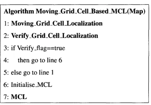
Table 3.1: Moving Grid Cell Based MCL

Algorithm Moving-Grid_Cell-BasedJVICL(Map)

1: Moving_Grid_Cell_Localization

2: Verify _Grid_Cell-Localization

3: if Verify_flag==true 4: then go to line 6 5: else goto line 1

6: InitialiseJVICL 7: MCL

part is traditional MCL part. We apply traditional MCL algorithm to obtain the final pose

of the robot. Instead of in the whole environment, the particles are only initialized in the

restricted area covered by those grid cells produced by the first part. Both the large size of

grid cell in the first part and the restricted area where the particles are initialized in the third

part let us use a smaller number of both grid cells and particles. This helps to reduce the

computational cost. We outline the proposed Moving Grid Cell Based MCL algorithm in

Table 3.1.

As shown in Table 3.1, the algorithm needs the map of the environment as an input. As

mentioned there are three parts of our proposed algorithm, including (1) moving grid cell

localization part (line 1), (2) verification part (line 2-5), and (3) the MCL part (line 6-7).

Line 1 applies the moving grid cell localization algorithm which is shown in Table 3.2. Line

2 applies the verification grid cell localization algorithm which is shown in Table 3.3 . Line

7 applies the traditional MCL algorithm which is shown in Table 3.4. In the following, we

(38)

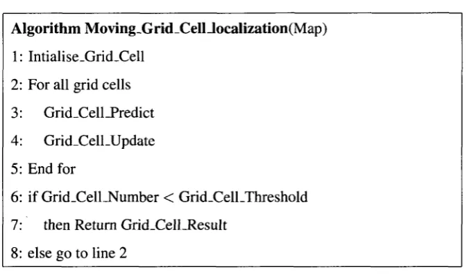
Table 3.2: Moving Grid Cell Localization

Algorithm Moving_Grid_Cell_localization(Map)

1: Intialise-GricLCell

2: For all grid cells

3: Grid_Cell_Predict

4: Grid_Cell.Update

5: End for

6: if Grid_Cell_Number < Grid_Cell_Threshold

7: then Return Grid_Cell_Result

8: else go to line 2

3.2.1 Moving Grid Cell Localization Part

In the traditional grid localization, the number of grid cells is usually very large in order to

get an accurate result. Two factors will affect the number of grid cells. One factor is the

size of the grid cell, and the other is the resolution of orientation. A smaller cell size and

finer resolution of orientation will lead to a more accurate result, however they will greatly

increase the computational cost. In this part, we use a larger size of grid cell and only a

small number of orientation, which makes the number of total grid cells much smaller.

As shown in Table 3.2, we first initialize all grid cells with equal probability that sum

up to 1. We use 3-D representation of the map which includes x-dimension, y-dimensions

and the orientation 8. The way the grid cell used in this part is the same as the particle used

in the traditional MCL algorithm, so the grid cell can be regarded as a big particle. During

the localization process the grid cell is moving like a particle. In line 3 it incorporates the

(39)

with the movement of robot. If the grid is out of the environment, its probability will be

set to zero. Line 4 will incorporate the measurement data and update the probability for

grid cells. Then if the grid cell has a probability of zero, it will be removed from the grid

cell set. As the number of grid cells reduces, when it reaches a certain predefined threshold

according to the map, the moving grid cell localization will stop and return the grid cells

left to the next part, otherwise it will continue.

We use a less number of grid cells and treat them as particles to get a coarse position

in this part, and then in the third part we will get a more accurate position. As the initial

number of grid cells is smaller, the computational cost is reduced. Moreover, during the

process as the number of the grid cells is reducing as the probability of many grid cells are

becoming zero which makes them discarded, so the computational cost is reduced further.

Since we only use a small number of orientations for each grid cell in the part, in the

third part we will compensate for this loss of accuracy in orientation, and we will explain

this in more details in the third part. Because the grid cell is now moving in our proposed

algorithm, the state transition problem existing in the traditional grid localization is avoided.

Therefore, we don't have to worry about the motion model, the robot can move at any

speed. After this first part, only several grid cells are left, the probability that these grid

cells contain the true pose of robot are very high.

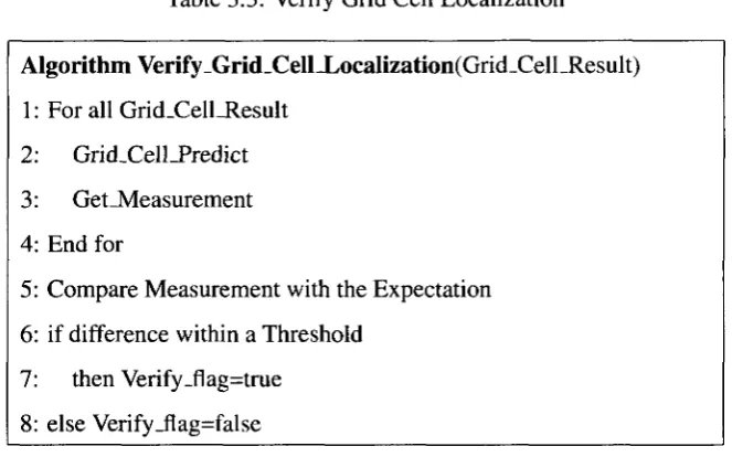
3.2.2 Verification Part

The Verify Grid Cell Localization algorithm is shown in Table 3.3. The input of this

algo-rithm is the grid cells returned in the first part. For each grid cell returned from the moving

grid cell localization part, it will first calculate how long it takes for the robot to reach the

(40)

Table 3.3: Verify Grid Cell Localization

Algorithm Verify_Grid_Cell_Localization(Grid_CelLResult)

1: For all Grid_Cell_Result 2: Grid_Cell_Predict

3: Get_Measurement 4: End for

5: Compare Measurement with the Expectation 6: if difference within a Threshold

7: then Verify_flag=true 8: else Verify_flag=false

to as Expectation in line 5, then it will let the robot move, and record the time the robot

takes to reach the next landmark in the real environment.

If the difference between these two recorded times for each grid cell is within a certain

predefined range, which means the results returned from last part are reliable, then the

verification result will be true, and it will move on and pass the verified grid cell results to

the MCL part. If the difference is out of the predefined range, which means the results from

the first part are not reliable, and the verification result will be false, so it needs to go back

to the first part and go through it again.

The verification part helps to improve the accuracy of localization. When the result

accuracy of the first part does not meet the our requirement, the difference between the

calculated time (Expectation) and the time robot takes in the real environment will be big, so

the algorithm in Table 3.3 will find this out and go back to the moving grid cell localization

(41)

Table 3.4: MCL algorithm [10]

Algorithm MCL(xf - 1 , ut, zt, m)

1 2

3 4 5

6 7

8 9

Xr = it = 4> for m = 1 to M do

x, = sample_motion_model(M,,jc|_j)

w, = measurement-model (zt, x j , m)

- , ^ [ml f/nl ^

endfor

for m = 1 to M do

draw i with probability a w} add x, to X?

10: endfor

12: return %f

What's more, the verification part can be adjusted according to different situations. If

a high accuracy is required, we can make a more complex verification in this part, which

means not only to test the the next landmark, also the second next landmark and so on.

3.2.3 The MCL Part

The third part is the regular MCL part. It is the same as the traditional MCL as shown in

Table 3.4 except how the particles are initialized. From the previous parts we have obtained

a coarse pose of robot , so we only need to initialize the particles in the restricted areas

instead of in the whole environment.

(42)

from the moving grid cell localization part and verified in the second part. The x-dimension

and y-dimension is randomly and uniformly generated inside the grid cells, but the

orienta-tion 6 is generated according to the grid cell's orientaorienta-tion where the particle is in. Because

in the moving grid cell localization part, the orientation of the grid cell is discrete and not

all possible orientations are covered by grid cells, so if the orientation of the robot doesn't

fall into the discrete orientation we choose, the accuracy might be questionable. So in the

MCL part, we initialize the orientation of particles according to the grid cell's orientation,

for example, if the orientation of the grid cell is G, then the orientation of particles in this

grid cell may be between 9—15 and 6 4-15. This will help to compensate the possible

inaccuracy of the orientation in the moving grid cell localization part.

During the process of the MCL algorithm, the probabilities of particles are updated

based on the motion model and measurement model. The MCL goes on until the

localiza-tion is finished. The number of the particles used in this part is not fixed, we can change

the number according to different situations based on the requirement of accuracy.

It is noted that since we already obtain a coarse pose of the robot in the moving grid cell

localization part, then we generate particles only in a restricted area of the environment. We

do not need as many particles as those used in the traditional MCL in which particles have

to be populated in the whole possible spaces.

3.2.4 Illustration of the Proposed Method One

Figure 3.1 shows the progress when executing the proposed method one in a simulated

environment. The big blue circle denotes the robot and the black line denotes the boundary

of the environment. In Figure 3.1 (A) and (B), the colored squares denote the grid cells,

(43)

A

B

D

(44)

Figure 3.1 (A) shows the grid cells initialized in the the first part. Each colored square

denotes a moving grid cell, and in order to make it easy to distinguish each grid cell, the

color of a grid cell is different from its neighbors. Figure 3.1 (B) shows the position of the

grid cell left after the moving grid cell localization part is done. Figure 3.1 (C) shows the

particles initialized after the verification part, and Figure 3.1 (D) shows the result after the

MCL part. Figure 3.1 (D) shows the final position of robot after the whole algorithm is

finished.

3.3 Dynamic MCL Based on Clustering

The second proposed method is dynamic MCL based on clustering. In [16] a novel method

based on clustering is proposed to help robot to be aware of its progress of localization.

Inspired by that, we propose a dynamic MCL which significantly reduces the number of

particles during the execution of localization by employing a clustering component. The

overall structure of the proposal method is shown in Table 3.5.

As shown in Table 3.5, the second proposed method consists of three parts: (1) MCL+BSAS

part (line 1-6), (2) Reducing part (line 7), (3) MCL part (line 8). The four inputs of the

method are the map Map of the environment, the initial particle set % which populates the

whole environment, threshold 0 for distance similarity used in the BSAS algorithm, and

threshold r\ used for termination of the first part. Before we give the detailed descriptions

(45)

Table 3.5: Dynamic MCL

Algorithm Dynamic MCL (Map, %, 6, t|, 1 2 3 4 5 6 7 8

D o {

X,=MCL(Xt-\,ut,Zt) Ct=BSAS(x,,Q)

m = Max(Ct) p = m/Ntotal

} While (p < t | ) Xf =/*«/««? (Xf,n)

MCL (Map, x,')

n )

3.3.1 Clustering and BSAS Algorithm

By definition, a cluster is "an aggregate of points in the test space such that the distance

between any two points in the cluster is less than the distance between any point in the

cluster and any point not in it" [28]. Cluster analysis or clustering is the assignment of a set

of points into clusters.

An important part in all clustering algorithms is to select a proximity measure or

dis-tance measure, which determines how the similarity of two data points is calculated[29].

The proximity measure affects the shape of the clusters, as some elements may be close to

one another according to one distance and far away according to another. In the context

of MCL localization, the pose of a robot consists of x and y coordinates and the accuracy

of localization result has strong relation with Euclidean distance, so it is effective and

rea-sonable that we choose the Euclidean distance d(Pi,Pj) = yj{x-

t

- Xj)

2

+ (y, - yj)

2

as our

proximity measure for two points P, and P

}

when clustering particles.

During clustering in order to calculate the distance d{Pi,Ck) between a particle F, and

(46)

representa-• representa-• . representa-• • • •

(A) (B) CC)

Figure 3.2: Cluster Representatives. (A) Point representative for compact clusters, (B) Hyperplane representatives for clusters of linear shape, (C) Hyperspherical representatives for clusters of hyperspherical shape.[15]

tive of the cluster Q . As shown in Figure 3.2, there are three common options for

rep-resenting the cluster, point representatives, hyperplane representatives and hyperspherical

representatives[15]. In these three methods, the point representative is most suitable for

compact clusters that usually appear in MCL. Therefore, for a cluster containing N

parti-cles, we use the mean point Pmean — ^(Pi) as the representative of the cluster which is a

very common choice.

Many types of algorithms have been proposed in the field of clustering, such as

hierar-chical clustering, partitional clustering, kernel-based clustering, sequential data clustering

and so on[29][31]. Since in the localization we need to process the particles in real time,

so the efficiency of clustering algorithm is very important and crucial for real time

perfor-mance. In our proposed method, we have chosen the sequential algorithm Basic Sequential

Algorithmic Scheme (BSAS)[29][30] due to its simplicity, efficiency, and easy

implemen-tation.

In BSAS, the number of clusters is not required to be known initially. During the

clus-tering process, new clusters are created. Also each particle is presented to the algorithm

only once during clustering.

(47)

Table 3.6: BSAS Algorithm [29]

Algorithm BSAS (xixi---xN),Q)

1: 2: 3: 4: 5: 6: 7: 8: 9: 10

m = l,Cm = {x\}

for / = 2 to N do

find CK : d(x;,Q) = min\<j<md(xi,Cj)

if d(xi,Ck) > 9 then m = m + l,Cm = {x,}

else

Q = Q (J {*/}> update

its representative if necessary end if

: end for

The BSAS algorithm is shown in Table 3.6, X{XI---XN) is the input particle set to be

clustered. For each particle, BSAS either assigns it to an existing cluster or a newly created

cluster, depending on the distance from already formed clusters. The parameter 0 is the

threshold of dissimilarity, which determines how particles are clustered. Line 1 initializes

the first cluster with the first point. Line 2 to line 10 loop through all the data left. Line

3 calculates dissimilarity measures between the current point and every existing clusters to

find a minimum one. From line 5 to line 9, if the minimum measure is larger than 6, a new

cluster will be created, otherwise the current point will be assigned to the existing cluster

which has a minimum dissimilarity measure to it.

In the following part, detailed description of our second proposed method will be

(48)

3.3.2 MCL+BSAS Part

The first part of this method is MCL+BSAS part. In this part, we employ the idea in [16].

This part is iterative and for each iteration, after MCL in line 2, we apply the clustering

algorithm BSAS to the particle set in line 3 so that the BSAS algorithm can provide valuable

information about the distribution of the particles.

As shown in Table 3.5, %t obtained in line 2 is the new particle set after one iteration

of MCL. In line 3, Q is the cluster set which we get after applying the BSAS algorithm to

the whole particle set %,. Variable 6 is used as the threshold in BSAS to decide whether

a particles belongs to an existing cluster or be assigned to a newly created cluster. In line

4, after clustering we could find the cluster with the largest number of particles, and return

the number of particles in this cluster as m. In line 5, the variable p is calculated, and p

is defined as the percentage of m out of the total number of particles (Ntota[). p is used to

evaluate the progress of localization by the MCL algorithm in line 2 and help us keep track

of the convergence degree of particles.

When the value of p exceeds a predefined threshold TJ, the algorithm will assume the

particles have concentrated to a certain degree such that the true robot position is more likely

to be in this cluster which has the largest number of particles. With this newly obtained

knowledge, we do not need to use as many as Ntotai particles for localization and we are

ready to reduce the number of particles for the rest of the localization process. Then the

algorithm will go to part two, the reducing part.

3.3.3 Reducing Part

In this part, we will reduce the number of particles and generate a new set of small number