Analysis of plant-wide disturbances through data-driven techniques and process understanding

Full text

(1)15 th IFAC World Congress 2002, Barcelona. Paper 1306. ANALYSIS OF PLANT-WIDE DISTURBANCES THROUGH DATA-DRIVEN TECHNIQUES AND PROCESS UNDERSTANDING Nina F. Thornhill+, Chunming Xia*, John Howell*, John Coxx and Michael Paulonisx +Department of Electronic and Electrical Engineering, Torrington Place, University College London, London WC1E 7JE, UK (corresponding author). *Department of Mechanical Engineering, University of Glasgow, Glasgow, Scotland. x Eastman Chemical Company, Kingsport, TN, USA. Abstract: Plant-wide disturbances can have an impact on product quality and running costs. Thus there is a motivation for automated detection of a plant-wide disturbance and for diagnosis of the root cause. In this article, data-driven techniques are used to analyze plant-wide disturbances caused, for instance, by limit cycle oscillation in a control loop. The control loops participating in the disturbance are detected and displayed on a process schematic. Other numerical signatures derived from the data trends are utilized for the diagnosis of the root cause. The outcome is a visual display that integrates process understanding and data-driven analysis. Key words: Chemical industry; control loop performance; diagnosis; non-linearity; plant-wide disturbance; power spectrum; process control; self validation; surrogate data.. statuses determined were as itemized below. The illustrations given here are process effects although sensor faults such as bias or drift were also considered: • Steady; • Compensated: a small or slow disturbance handled by a move in the controller output; • Short term transient: a short-term large disturbance; • Long term transient (non-cyclic): a non-stationary disturbance; • Long term transient (cyclic, including ultimate cyclic): a valve problem, limit-cyclic disturbance, bad tuning; • Critical: a change in the process such that controller settings are no longer valid. An overall figure of merit was also determined. Xia and Howell (2001c) combined several single number statistics to form an index, OLPI (Overall Loop Performance Index), to isolate a problem loop in a number of interacting loops. The value of the OLPI. 1. INTRODUCTION The detection and diagnosis of plant-wide disturbances is a key issue facing the process industries (Qin, 1997). Oscillations are a common type of plant-wide disturbance and the detection and diagnosis of oscillatory behavior in a chemical process is of importance because process variability has an impact on profit. In this paper, the previous work of the authors on loop status statistics and plant-wide disturbance detection has been extended to improve the overall outcome. The approach is demonstrated by analyzing industrial case study data provided courtesy of Eastman Chemical Company. The status of a control loop has been examined by Xia and Howell (2001a), who used a comparison of the signal to noise ratios of controlled variable and controller output. Their concept was of self validation in which the controller would determine and display its status in real time by means of an icon in the plant schematic (Xia and Howell, 2001b). The. 1.

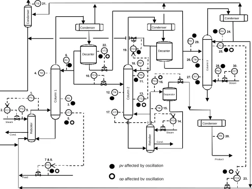
(2) Off-line diagnosis of a root cause was accomplished using a signature for non-linearity that grows stronger closer to the source (Thornhill et. al, 2001b). The non-linearity test determines whether a time series could plausibly be the output of a linear system driven by Gaussian white noise, or whether its properties could only be explained as the output of non-linearity (Theiler et. al., 1992; Kantz and Schreiber, 1997; Schreiber and Schmitz, 2000). The test statistic used was the r.m.s. value of the error from non-linear prediction using matching of nearest neighbors in an m − dimensional phase space (for instance, a plot of x(n) versus x(n − d ) for some delay d would be a two dimensional phase space).. reflects the extent of control efforts the controller provides. The root cause loop would have a larger OLPI value than others. The definition of OLPI is given by: OLPI = LL * max(η y , η u ) / γ , where LL is filtered value of Loop Status, η y and η u are indices estimated from controlled variable (y) and controller output (u) of a control loop, and γ is a threshold value of the indices (Xia and Howell, 2001c). The off-line detection of oscillatory plant-wide disturbances has been demonstrated by Thornhill et. al., (2001b), who inspected the regularity of the zerocrossings of autocovariance functions of the measurements of the process variables (pv) and provided an automated means of grouping oscillations with similar periods. The method also determined the percentage spectral power associated with the oscillation: for example, 100% power in an oscillation would mean there were no other oscillations present in the measurement and no noise.. Finally, root cause diagnosis requires a knowledge of the process because it is necessary to explain the means by which a plant-wide oscillation propagates. 21.. Condenser. TI3. An extension proposed here is to also apply the methods of oscillation detection and non-linearity analysis to the controller outputs (op) and the set points (sp) of the ‘inner loop’ controllers. The complementary contributions of the various signatures to an overall analysis are discussed.. Condenser Condenser. Condenser. FI4. FI3. 22.. TI2. FC5. FC4. 26.. TI5. 27.. FC3. PI1. TI4. TI1. PC2. 17.. 15.. LC3. FC6. Condenser. FI5. FC1. 20.. Cond.. 7 & 8.. Feed. 14.. Steam. Reboiler. Cond.. TI7. Separator. 5. Steam. FC7. Steam. 13.. 3. LC1. 30.. PI2. TC1. TI6. 9.. 28.. 16.. Reboiler. 2.. 12.. Column 2. Column 1. 11.. 1.. TI8. FI2. Column 3. 18.. 10.. PC1. 25.. Decanter. Decanter. FI1. 4.. 29. TC2. 19.. LC2. 6.. 24.. Product. pv affected by oscillation op affected by oscillation. Fig. 1. Process schematic. The circular symbols show the tags affected by a plant-wide oscillation.. 2. FC8. 23..

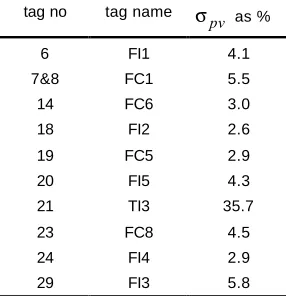
(3) from the proposed root cause to other tags. It is shown that process understanding and the process schematic allowed a root cause diagnosis to be achieved.. seen that the disturbance affects column temperature causing variability in the product composition. The disturbance also affects column loading in a periodic way, limiting production rate. Therefore there is an incentive to determine the cause of the variation and to fix it. The purpose of the analysis in this paper is to determine the extent to which each control loop and indicator participates in the plant-wide oscillation and to find the root cause. It is noted that there were also other oscillations present. For instance, there was a fast oscillation with a period of about 6 minutes in some tags such as 15 (TI6). The focus here is on the slower plant-wide oscillation with a period of nearly two hours because it was a prominent and widespread disturbance.. Section 2 of the paper introduces the industrial process. Sections 3 and 4 discuss the detection and diagnosis of a plant-wide oscillatory disturbance and show how knowledge of the process schematic enhanced the data-driven methods. The paper ends with conclusions and recommendations. 2. THE INDUSTRIAL PROCESS 2.1 The process Schematic: The process schematic is shown in figure 1. The process features three distillation columns, two decanters and several recycle streams. There are 15 control loops and 15 indicators which are numbered from 1 to 30 on the schematic. Six of the eight flow controllers are in a cascade configuration, therefore their set points (sp’s) as well as the process variables (pv’s) and controller outputs ( op’s) are time varying.. 3. DETECTION OF PLANT-WIDE OSCILLATION 3.1 Loop status monitoring Loop status monitoring was designed for real-time use. For the purposes of this paper the loop status tests were run as if on-line by making use of a moving window in the data. The method targeted stand-alone loops and the master controllers in a cascade. Table 2 summarizes the status of loops.. Table 1. Plant variability statistics tag no. tag name. σ pv as %. 6. FI1. 4.1. 7&8. FC1. 5.5. 14. FC6. 3.0. 18. FI2. 2.6. 19. FC5. 2.9. 20. FI5. 4.3. 21. TI3. 35.7. 23. FC8. 4.5. 24. FI4. 2.9. 29. FI3. 5.8. Table 2. Loop status and OLPI indexes. tag no. tag name. loop status. OLPI. 5. LC1. long-term transient (cyclic). 14.3. 13. TC1. long-term transient (cyclic). 38.4. 22. LC2. long-term transient (cyclic). 132. 25. TC2. long-term transient (cyclic). 13. 30. FC7. compensated. 7. Loops 5 (LC1), 13 (TC1), 22 (LC2) and 25 (TC2) were all diagnosed in the category long-term transient (cyclic). It can be concluded that on-line implementation of the loop status monitoring tool would detect the presence of the plant-wide oscillation with a period of two hours.. Data set: Uncompressed data were sampled from the control system every 20 seconds for each of the indicators and for the setpoint, measurement, and output of the control loops. Figure 2 shows the measurements (pv’s) from two days of running for all 30 plant tags. Figure 2 also shows the controller outputs (op’s) for the tags that are under automatic control. All time trends were scaled to unit standard deviation.. Tag 30 (FC7), with compensated status, was subject to a unique disturbance that will be relevant to the understanding of the analysis and will be discussed later.. Table 1 lists the tags whose pv’s were varying by more than 2% (i.e. where σ pv > 0.02 × pv where pv. 3.2 Analysis and characterization of oscillations The analysis and characterization of oscillations is a plant-auditing exercise. The audit was conducted offline and therefore complemented on-line loop status monitoring which highlighted the presence of a problem requiring investigation. The loop status test utilized the controller output (op) as well as the pv. Therefore oscillation detection and non-linearity. is the mean value and σ pv the standard deviation of the pv). Visual inspection of the time trend plots in figure 2 shows the presence of oscillations with a period of nearly two hours (113 minutes or about 340 sample per cycle). The oscillation affects many pv’s and op’s and is therefore a plant-wide oscillation. It can be 3.

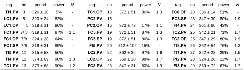
(4) analysis were applied to the controller outputs and also to the set points of inner loops of a cascade.. 4. DIAGNOSIS OF PLANT-WIDE OSCILLATION. Automated oscillation analysis confirmed the presence of the oscillations that can be seen in figure 2 and evaluated the power associated with the oscillation. A tag was judged to be participating in the plant-wide oscillation if it had more that 5% of its spectral power associated with the oscillation. The period was about 340 samples per cycle or 113 minutes. It was shared by the tags highlighted in Table 3 at the end of the paper. The tables gives oscillation period (if any) in the pv and op, and shows the percentage power associated with the oscillation, which was close to 100% in some cases. The high power indicates that finding the root cause of the oscillation would address much of the variability present in this plant. A comparison of Tables 2 and 3 shows that the online loop status test successfully highlighted the controllers having high power oscillations.. 4.1 Non-linearity testing Many authors have described the problems caused by non-linear valve faults such as dead-band and stiction. The resulting limit cycle oscillations are a common cause of plant-wide oscillation (Ender, 1993; Hägglund, 1995; Ettaleb et. al., 1996; Taha et. al., 1996). When the root cause of an oscillation originates in a valve non-linearity the time trends of measurements closest to the fault are the most non-linear. The reason for this is that process dynamics provide mechanical low pass filtering of the time trend and remove the non-linearity from measurements further from the root cause. Therefore the root cause may be sought in the area of the plant where the non-linearity is highest. The non-linearity was determined from samples 1000 to 5000 (5.5 to 27.7 hours) where the oscillations were well established. Table 3 gives the non-linearity indexes for cases where non-linearity was detected. A dash means no non-linearity was detected. The uncertainty in the index is about ±0.12. Thus, for instance, it is not possible to say that Tag 19 (FC5) was really more non-linear than Tag 13 (TC1) but it is certain that both had some non-linearity.. normalised pv. normalised pv. 1 2. 16 17. 3 4 5 6 7. 18 19 20 21 22. 8 9 10 11 12 13. 23 24 25 26 27 28. 14 15. 29 30 0. 8. 16. 24 time/hours. 32. 40. 48. 0. 8. 16. normalised op 16 17. 3 4 5 6 7. 18 19 20 21 22. 8 9 10 11 12 13. 23 24 25 26 27 28. 14 15. 29 30 8. 16. 24 time/hours. 32. 40. 48. 32. 40. 48. normalised op. 1 2. 0. 24 time/hours. 32. 40. 48. 0. 8. 16. 24 time/hours. Fig. 2. Normalized time trends of pv and op of 15 controllers and pv of 15 plant instruments. 4.

(5) 4.2 Application of process understanding. upstream. Likewise no mechanism exists for TC1 to influence LC2. The uneven flow of FC5 (Tag 19) might disturb the flow from the bottom of its decanter but it could not upset the level LC2 because flow from LC2’s decanter is controlled.. Plant-wide oscillation Figure 1 shows the distribution of the plant-wide oscillation on the process schematic. The filled symbols indicate where the oscillation appeared in the pv and the open symbols show control loops where the oscillation appeared in the op. The schematic indicates that many plant measurements were affected by the oscillation and where the measurement would be affected if it were not under control. For example, the oscillation was removed effectively by controller of PC2 (tag 16) because its pv was not oscillating but the op was oscillating.. Discussion: Figure 3 show the signal flows between the major controllers for the proposed root cause in the control valve of LC2 (Tag 22). The figure compares OLPI, total power and non-linearity. The OLPI and total power in the oscillation diminish further from LC2. The results therefore show that total power in the oscillation and the OLPI are signatures that grow stronger closer to the root cause.. Root cause reasoning: OLPI was highest for Tag 22 (LC2) and the percentage power associated both with pv and op was highest for LC2.. The non-linearity index generally decreased in the TC1 and FC5 branch but not in the TC2 and FC8 branch. Non-linearity is generally expected to diminish further away from the root cause. The reason why non-linearity did not reduce as expected is because there is a second source of non-linearity in column 3.. LC2 was among a group of oscillating tags that showed non-linearity in their time trends. The nonlinearity was highest in the tags associated with column 3 and with LC2 itself. Non-linearity was present also in column 2.. Figure 2 shows the steam flow Tag 30 (FC7) was disturbed by asymmetrical randomly-arriving transient events which propagated to PI2, TI7, TI8 and TC2 and FC8. The non-linearity index of the steam flow was 1.3 and therefore the non-linearity of tags in column 3 was higher than expected.. Therefore the control valve of LC2 is a candidate for the root cause because its OLPI was largest, the power of the oscillation was largest and it was in a group of non-linear tags. Mechanisms of propagation: The process schematic shows that a mechanism exists for disturbances from Tag 22 (LC2) to propagate to all the other tags, as follows: • Uneven flow through the control valve of LC2 would affect Tag 29 (FI3) and propagate to column 3 including Tag 25 (TC2); • Disturbance to Tag 25 (TC2) would propagate to the cascade controller FC8 (Tag 23) and upset the recycle flow to column 1, and hence disturb the level controller LC1 (Tag 5). • LC1 would adjust FC1 (Tags 7 and 8) to compensate for the disturbance to the recycle flow. It can be seen from Figure 1 that FC1 (Tags 7 and 8) and FC8 (Tag 23) are almost in antiphase; • It is less obvious how uneven flow through the control valve of LC2 would upset column 2 since the feed (FC4, Tag 10 ) was not affected by the plant-wide oscillation and neither was the reflux (FI2, Tag 18). It is likely that the feed or reflux composition varied because of disturbances to one or both decanters; • Disturbance to FC5 also propagated to LC1 and FC1 through the recycle, as described above for the FC8 recycle stream.. 22. LC2. OLPI = 132 P = 97% N = 1.6. 13. TC1. OLPI = 38 P = 90% N = 1.2. 25. TC2. OLPI = 13 P = 71% N = 1.7. 19. FC5. OLPI = P = 87% N = 1.3. 23. FC8. OLPI = P = 87% N = 1.9. OLPI = 14 5. P = 82% LC1 N < 1. OLPI = 7&8. P = 87% FC1 N < 1. Fig. 3. Propagation from the proposed root cause to other controllers in the plant. 4.3 Confirmation of the root cause The time trends associated with the control valve for LC2 were investigated. The flow through that valve was not measured but FI3 (Tag 29) was equal to that flow plus material from the decanter for column 2. Therefore FI3 was used as a proxy for the flow through the control valve for LC2.. Other hypotheses can be ruled out because no mechanism exists for their propagation. For instance loop TC2 could not be the root cause. TC2 influences recycle from column 3 to column 1 through the action of the FC8, and could disturb TI7 and TI8. However, it could not disturb FI3 because the feed to the column is determined only by conditions. 5.

(6) Figure 4 shows the valve demand (the op from LC2) versus the flow through the valve (FI3) and also plots their time trends. The valve has the signature of a deadband because FI3 tends to stay at a constant value whenever the valve demand changes direction.. methodology provides a foundation for future refinement such that a human would be involved later and later in the diagnostic process. ACKNOWLEDGEMENTS Nina Thornhill and Chunming Xia gratefully acknowledge the financial support of the Royal Academy of Engineering (Foresight Award) and the Committee of Vice-Chancellors and Principals (ORS Award). The project was also supported by the Natural Science and Engineering Research Council (Canada), Matrikon (Edmonton, Alberta) and the Alberta Science and Research Authority through the NSERC-Matrikon-ASRA Industrial Research Chair in Process Control, director Sirish Shah.. It is well known that a valve with a dead band can cause persistent limit-cycle oscillation. These results thus indicate that the cause of the plant wide oscillation with a period of two hours was the valve in the LC2 level control loop. This diagnosis was confirmed following testing on the control valve of LC2. When LC2 was put in manual for the test the plant-wide oscillation disappeared. The valve has been scheduled for maintenance at the next shut-down.. REFERENCES Ender, D.B. (1993). Process control performance: Not as good as you think. Control Engineering (Sept), 180-190.. FI3.PV. Ettaleb, L, M.S. Davies, G.A. Dumont, and E.E. Kwok, (1996). Monitoring oscillations in multiloop systems , IEEE Int. Conf. Cont. Appl., 859-863. LC2.OP. Hägglund, T. (1995). A control-loop performance monitor. Control Eng. Practice, 3, 1543-1551. Kantz, H. and T. Schreiber (1997). Nonlinear time series analysis. Cambridge University Press, Cambridge, UK.. LC2.OP. Qin, S.J., (1998). Control performance monitoring - a review and assessment, Comput. Chem. Eng., 23 173-186.. FI3.PV. Schreiber, T., and A. Schmitz (2000). Surrogate time series. Physica D., 142, 346-382. 6. 8. 10. 12. 14. 16. Taha, O., G.A. Dumont, M.S. Davies (1996). Detection and diagnosis of oscillations in control loops. IEEE Conf. Decision and Control, Kobe, Japan, 2432-2437. Theiler, J., S. Eubank, A. Longtin, B. Galdrikian, B., J.D. Farmer (1992). Testing for nonlinearity in time-series - the method of surrogate data. Physica D, 15, 77-94. Thornhill, N.F., S.L. Shah, and B. Huang (2001b). Detection of distributed oscillations and root cause diagnosis, Preprints of CHEMFAS-4, IFAC, 167-172.. time/hours. Fig. 4. Diagnosis of valve deadband. 5. CONCLUSION This paper has shown how process data, a toolkit of data analysis techniques, and process understanding can be utilized to detect disturbances that propagate plant-wide and to identify their root causes. Application to an industrial process found the root cause for a disturbance affecting nearly all the controllers and indicators in the process. At present, human interaction is required to aggregate and filter the analysis results using process understanding to make the diagnosis of root cause. The benefit of the methods are that the human interaction is with a small number of information-packed statistics. The. Thornhill, N.F., B. Huang, and H. Zhang (2001a). Detection of multiple oscillations in control loops, J. Process Control, accepted. Xia, C., and J. Howell (2001a). Controller output based, single number statistics for loop status monitoring, Preprints of CHEMFAS-4, IFAC, 127-134. Xia, C., and J. Howell (2001b). Loop Status Statistics, Preprints of CHEMFAS-4, IFAC, 372-376. Xia, C., and J. Howell (2001c). Control Loop Status Monitoring, submitted to Journal of Process Control.. Table 3. Characterization of plant-wide oscillation with average period of 340 samples per cycle tag. no. period. power. N. TI1.PV. 3. 326 ± 10. 5%. -. LC1.PV. 5. 320 ± 24. 82%. 5 319 ± 31. 86%. LC1.OP. no. period. power. N. period. power. N. TC1.OP. 13. 372 ± 51. 86%. 1.3. FC8.OP 23. 336 ± 14. 51%. -. -. PC2.PV. 16. -. -. -. FC8.SP 23. 347 ± 30. 80%. 1.9. -. PC2.OP. 16. 373 ± 72. 17%. 1.1. FI4.PV 24. 361 ± 66. 43%. -. 372 ± 51. 87%. 1.3. TC2.PV 25. 342 ± 21. 71%. 1.7. tag. tag. no. FC1.PV 7/ 8. 319 ± 31. 87%. 1.1. FC5.PV. 19. FC1.OP 7/8. 324 ± 28. 64%. -. FC5.SP. 19. 372 ± 51. 86%. 1.3. TC2.OP 25. 347 ± 29. 80%. 1.9. FC1.SP 7/8. 318 ± 31. 89%. -. FI5.PV. 20. 312 ± 102. 15%. -. TI8.PV 26. 362 ± 54. 76%. 1.3. TI5.PV 11. 315 ± 53. 56%. -. LC2.PV. 22. 362 ± 36. 97%. 1.6. TI7.PV 27. 322 ± 22. 29%. 1.5. TI4.PV 12. 374 ± 69. 90%. 1.3. LC2.OP. 22. 359 ± 20. 98%. 1.7. PI2.PV 28. 324 ± 26. 22%. 1.7. TC1.PV 13. 373 ± 68. 90%. 1.2. FC8.PV. 23. 347 ± 31. 80%. 1.9. FI3.PV 29. 369 ± 72. 67%. 1.7. 6.

(7)

No results found