Failure correlation in software reliability models

Failure Correlation in Software Reliability Models

Katerina Goˇseva – Popstojanova, Member IEEE

Duke University, Durham

Kishor S. Trivedi, Fellow IEEE

Duke University, Durham

Key Words – Software reliability, Sequence of depen-dent software runs, Failure correlation, Markov renewal process.

Summary & Conclusions – Perhaps the most stringent restriction that is present in most software reliability models is the assumption of independence among successive soft-ware failures. Our research was motivated by the fact that although there are practical situations in which this assump-tion could be easily violated, much of the published litera-ture on software reliability modeling does not seriously ad-dress this issue.

The research work presented in this paper is devoted to development of the software reliability modeling frame-work that enables us to account for the phenomena of failure correlation and to study its effects on the software reliability measures. The important property of the developed Markov renewal modeling approach is its flexibility. It allows us to construct the software reliability model in both discrete time and continuous time, and depending on our goals to base the analysis either on Markov chain theory or on re-newal process theory. Thus, our modeling approach consti-tutes a significant step toward more consistent and realistic modeling of software reliability. It can be related to exist-ing software reliability growth models. In fact, a number of input – domain and time – domain models can be derived as special cases under the assumption of failure independence.

This paper is mainly aimed at showing that the classical software reliability theory can be extended in order to con-sider a sequence of possibly dependent software runs, that is, failure correlation. It does not deal with inference or pre-dictions per se. In order the model to be fully specified and applied for performing estimations and predictions in real software development projects we need to address many re-search issues, such as the detailed assumptions about the na-ture of the overall reliability growth and the way modeling parameters change as a result of the fault removal attempts.

1. INTRODUCTION

Acronyms1

SRGM software reliability growth model TBF time between failure

FC failure count

NHPP non-homogeneous Poisson process DTMC discrete time Markov chain

SMP semi Markov process MRP Markov renewal process

LST Laplace–Stieltjes transform

Software reliability is widely recognized as one of the most important aspects of software quality spawning a lot of research effort into developing methods of quantifying it. Despite the progress in software reliability modeling, the usage of the models is restricted by often unrealistic assumptions made to obtain mathematically tractable mod-els and by the lack of enough experimental data. Among the basic assumptions made by various software reliability models, one which appears to be the weakest point is the independence among successive software runs.

Most existing software reliability growth models (SRGM) assume that the testing is performed homoge-neously and randomly, that is, the test data are chosen from the input space by some random mechanism and the soft-ware is tested using these data assuming homogeneous con-ditions. In practical situations usually this is not the case. During the testing phase, different test scenarios are usu-ally grouped according to high level functionalities which means that a series of related test runs are conducted. In addition, input data are usually chosen in order to increase the testing effectiveness, that is, to detect as many faults as possible. As a result, once a failure is observed, usually a series of related test runs are conducted to help isolate the cause of failure. Overall, testing of software systems em-ploys a mixture of structured (centered around scenarios), clustered (focused on fault localization) and random testing [32].

The stochastic dependence of successive software runs also depends on the extent to which internal state of a soft-ware has been affected and on the nature of operations un-dertaken for execution resumption (i.e., whether or not they involve state cleaning) [16].

Assuming the independence among successive software runs does not seem to be appropriate in many operational usages of software either. For instance, in many applica-tions, such as real-time control systems, the sequence of input values to the software tend to change slowly, that is, successive inputs are very close to each other. For these reasons, given a failure of a software for a particular input, there is a greater likelihood of it failing for successive in-puts. In applications that operate on demand, similar types of demands made on the software tend to occur close to each other which can result in a succession of failures.

To summarize, there may be dependencies among suc-cessive software runs, that is, the assumption of the inde-pendence of software failures could be easily violated. It means that, if a software failure occurs there would tend to be an increased chance that another failure will occur in the near term. We say that software failures occur in clusters if failures have tendency to occur in groups, that is, the times between successive failures are short for some periods of time and long for other periods of time.

Prevalent SRGM fall into two categories: time between failure (TBF) models which treat the inter-failure interval as a random variable, and failure count (FC) models which treat the number of failures in a given period as a random variable. In the case of TBF models the parameters of the inter-failure distribution change as testing proceeds, while the software reliability evolution in FC models is described by letting the parameters of distribution, such as mean value function, be suitable functions of time. It is worth pointing out that the two approaches presented above are strictly re-lated. Failure time intervals description and failure count-ing process description are essentially two different ways of looking at the same phenomenon. To some extent, it is pos-sible to switch between them. Herein, the analysis of the existing models and the correspondence between the two classes will not be pursued any further. For survey on the existing SRGM the reader is referred to [29], [13], [23], [25], [35].

One of the basic assumptions common to both classes of models is that the failures, when the faults are detected, are independent. For example, in [6] this assumption is in-cluded in the Standard Assumptions that apply for each pre-sented model. In other words, neither TBF nor FC models statistically satisfy the requirements of addressing the is-sue of dependencies among successive software runs which usually results in failure clustering. One of the reasons “Why conventional reliability theory fails” for software, listed in [11], is that the program runs are not always

in-dependent.

To the best of our knowledge, there are only a few pub-lished papers that consider failure correlation. The empiri-cally developed Fourier series model proposed in [5] can be used for analyzing clustered failure data, especially those with cyclic behavior. The Compound-Poisson software re-liability model presented in [27] considers multiple failures that occur simultaneously in bunches within the specified CPU second or time unit. The work presented in [33] con-siders the problem of modeling correlation between suc-cessive executions of the software fault-tolerance technique based on recovery blocks.

In this paper we propose a software reliability model-ing framework, based on Markov renewal processes, which is capable of incorporating the possible dependence among successive software runs, that is, the effect of clustering. Markov renewal model formulation has several advantages, both theoretical and practical, such as:

Flexible and more consistent modeling of software re-liability. The model is constructed in two stages. First,

we consider the outcomes of successive software runs to construct the model in discrete time. Then, consid-ering the execution times of the software runs we build a model in continuous time.

Adaptibility of the model to both dependent and inde-pendent sequences of software runs. The model

nat-urally introduces dependence among successive soft-ware runs, that is, failure correlation. Considering the independence among software runs is a special case of the proposed modeling framework.

Applicability to different phases of the software life cy-cle. The proposed modeling approach is applicable

for testing (debugging) phase, as well as for validation phase and operational phase.

Notation

j

ordinal number of software run

Z

j

non-independent Bernoulli r.v.;

0= success,1= failure

p Pr

f

Z

j

+1

=0j

Z

j

=0g

q Pr

f

Z

j

+1

=1j

Z

j

=1g

S

n

sum of dependent r.v.

Z

j

over

j

=1

n

F

kl

(

t

) Cdf of time spent in a transition from

state

k

to state

l

of SMP

F

ex

S

(

t

) Cdf of the successful run’s execution time

F

ex

F

(

t

) Cdf of the failed run’s execution time

F

ex

(

t

) Cdf of the run’s execution time when

F

ex

S

(

t

)=

F

ex

F

(

t

)

N

(

t

) number of runs in(0

t

]

N

F

(

t

) number of failed runs in(0

t

]

N

S

(

t

) number of successful runs in(0

t

]

i

number of failures experienced

p

i

,

q

i

conditional probabilities of success and failure for testing runs that follow the occurrence of

i

-th failure

X

i

+1 number of runs between

i

-th and (

i

+1)-st failure

T

0

i

occurrence time of the

i

-th failure;

T

0 0

=0

T

i

+1 inter–failure time

T

i

+1 =

T

0

i

+1 ;

T

0

i

t

i

+1 realization of

T

i

+1

R

i

+1

(

t

) conditional survivor function

R

i

+1

(

t

)=

Pr

f

T

i

+1

> t

j

t

1

::: t

i

g

F

i

+1

(

t

) conditional Cdf of

T

i

+1;

F

i

+1

(

t

)=1;

R

i

+1

(

t

)

f

i

+1

(

t

) conditional pdf of

T

i

+1

unconditional probability of failure per run (validation and operational phase)

Other standard notation is given in the “Information for Readers & Authors” at the rear of each issue.

2. MARKOV RENEWAL PROCESSES –

BRIEF OVERVIEW

Consider a process constructed as follows. First take a

m

-state discrete time Markov chain (DTMC) with transi-tion probability matrix

P

=

p

kl

]. Next construct a process

in continuous time by making the time spent in a transi-tion from state

k

to state

l

have distribution function

F

kl

(

t

),

such that times are mutually independent. At the end of the interval we imagine a point event of type

l

. Such a process is called semi Markov process (SMP), and it is a generalization of both continuous and discrete time Markov processes with countable state spaces. A descriptive defini-tion of SMP would be that it is a stochastic process which moves from one state to another among a countable number of states with the successive states visited forming a discrete time Markov chain, and that the process stays in a given state a random length of time, the distribution function of

which may depend on this state as well as on the one to be visited next.

The family of stochastic processes used in this paper, called Markov renewal process (MRP), may be shown to be equivalent to the family of SMP [3], [4]. Thus, the SMP records the state of the process at each time point

t

, while the MRP is a point (counting) process which records the number of times each of the possible states has been visited up to time

t

. MRP are of general interest since they join to-gether the theory of two different types of processes, the re-newal process and the Markov chain. In studying MRP it is possible to follow the methods used for renewal processes, or base the treatment much more heavily on the theory of Markov chains.

In the renewal theory, the basic process studied is the number of renewals f

N

(

t

)

t

0g in the interval (0

t

].

If one regards the MRP as consisting of

m

dependent pro-cesses

N

1

(

t

),

:::

,

N

m

(

t

), where

N

k

(

t

)refers to the points

of class

k

, that is, the number of times state

k

has been visited, the observed process of points is the superposition

N

(

t

) =

N

1

(

t

)+

:::

+

N

m

(

t

). Many of the properties

of Markov renewal processes are derived from those of re-newal processes [3]. For example, the points of particular type form a renewal process, so that if these points are of in-terest, then it is necessary to consider only the distribution of an interval between successive points of this type and to make use of the standard results of renewal theory.

3. SOFTWARE RELIABILITY MODELING

FRAMEWORK BASED ON MRP

We have developed a software reliability modeling framework based on the Markov renewal process which is intuitive and naturally introduces dependence among suc-cessive software runs. Since each software run has two possible outcomes, success and failure, the standard way of looking at the sequence of software runs is to consider it as a sequence of independent Bernoulli trials, where each trial has probability of success

p

and probability of failure

q

=1 ;

p

. The two distribution functions, binomial and

geo-metric, are connected with the independent Bernoulli trials:

the number of runs that have failed among

n

succes-sive software runs defines a random variable with a bi-nomial pmf

the number of software runs between two failures has the geometric pmf.

Since the number of software runs

n

is large and the failure probability

q

= 1;

p

is small, the well known limiting

the number of failures in the limit has the Poisson dis-tribution

the time to failure in the limit is exponentially dis-tributed.

Regarding the validity of the underling assumptions, there are two questions:

1. Is the probability of failure

q

constant?

2. Are the runs independent?

The first question is addressed by SRGM which consider the testing phase of the software life cycle. When a failure occurs in any run removing the underlying faults will cause the probability of failure to vary. The work presented in this paper addresses the second question. Our goal is to show that the classical software reliability theory can be extended in order to consider a sequence of possibly dependent soft-ware runs.

The sequence of successive software runs (successful or failed) can be viewed as a realization of point events in time, that is, as a point process. Poisson process is the simplest point process. It considers only the failure points, that is, disregards the successful runs between two failures and ig-nores the information conveyed by them.

In this paper we view the sequence of dependent soft-ware runs, when the outcome of each run depends on the outcome of the previous run, as a sequence of dependent Bernoulli trials. Therefore, we need to consider both failed and successful runs, that is, both failure and non-failure stops of software operation. Convenient way of specify-ing a point process with more then one class of points is a Markov renewal process. It enable us to describe intuitively and separately the two elements of randomness in software operation: the uncertainty about the outcome of the soft-ware run and the uncertainty about the time that takes the run to be executed. Thus, MRP approach allows us to build the model in two stages. First, we define a DTMC which considers the outcomes from the sequence of possibly de-pendent software runs in discrete time. Next, we construct the process in continuos time by attaching the distributions of the runs execution time to the transitions of the DTMC. Thus, we obtain an SMP which describes both failure and execution behavior of the software. Since in software relia-bility theory we are interested in the distribution of the time to the next failure and the number of software failures in time interval of duration

t

, we focus on the equivalent point process, that is, the MRP.

Assumptions

1. The probability of success or failure at each run de-pends on the outcome of the previous run.

2. A sequence of software runs is defined as a sequence of dependent Bernoulli trials.

3. Each software run takes random amount of time to be executed.

4. Software execution times are not identically dis-tributed for successful and failed runs.

3.1. Software Reliability Model in Discrete Time

We view the sequence of software runs in discrete time as a sequence of dependent Bernoulli trials in which the probability of success or failure at each trial depends on the outcome of the previous trial. Let us associate with the

j

-th software run a binary valued random variable

Z

j

that distin-guishes whether the outcome of that particular run resulted in success or failure:

Z

j

=

0 denotes a success on the

j

-th run 1 denotes a failure on the

j

-th run

:

If we focus attention on failures and score1each time a

failure occurs and0otherwise, then the cumulative score

S

n

is the number of runs that have resulted in a failure among

n

successive software runs.

S

n

can be written as the sum

S

n

=

Z

1

+

:::

+

Z

n

(1)

of

n

possibly dependent random variables.

Suppose that if the

j

-th run results in failure then the probability of failure at the(

j

+1)-st run is

q

and the

prob-ability of success at the(

j

+1)-st run is1;

q

, that is

Pr

f

Z

j

+1

=1j

Z

j

=1g=

q

Pr

f

Z

j

+1

=0j

Z

j

=1g=1;

q:

Similarly, if the

j

-th run results in success then there are probabilities

p

and1;

p

of success and failure respectively

at the(

j

+1)-st run

Pr

f

Z

j

+1

=0j

Z

j

=0g=

p

Pr

f

Z

j

+1

=1j

Z

j

=0g=1;

p:

The sequence of dependent Bernoulli trialsf

Z

j

j

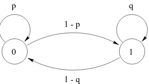
1g

defines a discrete time Markov chain with two states. One of the states denoted by 0 is regarded as success, and the other denoted by 1 as failure. A graphical description of this Markov chain is provided by its state diagram shown in figure 1 and its transition probability matrix is given by

P

=

p

1;

p

1;

q q

0

p q

1. (2)

Since

p

and

q

are probabilities, it follows that

q p

1 - q 1 - p

1 0

Figure 1. Markov interpretation of dependent Bernoulli trials

Let us first consider in some detail the Markov chain. The probability

q

(

p

) is the conditional probability of failure (success) on a software run given that the previous run has failed (succeeded). The unconditional probability of failure on the(

j

+1)-st run is:

Pr

f

Z

j

+1

=1g

=

Pr

f

Z

j

+1

=1

Z

j

=1g+

Pr

f

Z

j

+1

=1

Z

j

=0g =

Pr

f

Z

j

+1

=1j

Z

j

=1g

Pr

f

Z

j

=1g +

Pr

f

Z

j

+1

=1j

Z

j

=0g

Pr

f

Z

j

=0g =

q Pr

f

Z

j

=1g+(1;

p

)

Pr

f

Z

j

=0g =

q Pr

f

Z

j

=1g+(1;

p

)1;

Pr

f

Z

j

=1g]

=(1;

p

)+(

p

+

q

;1)

Pr

f

Z

j

=1g

:

(4)

If

p

+

q

=1the Markov chain describes a sequence of

independent Bernoulli trials. In that case the equation (4) reduces to

Pr

f

Z

j

+1

=1g=1;

p

=

q

, which means that

the failure probability does not depend on the outcome of the previous run. Thus each subsequent run has indepen-dently probabilities

p

and

q

=1;

p

of being a success and

failure. It follows that the number of failures in

n

runs

S

n

is a sum of

n

mutually independent Bernoulli r.v. and has binomial pmf.

If

p

+

q

6=1then the DTMC describes the sequence of

dependent Bernoulli trials and enables us to accommodate possible dependence among successive runs. In this case the outcome of the software run (success or failure) depends on the outcome of the previous run as in equation (4) and the assumptions of binomial distribution do not hold. The pmf of the number of failures in

n

runs

S

n

, given by the sum of

n

dependent random variables, can be derived using the observation that each visit to a given state of DTMC is a possibly delayed recurrent event [12].

When

p

+

q >

1, runs are positively correlated, that

is, if software failure occurs in

j

-th run, there would be an increased chance that another failure will occur in the next run. It is obvious that in this case failures occur in clusters. The boundary case arises when equality in (3) holds, i.e.,

p

+

q

=2(

p

=

q

=1). This means that if the sequence of

software runs starts with failure all successive runs will fail

or if it starts with success all successive runs will succeed, that is, the Markov chain remains forever in its initial state as shown in figure 2.

1 1

0 1

Figure 2. DTMC for the casep=q=1

Next consider the case when successive software runs are negatively correlated

p

+

q <

1. In other words, if

soft-ware failure occurs in

j

-th run, there would be an increased chance that a success will occur in(

j

+1)-st run, that is,

there is a lack of clustering. In the boundary case, when the equality in (3) holds (

p

+

q

=0, i.e.,

p

=

q

=0), the

Markov chain alternates deterministically between the two states, as in figure 3.

1

1

0 1

Figure 3. DTMC for the casep=q=0

The boundary cases are excluded from further analysis since they are somewhat trivial, with no practical interest. We impose the condition0

< p q <

1on transition

proba-bilities, which implies thatj

p

+

q

;1j

<

1. In other words,

DTMC in figure 1 is irreducible and aperiodic [34].

3.2. Software Reliability Model in Continuous Time

The next step in the model construction is to obtain a process in continuous time considering the time that takes software runs to be executed. Therefore we assign a distri-bution function

F

kl

(

t

)to the time spent in a transition from

state

k

to state

l

of the DTMC in figure 1. It seems realistic to assume that the runs execution times are not identically distributed for successful and failed runs. Thus, distribu-tions

F

kl

(

t

) depend only of the type of point at the end

of the interval, that is,

F

00

(

t

) =

F

10

(

t

) =

F

ex

S

(

t

) and

F

01

(

t

) =

F

11

(

t

) =

F

ex

F

(

t

), where

F

ex

S

(

t

)and

F

ex

F

(

t

)

are the distribution functions of the execution times of suc-cessful and failed runs, respectively.

With the addition of distributions

F

kl

(

t

) to the

software runsf

N

(

t

)

t

0gis a superposition of two

de-pendent renewal processes

N

S

(

t

)and

N

F

(

t

)which refer to

the number of times states0(success) and1(failure) of the

DTMC have been visited in(0

t

].

3.3. Software Reliability Growth Model

In additions to assumptions #1 – #3, this section uses the following

Assumptions

A1 Whenever a failure occurs faults are detected and re-moved instantaneously.

A2 At each such event the probabilities of success and fail-ure will change.

A3 Software execution times are identically distributed for successful and failed runs.

A4 Run’s execution time distribution does not change dur-ing the testdur-ing phase.

Assumptions A1, A3, and A4 can easily be relaxed or re-moved as shown in section 3.4.

During the testing phase software is subjected to a se-quence of runs, making no changes if there is no fail-ure. When a failure occurs on any run an attempt will be made to fix the underlying fault which will cause the condi-tional probabilities of success and failure on the next run to change. In other words, the transition probability matrix

P

i

given by

P

i

=

p

i

1;

p

i

1;

q

i

q

i

(5)

defines the values of

p

i

and

q

i

for the testing runs that fol-low the occurrence of the

i

-th failure up to the occurrence of the next(

i

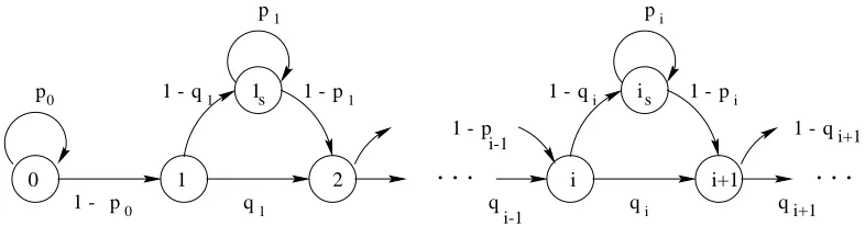
+1)-st failure. Thus, the software reliability

growth model in discrete time can be described with a se-quence of dependent Bernoulli trials with state-dependent probabilities. The underlying stochastic process is a non-homogeneous discrete time Markov chain.

The sequence

S

n

=

Z

1

+

:::

+

Z

n

provides an

alterna-tive description of reliability growth model considered here, that is,f

S

n

gdefines the DTMC presented in figure 4. Both

states

i

and

i

s

represent that failure state has been occupied

i

times. The state

i

represents the first trial for which the accumulated number of failures

S

n

equals

i

, while

i

s

rep-resents all subsequent trials for which

S

n

=

i

, that is, all

subsequent successful runs before the occurrence of next

(

i

+1)-st failure. Without loss of generality we assume that

the first run is successful, that is,0is the initial state.

The model in continuous time is obtained by assigning distribution function

F

ex

S

(

t

)to all transitions to states

i

s

and

F

ex

F

(

t

) to all transitions to states

i

(

i

1) of the

DTMC in figure 4. For the sake of simplicity, we have cho-sen the same execution time distribution regardless of the outcome

F

ex

(

t

) =

F

ex

S

(

t

) =

F

ex

F

(

t

). Thus, the

execu-tion time

T

ex

of each software run has the distribution func-tion

F

ex

(

t

)=

P

f

T

ex

t

g. Considering the situation when

software execution times are not identically distributed for successful and failed runs

F

ex

S

(

t

)6=

F

ex

F

(

t

)is

straightfor-ward and will be discussed later.

In software reliability modeling we are interested in de-riving the distribution of the time between successive fail-ures. This means that only the points of particular type, i.e., failures are of interest. Therefore, it is necessary to con-sider only the distribution of an interval between successive failures and to make use of the standard results of renewal theory. When software reliability growth is considered a usual measure of reliability is conditional reliability. Since the system has experienced

i

failures, conditional reliability is the survivor function associated with(

i

+1)-st failure.

First we derive the distribution of the discrete random variable

X

i

+1 defined as a number of runs between two

successive visits to the failure state of the DTMC, that is, a number of runs between the

i

-th and(

i

+1)-st failure.

Clearly, (see the figure 4) the random variable

X

i

+1 (

i

1)

has the pmf:

Pr

f

X

i

+1

=

k

g=

q

i

if

k

=1

(1;

q

i

)

p

k

;2

i

(1;

p

i

) if

k

2

:

(6)

Next, we derive the distribution of the time to next failure in continuous time which is the interval distribution of the point process

N

F

(

t

)that records the number of failures in

(0

t

]. Let

T

0

i

(

i

=1 2

:::

)be a continuous random variable

representing the occurrence time of

i

-th failure. Define

T

i

+1

as the time elapsed from the

i

-th failure until the occurrence of the(

i

+1)-st failure. It follows that

T

0

i

+1 =

P

i

+1

j

=1

T

j

=

T

0

i

+

T

i

+1 where

T

0 0

=0. We need to derive the distribution

of the interval between successive failures

T

i

+1 =

T

0

i

+1 ;

T

0

i

:

It follows from (6) that the conditional distribution of the time to the(

i

+1)-st failure, given that the system has

experiences

i

failures,

F

i

+1

(

t

)=

P

f

T

i

+1

t

gfor

i

1is

given by:

F

i

+1

(

t

)=

q

i

F

ex

(

t

)+ 1 X

k

=2

(1;

q

i

)

p

k

;2

i

(1;

p

i

)

F

k

ex

(

t

)

(7)

where

F

k

ex

denotes the k-fold convolution of the distribu-tion

F

ex

.

The Laplace-Stieltjes transform (LST) of

F

ex

(

t

)is the

function

F

~

ex

(

s

)defined for

s

0by

~

F

ex

(

s

)= Z

1

0

e

;

st

dF

ex

(

t

)=

E

e

;

st

i 1 2 i_s 1_s

. . .

. . .

p

p p_i

0

1

q₁ q_i

i+1

0

p 1 -

q₁

1 - 1 - p₁ 1 -q_i 1 - p_i

i+1

q q

i-1

1 - p

i-1

0

1 - q_i+1

Figure 4. Nonhomogeneous DTMC model for software reliability growth

The LST of the distribution of the time to next failure

F

i

+1

(

t

)becomes

~

F

i

+1

(

s

)=

q

i

~

F

ex

(

s

)+ 1 X

k

=2

(1;

q

i

)

p

k

;2

i

(1;

p

i

) ~

F

_kex

(

s

)

=

q

i

F

~

ex

(

s

)+(1;

p

i

;

q

i

) ~

F

2

ex

(

s

) 1;

p

i

~

F

ex

(

s

)

:

(8)

The inversion of (8) is in principle straightforward and rea-sonably simple closed form results can be obtained when the run’s execution time distribution

F

ex

(

t

) has rational

LST (such as phase type distributions discussed in [4]). We can develop some general properties of time to next failure without making assumptions about the form of the run’s execution time distribution

F

ex

(

t

). Due to the well

known property of LST the moments can be derived easily by a simple differentiation of (8). Thus, the mean time to failure is

E

T

i

+1

]=;

d

F

~

i

+1

(

s

)

ds

s

=0 =;

2;

p

i

;

q

i

1;

p

i

d

F

~

ex

(

s

)

ds

s

=0 =

2;

p

i

;

q

i

1;

p

i

E

T

ex

] (9)

where

E

T

ex

] is the run’s mean execution time. It can

be shown that, on average, there is growth in reliability

E

T

i

+1

]

> E

T

i

]if and only if

1;

q

i

+1

1;

p

i

+1

>

1;

q

i

1;

p

i

:

If

p

i

+

q

i

=1then successive runs are independent and

(9) becomes

E

T

i

in

+1

]=

E

T

ex

] 1;

p

i

which means that we can rewrite (9) as

E

T

i

+1

]=(2;

p

i

;

q

i

)

E

T

i

in

+1

]

:

If we introduce the notation

i

=

p

i

+

q

i

;1then

E

T

i

+1

]=(1;

i

)

E

T

i

in

+1

]

:

(10)

Next, we derive the expression for the variance

V ar

T

i

+1

] =

2

T

i+1

which is the measure of spread or dis-persion of a distribution. First we derive

E

T

2

i

+1 ]=

d

2 ~

F

i

+1 (

s

)

ds

2

s

=0

and then substitute it together with (9) in

V ar

T

i

+1

]=

E

T

2

i

+1

];(

E

T

i

+1

]) 2

:

It follows that the expression for

V ar

T

i

+1

]in terms of

vari-ance

V ar

T

ex

]and mean

E

T

ex

]of the run’s execution time

is given by

V ar

T

i

+1

]=

2;

p

i

;

q

i

1;

p

i

V ar

T

ex

]

+

(

p

i

+

q

i

)(1;

q

i

) (1;

p

i

)

2

(

E

T

ex

]) 2

:

(11)

Besides the mean and variance, one particularly impor-tant feature of distributions is the coefficient of variation

C

T

i+1, defined by ratio of the standard deviation to the mean

C

T

i+1 =

T

i+1

E

T

i

+1

]

:

(12)

C

T

i+1is a relative measure of the spread of the distribution,

and the idea behind its use is that a deviation of amount

T

i+1 is less important when

E

T

i

+1

] is large than when

E

T

i

+1

]is small. Substituting (9) and (11) into (12) leads

to

C

2

T

i+1 =

1

2;

p

i

;

q

i

C

2

T

in i+1

+

(

p

i

;

q

i

)(

p

i

+

q

i

;1) (2;

p

i

;

q

i

)

2

(13)

where

C

T

in i+1

A very plausible assumption for any software is that the probabilities of failure are much smaller than the probabil-ities of success, that is,

p

i

> q

i

. A program for which this assumption could not be made would be enormously unreli-able, and it is unlikely that its use would be ever attempted. It follows that the sign of the second term in equation (13) will depend only on

i

=

p

i

+

q

i

;1.

The derived equations for the mean time to failure (10) and the coefficient of variation (13) enable us to study the effects of failure correlation on software reliability. When the successive software runs are dependent(

i

6= 0)two

cases can be considered:

1. If0

<

i

<

1 (

p

i

+

q

i

>

1)then successive runs

are positively correlated, that is, the failures occur in clusters. It follows from (10) that the mean time be-tween failures is shorter than it would be if the runs were independent

E

T

i

+1

]

< E

T

i

in

+1

]. Since the

sec-ond term in (13) is positive it follows that

C

2

T

i+1

>

1

1; i

C

2

T

in i+1

> C

2

T

in i+1

. These results imply that in the presence of failure clustering the inter-failure time has smaller mean and greater variability compared to the independent case. In other words, SRGM that assume independence among failures will result in overly op-timistic predictions.

2. If;1

<

i

<

0 (

p

i

+

q

i

<

1)then successive runs

are negatively correlated, that is,

E

T

i

+1

]

> E

T

i

+1

F

].

In this case the second term in (13) is negative and hence

C

2

T

i+1

<

1 1;

i

C

2

T

in i+1

< C

2

T

in i+1

. It follows that assuming a lack of clustering leads to greater mean and smaller variability of the inter-failure times compared to the independent case.

3.4. Model Generalizations

The presented model can be generalized in many ways. We next present some of these generalizations, together with brief comments on the nature of new ideas involved.

First, considering non-identically distributed execution times for successful and failed runs

F

ex

S

(

t

)6=

F

ex

F

(

t

), that

is, replacing assumption A3 with assumption 4 is straight-forward; we assign distribution function

F

ex

S

(

t

)to each

transitions to state

i

s

(successful runs), and

F

ex

F

(

t

)to each

transition to state

i

(failed runs). By making appropriate changes in (7) we get:

F

i

+1

(

t

)=

q

i

F

ex

F

(

t

)

+ 1 X

k

=2

(1;

q

i

)

p

k

;2

i

F

(

k

;1)

ex

S

(

t

)(1;

p

i

)

F

ex

F

(

t

)

(14)

which leads to LST transform:

~

F

i

+1 (

s

)=

q

i

F

~

ex

F

(

s

)+(1;

p

i

;

q

i

) ~

F

ex

F (

s

)

~

F

ex

S (

s

) 1;

p

i

~

F

ex

S (

s

)

:

(15)

Next generalization considers assumption A4, that is, the possible variability of the run’s execution time distribution

F

ex

(

t

). We have assumed that this distribution does not

change during the whole testing phase. This assumption can be violated for reasons such as significant changes in the code due to the fault fixing attempts. In other words, it may be useful to consider the situation when the parameters of the distribution

F

ex

(

t

)change after each failure occurrence

(i.e., after each visit to the failure state). In that case, we need only to substitute

F

ex

(

t

)with

F

ex

i

(

t

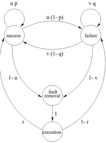
)in equation (7).

One more generalization that can be considered in apply-ing the MRP approach is to choose

m

-state Markov chain to describe the sequence of software runs in discrete space. Thus, it is possible to define DTMC which considers more than one type of failure. We can also add states that will enable us to consider periods of time when the software is idle or non-zero time to remove faults. For example, DTMC presented in figure 5 can be used to describe different test-ing scenarios, such as:

u

=

v

= 1the model reduces to the one considered

previously, that is, instantaneous fault removal which occurs immediately after the failure is observed.

u

= 1 and

v

= 0non-instantaneous fault removal

which occurs immediately after the failure is observed.

u

=1and

v

6=0delayed and non-instantaneous fault

removal following the failure occurrence.

u

6= 1 program can be changed, due to the fault

removal or other modifications, following successful runs as well.

As in the case of SRGM in section 3.3 the transition proba-bilities will change at each visit to fault removal state.

success failure

fault removal

u p

1 1- u

u (1- p)

v q

v (1- q)

1- v

1- r r

execution

Figure 5. DTMC for non-instantaneous and delayed fault removal

4.

APPLICABILITY

TO

VALIDATION

PHASE AND OPERATIONAL PHASE

The presented modeling approach can be used to make reliability estimations of the software based on the results of testing performed in its validation phase. In the case of safety critical software it is common to demand that all known faults are removed. This means that if there is a failure during the testing the fault must be identified and removed. After the testing (debugging) phase the software enters a validation phase in order to show that it has a high reliability prior to actual use. In this phase no changes are made to the software. Usually, the validation testing for safety critical software takes the form of specified number of test cases or specified period of working that must be ex-ecuted failure-free. While of particular interest in the case of safety critical software, the same approach can be applied to any software that, in its current version, has not failed for

n

successive runs.

Let

be the unconditional probability of a failure per run (execution). For the case of independent Bernoulli trials the probabilities that each run will fail

=

q

or succeed1;

=

p

are independent of previous runs. Thus, the probability that

n

independent test runs are conducted without failure is given by

(1;

)

n

=(1;

q

)

n

=

p

n

:

(16)

The largest value of

such that

(1;

)

n

(17)

defines the1;

upper confidence bound on

[11], [34].

Solving (17) for

gives1;

confidence that the failure

probability per execution of a software that reveals no fail-ure in

n

independent runs is below

=1;

1

=n

:

(18)

For the related recent work on a Bayesian estimation ap-proach see [19] and [21].

Now consider a sequence of possibly dependent software runs. During the validation phase the software is not chang-ing, that is,

p

and

q

do not vary. In other words, the sequence of runs can be described by the homogeneous DTMC with transition probability matrix (2). We assume that the DTMC is stationary, that is, each run has the same probability of failure

Pr

f

Z

j

+1

=1g =

Pr

f

Z

j

=1g =

. Then, from

(4) it follows that

=

1;

p

2;

p

;

q:

(19)

The probability that

n

successive runs will succeed is given by:

Pr

f

Z

n

=

:::

=

Z

2

=

Z

1

=0j

Z

0

=1g

=

Pr

f

Z

n

=0j

Z

n

;1

=0g

:::Pr

f

Z

2

=0j

Z

1

=0g

Pr

f

Z

1

=0j

Z

0

=1g

=

p

n

;1

(1;

q

)

:

(20)

Using the notation

=

p

+

q

;1in addition to (19) we

can rewrite (20) in terms of

and

. It follows that in the case of dependent Bernoulli trials(1;

)upper confidence

bound on failure probability per execution

becomes:

=

1;

1

=

(

n

;1)

1;

:

(21)

If failures occur in clusters (0

< <

1) then the confidence

bound on failure probability is approximately 1

=

(1;

)

higher than the bound obtained under the independence as-sumption (18), that is, the result obtained under the assump-tion of independence is overly optimistic.

the expected number of failures

M

F

(

t

) =

E

N

F

(

t

)]

and the expected number of successes

M

S

(

t

) =

E

N

S

(

t

)]in the interval(0

t

];

the probability of success at time

t

, that is, instanta-neous availability;

the limiting probability that the process will be in state

0at time

t

as

t

!1, that is, steady-state availability.

Finally, the Markov renewal modeling approach can be used for modeling fault-tolerant software systems. Per run failure probability and run’s execution time distribution for particular fault-tolerant technique can be derived using a va-riety of existing models (see [30], [10], [20] and references therein). Thus, in addition to the interversion failure corre-lation on a single run considered in related works, our ap-proach enables to account for the correlation among succes-sive failures.

5. SOME SPECIAL CASES AND RELATION

TO EXISTING MODELS

The Markov renewal model described in this paper can be related to existing software reliability models. The model in discrete time is comparable with an input-domain based models which are static and don’t consider the time, while the model in continuous time is comparable with time-domain software reliability growth models. We next examine these relations.

The software reliability model in discrete time presented in this paper can be related to input-domain based models which consider the software input space from which test cases are chosen. For example, the input-domain model presented in [24] defines

i

(0

i

1) as a fault size

un-der operational inputs after the

i

-th change to the program, that is, given that

i

faults have been detected and corrected. Then the probability that there will be

k

0successful runs

before the occurrence of the next(

i

+1)-st failure is given

by

P

i

(

k

j

i

)=(1;

i

)

k

i

:

(22)

It is obvious that (22) is a special case of (6) under the assumption that successive inputs have independent fail-ure probability. In [24]

i

is treated as a random vari-able with a distribution function

G

(

i

), and (22) becomes

P

i

(

k

)= R

(1;

i

)

k

i

dG

(

i

)=

E

(1;

i

)

k

i

]

:

Note that the model in discrete time is also related to the Compound-Poisson software reliability model in [27]. This model is based on the work presented in [28] which approximates the sum of dependent integer-valued random variables

S

n

given by (1) with a compound Poisson process when these random variables are rarely nonzero and given

they are nonzero their conditional distributions are nearly identical.

Now consider the software reliability model in contin-uous time. If

F

~

ex

(

s

)is a rational function of

s

, so too is ~

F

i

+1

(

s

), and the inversion of (8) is in principle

straight-forward. An important special case is when the distri-bution of the run’s execution time is exponential so that

f

ex

(

t

)=

e

;

t

, since it relates the MRP approach to the existing time-domain based software reliability models and some of their basic assumptions, such as the independence of successive runs and the exponential distribution of the inter-failure times. In other words, the simplest special case of the model is under the assumptions that the successive software runs are independent (

p

i

+

q

i

= 1) and the

soft-ware execution time (duration of testing runs) is exponen-tially distributed with rate

. Inverting (8) leads to the pdf of the inter-failure times:

f

i

+1

(

t

)=(1;

p

i

)

e

;(1;

p

i)

t

(23)

that is, the conditional reliability is given by

R

i

+1

(

t

)=1;

F

i

+1

(

t

)=

e

;(1;

p

i)

t

:

(24)

It follows that the inter-failure time is exponentially dis-tributed with rate(1;

p

i

)

if the software testing is

consid-ered as a sequence of independent runs with an exponential distribution of the execution times. Note that, the coefficient of variation of an exponential distribution is1.

The alternative interpretation of this special case can be found in [15]. Under the assumption that inputs arrive at software system according to a Poisson process with rate

which is interpreted as intensity of testing, the probability that the software encounters no failures in a time interval

(0

t

]is given by:

1;

F

(

t

)= 1 X

j

=0

e

;

t

(

t

)

j

j

!

M

;

M

M

j

(25)

where

M

is the size of the input data space, i.e., the number of data items which can be used as input to the software and

M

is the total number of these input data which may cause software failure. The first term inside the summation sign denotes the probability that

j

inputs are received in time

t

, and the second term denotes that none of

j

inputs lead to a failure of software. It is easy to verify that (25), when simplified, leads to

1;

F

(

t

)=

e

;

M

M

t

:

(26)

It means that the time to first failure has an exponential distribution with failure rate = (

M

=M

)

. Note that

M

=M

is just the probability of failure on a test run. The conditional reliability, that is, the survivor function of the time between(

i

;1)-st and

i

-th failure

T

i

becomes

1;

F

i

(

t

)=

P

f

T

i

> t

g=

e

;

i

t

:

Even though the motivations are different and the pa-rameters have different interpretations, mathematically the model derived in [15] is a special case of the software re-liability model based on MRP under the assumptions that successive software runs are independent and the software execution times are exponentially distributed with rate

. In [15] it is shown that the Jelinski – Moranda model [14] can be obtained by introducing

i

=

M

(

N

;

i

+1) =

(

N

;

i

+1)and treatingand

N

as unknown

parame-ters. Then by adopting a Bayesian point of view two other models can be derived from the Jelinski – Moranda model [15]:

1. Goel – Okumoto model [7] is obtained by assuming

has a known value and assigning Poisson prior distri-bution for

N

;

2. Littlewood – Verrall model [17] is obtained by assum-ing

N

has a known value and thathas a prior gamma

distribution.

Some other time-domain SRGM can easily be obtained as special cases under the assumption of independence. For example, Moranda model [22] also assumes independent exponentially distributed times between failures with a fail-ure rate that decreases in geometric progression on the oc-currence of each individual failure

i

=

k

i

;1

, where

k <

1. Due to the space limitations and vast number of

SRGM the analysis of the relation to the existing models will not be pursued any further.

Let us now keep the assumption that the distribution of the run’s execution time is exponential, but assume depen-dence between successive software runs (

p

i

+

q

i

6=1).

In-verting (8) leads to the pdf of the inter-failure time given by:

f

i

+1 (

t

)=

(1;

q

i

)

p

i

(1;

p

i

)

e

;(1;

p

i)

t

+

(

p

i

+

q

i

;1)

p

i

e

;

t

:

(28)

This distribution is a mixture (compound) distribution [34] with pdf of a form

g

(

t

) =

1

g

1 (

t

)+

2

g

2

(

t

), where

1

2

>

0and

1

+

2 =1.

In the case when

p

i

+

q

i

>

1 the inter-failure

distri-bution (28) is hyperexponential, that is, a mixture of two exponential distributions with rates(1;

p

i

)

and

. The

mixing probabilities are given by

1

= (1;

q

i

)

=p

i

and

2

=(

p

i

+

q

i

;1)

=p

i

, respectively. Note that the coefficient

of variation in the case of hyperexponential distribution is greater than1. It is obvious that due to the presence of

fail-ure clustering, the inter-failfail-ure time has smaller mean and greater variability compared to the independent case, even under the assumption of exponentially distributed duration of testing runs.

If the

p

i

+

q

i

<

1then (28) becomes a mixture of an

expo-nential distribution with rate(1;

p

i

)

and hypoexponential

distribution with rates(1;

p

i

)

and

. The mixing

propor-tions are

1

=

q

i

=

(1;

p

i

)and

2

=(1;

p

i

;

q

i

)

=

(1;

p

i

),

respectively. It can be shown that the coefficient of vari-ation in this case is smaller than 1. In other words, the

inter-failure time has greater mean and smaller variability compared to the independent case.

The presented results clearly demonstrate the effects of failure correlation on the software reliability measures. It is obvious that some of the common assumptions made by software reliability models are inadequate and result in op-timistic estimations when failures are indeed clustered.

6. DISCUSSION AND FUTURE WORK

The ultimate goal when developing reliability growth models is the development of good reliability inference and prediction methods which can be applied to software devel-opment. This paper does not deal with inference or predic-tions per se. It is mainly aimed at showing that the classical software reliability theory can be extended in order to con-sider a sequence of possibly dependent software runs, that is, failure correlation. However, there are many research is-sues that we would like to address in near future in order the model to be fully specified and applied in real software development projects for performing estimations and pre-dictions.

Let us consider in some detail the concept of software runs. The operation of software can be broken down into series of runs [23]. Each run performs mapping between a set of input variables and a set of output variables and consumes a certain amount of execution time. The input variable for a program run is any data item that exists ex-ternal to the run and is used by a run. There does not have to be a physical input process. The input variable may sim-ply be located in memory, waiting to be accessed. Even for the software that operates continuously it is still possi-ble and more convenient to divide the operation into runs by subdivision of time associated with some user-oriented tasks [23]. The information associated with software runs can generally be grouped into two categories:

Timing. This includes specific time associated with

each run, such as start time, normal termination time for successful runs, or failure time for failed runs.

Input and Outcome. The descriptive information about

each specific run generally specifies the input for the program, the testing environment, and the outcome that has been obtained (success or failure).

and testing process management purposes [31], [32]. This data, with possibly minor modifications, provide common source for reliability growth modeling, input-domain anal-ysis, and integrated analysis in this paper. The Markov re-newal model takes into consideration all the knowledge that we have about system, that is, the outcomes and execution times of all testing runs, either successful or failed.

The existing time-domain SRGM disregard the success-ful runs between two failures and ignore the information conveyed by them. The consideration of successful runs, that is, non-failure stops of software operation for parame-ters estimation of some of the existing SRGM was presented recently in [2]. In this work it is pointed out that disregard-ing the non-failure stops violates the Maximum Information Principle that suggests to exploit available software reliabil-ity information as much as possible.

In the case of MRP model the time between failures

T

i

+1

is a random variable whose distribution depends on the dis-tribution of the run’s execution time

F

ex

(

t

), and on the

con-ditional probabilities

p

i

and

q

i

. The timing information as-sociated with each run can be obtained quite easily in many computer systems. Therefore, instead of making assump-tions, the specific distribution function of the run’s execu-tion time

F

ex

(

t

)could be determined from measured data.

Consider possible models for the parameter set

f

p

1

q

1

p

2

q

2

:::

gnext. It is mathematically possible to

permit an infinite number of failures, and in this case the parameter set is infinite. By setting

q

i

= 0and

p

i

=1for

i

n

+1the finite failure model is obtained as a special

case.

For the model to be fully specified it is necessary to consider the way the parameters change as a result of the fault removal attempts. In this regard, there are two possi-ble approaches. One approach of modeling the parameter setf

p

i

q

i

gis to relate them to the number of test runs or

to the number of faults in a systematic way by assuming various deterministic functional relationships. That is, the free parameters are simply seen as unknown constants to be estimated by the sample data. The alternate approach is to treat the parametersf

p

i

q

i

gas random variables

them-selves in order to consider the uncertainty about the effect of fault removal [18], [17]. Thus, even if the fault removal is successful, there will be uncertainty about the size of the fault removed, and so uncertainty about the magnitude of reliability improvement. This approach results in a doubly stochastic model: one model for set of parameters and the other for the times between failures conditional on the pa-rameters.

We next present the brief review of SRGM discussed in previous section in order to demonstrate the differences that arise from the additional assumptions considering the way the modeling parameters change as a result of the fault re-moval attempts.

Jelinski – Moranda model [14], Moranda model [22], and Littlewood – Verrall model [17] are examples of TBF models and all have the common assumption that the inter-failure times are independent exponentially distributed ran-dom variables

f

i

+1

(

t

)=

i

e

;

i

t

. They differ in assump-tions about the way failure intensity

i

changes as a result of fault removal attempts.

Jelinski – Moranda model assumes that the initial num-ber of faults

N

is unknown fixed constant, faults are in-stantly and perfectly corrected without introducing any new faults, and all faults that still remain are equally likely to occur. As a consequence, failure intensity is proportional to the residual number of faults

i

=(

N

;

i

+1), that is, all

faults have the same size. Moranda model assumes that the initial number of faults is infinite and that the faults detected and removed early in the software testing decrease failure intensity more rapidly from those detected later on. Thus the failure intensity decreases in a geometric progression on the occurrence of each individual failure

i

=

k

i

;1

(

k <

1).

Littlewood – Verrall model is a doubly stochastic model which treats the failure intensity

i

as a random variable with gamma distribution. This reflects the likelihood, but not a guarantee, that a fault removal will improve reliability and if an improvement takes place it is of uncertain magni-tude.

Goel – Okumoto model [7] treats the initial number of faults in software system

N

as a Poisson random variable which results in non-homogeneous Poisson process (NHPP) with failure intensity (

t

). However, failure occurrence rate

per fault for this model is constant, that is, all faults have same size. In contrast to the constant fault detection rate of Goel – Okumoto model, many commonly used FC models are obtained by choosing different (

t

)which results in

dif-ferent NHPP that can capture increasing/decreasing failure occurrence rate per fault. The SRGM based on NHPP dif-fer from TBF models in one more aspect, the inter-failure times are not independent and the non-stationarity of the process complicates their distributions. Nevertheless, it can be shown that if NHPP has failure intensity (

t

)then,

given that there are

n

failures in interval0

t

), these

fail-ures are independent and identically distributed with den-sity (

t

)

=

R

t

0

(

u

)

du

[3].

in order to apply the model to real data, the development of more detailed and specific models within this framework, as well as statistical inference procedures for modeling pa-rameters are the subjects of our future research. Some basic issues that should be taken into account when making addi-tional assumptions about the fault removal process and the way that modeling parameters change as a result of fault removal attempts [1], [35] are briefly outlined here:

Size of faults. In general, different software faults do

not affect equally the failure probability. Some faults which are more likely to occur contribute more to the failure probability than other faults.

Imperfect debugging. Often, fault fixing cannot be

seen as a deterministic process, leading with certainty to the removal of the fault. It is possible that an attempt to fix one fault may introduce new faults in code.

Non-instantaneous and delayed fault removal.

Usu-ally, neither the removal of a fault occurs immediately after the failure is observed, nor the time to remove the fault is negligible.

Changing testing strategy. The failure history of a

pro-gram depends on the testing strategy employed, so re-liability models must consider the testing process used. In practice it is important to deal with the case of non-homogeneous testing, that is the model should include the possibility of describing variations of the testing strategy with time.

ACKNOWLEDGMENT

This research was supported in part by the National Sci-ence Foundation under an IUCRC TIE project between Pur-due SERC and CACC-Duke Grant No. EEC-9714965, by Bellcore (now Telcordia), by the Department of Defense Grant No. EEC-9418765, and by the Lord Foundation as a core project in the Center for Advanced Computing and Communication at Duke University.

References

[1] S.Bittanti, P.Bolzern, R.Scattolini, “An introduction to software reliability modeling”, Software

Reliabil-ity Modelling and Identification (S.Bittanti, Ed), 1988,

pp 43 – 66; Lecture Notes in Computer Science, vol 341, Springer – Verlag.

[2] K.Cai, “Censored software-reliability models”, IEEE

Trans. Reliability, vol 46, num 1, 1997 Mar, pp 69 –

75.

[3] D.R.Cox, V. Isham, Point Processes, 1980; Chapman and Hall.

[4] D.R.Cox, H.D.Miller, The Theory of Stochastic

Pro-cesses, 1990; Chapman and Hall.

[5] L.H.Crow, N.D.Singpurwalla, “An empirically devel-oped Fourier series model for describing software fail-ures”, IEEE Trans. on Reliability, vol R-33, num 2, 1984 June, pp 176 – 183.

[6] W.Farr, “Software reliability modeling survey”,

Hand-book of Software Reliability Engineering, (M.R.Lyu, Ed), 1996, pp 71 – 117; McGraw–Hill.

[7] A.L.Goel, K.Okumoto, “Time dependent error-detection rate model for software reliability and other performance measures”, IEEE Trans.

Reliabil-ity, vol R-28, 1979, pp 206 – 211.

[8] S.Gokhale, P.N.Marinos, K.S.Trivedi, M.R.Lyu, “Ef-fect of repair policies on software reliability”, Proc.

Computer Assurance (COMPASS’97), 1997, pp 105–

116.

[9] S.Gokhale, M.Lyu, K.Trivedi, “Software reliability analysis incorporating fault detection and debugging activities”, Proc. 9th IEEE Int’l Symp. Software

Reli-ability Engineering, 1998, pp 202–211.

[10] K.Goˇseva – Popstojanova, A.Grnarov, “Hierarchical Decomposition for Estimating Reliability of Fault-Tolerant Software in Mission-Critical Systems”, Proc.

IASTED Int’l Conf. Software Engineering, 1997,

pp 141–146.

[11] D.Hamlet, “Are we testing for true reliability?”, IEEE

Software, 1992 July, pp 21 – 27.

[12] J.J.Hunter, Mathematical Techniques of Applied

Prob-ability, Volume 2, Discrete Time Models: Techniques and Applications, 1983; Academic Press.

[13] Handbook of Software Reliability Engineering,

(M.R.Lyu Ed), 1996; McGraw–Hill.

[14] Z.Jelinski, P.B.Moranda, “Software reliability re-search”, Statistical Computer Performance

Evalua-tion, (W.Freiberger, Ed), 1972, pp 485 – 502;

Aca-demic Press.

[15] N.Langberg, N.D.Singpurwalla, “A unification of some software reliability models”, SIAM J. Sci. Stat.

Comput., vol 6, num 3, 1985 July, pp 781 – 790.

[16] J.Laprie, K.Kanoun, “Software reliability and system reliability”, Handbook of Software Reliability

Engi-neering, (M.R.Lyu, Ed), 1996, pp 27 – 69; McGraw–

[17] B.Littlewood, J.L.Verrall, “A Bayesian reliability growth model for computer software”, Proc. IEEE

Symp. Computer Software Reliability, 1973, pp. 70 –

77.

[18] B.Littlewood, “Modeling growth in software relia-bility”, Software Reliability Handbook, (P.Rook Ed), 1990, pp 137 – 153; Elsevier Applied Science.

[19] B.Littlewood, D.Wright, “Some conservative stopping rules for the operational testing of safety-critical soft-ware”, IEEE Trans. Software Engineering, vol 23, num 11, 1997 Nov, pp 673 – 683.

[20] D.F.McAllister, M.A.Vouk, “Fault-Tolerant Software Reliability Engineering”, Handbook of Software

Re-liability Engineering, (M.R.Lyu, Ed), 1996, pp 567–

614; McGraw–Hill.

[21] K.W.Miller, L.J.Morell, R.E.Noonan, S.K.Park, D.M.Nicol, B.W.Murrill, J.M.Voas, “Estimating the probability of failure when testing reveals no failures”, IEEE Trans. Software Engineering, vol 18, num 1, 1992 Jan, pp 33 – 43.

[22] P.B. Moranda, “Prediction of software reliability dur-ing debuggdur-ing”, Proc. Annual Reliability and

Main-tainability Symposium, 1975, pp 327 – 332.

[23] J.D.Musa, A.Iannino, K.Okumoto, Software

Relia-bility: Measurement, Prediction, Application, 1987;

McGrow–Hill.

[24] C.V.Ramamoorthy, F.B. Bastani, “Modeling of the software reliability growth process”, Proc.

COMP-SAC, 1980, pp 161 – 169.

[25] C.V.Ramamoorthy, F.B. Bastani, “Software reliabil-ity – status and perspectives”, IEEE Trans. Software

Engineering, vol SE-8, num 4, 1982 July, pp 354 –

371.

[26] S.M.Ross, Applied Probability Models with

Optimiza-tion ApplicaOptimiza-tions, 1970; Holden – Day.

[27] M.Sahinoglu, “Compound-Poisson software relia-bility model”, IEEE Trans. Software Engineering, vol SE-18, num 7, 1992 July, pp 624 – 630.

[28] R.F.Serfozo, “Compound Poisson approximations for sums of random variables”, Annals of Probability, vol 14, num 4, 1986, pp 1391 – 1398.

[29] Software Reliability Modelling and Identification, (S. Bittanti Ed), 1988; Lecture Notes in Computer Sci-ence, vol 341, Springer – Verlag.

[30] A.T.Tai, J.F.Meyer, A.Aviˇzienis, “Performability En-hancement of Fault-Tolerant Software”, IEEE Trans.

on Reliability, vol 42, num 2, 1993 June, pp 227–237.

[31] J.Tian, “Integrating time domain and input domain analyses of software reliability using tree-based mod-els” IEEE Trans. Software Engineering, vol 21, num 12, 1995 Dec, pp 945 – 958.

[32] J.Tian, J.Palma, “Data partition based reliability mod-eling” Proc. 7th IEEE Int’l Symp. Software Reliability

Engineering, 1996, pp 354 – 363.

[33] L.A.Tomek, J.K.Muppala, K.S.Trivedi, “Modeling correlation in software recovery blocks” IEEE Trans.

Software Engineering, vol 19, num 11, 1993 Nov,

pp 1071 – 1086.

[34] K.S.Trivedi, Probability and Statistics with

Relia-bility, Queuing and Computer Science Applications,

1982; Prentice – Hall.

[35] M.Xie, Software Reliability Modelling, 1991; World Scientific Publishing Company.

AUTHORS

Dr. Katerina Goˇseva – Popstojanova; Dep’t of Electrical & Computer Eng’g; Duke University; Durham, North Car-olina 27708–0291 USA.

Internet (e-mail): katerina@ee.duke.edu

Katerina Goˇseva - Popstojanova received BS (1980), MS (1985) and PhD (1995) degrees in Computer Science from the Faculty of Electrical Engineering, University “Sv. Kiril i Metodij”, Skopje, Macedonia. Since 1997 she has been working as an Assistant Professor in the Department of Computer Science at Faculty of Electrical Engineering, University “Sv. Kiril i Metodij”. Currently she is a visiting scholar in the Department of Electrical and Computer Engineering at Duke University. Her research interests include software reliability, fault–tolerant computing, and dependability, performance and performability modeling; she has published numerous articles on these topics. She is a Member of IEEE.

Dr. Kishor S. Trivedi; Dep’t of Electrical & Computer Eng’g; Duke University; Durham, North Carolina 27708– 0291 USA.

Internet (e-mail): kst@ee.duke.edu

Kishor S. Trivedi received the B.Tech. degree from the Indian Institute of Technology (Bombay), and M.S. and Ph.D. degrees in computer science from the University of Illinois, Urbana-Champaign. He is the author of a well known text entitled, Probability and Statistics with

by Prentice-Hall. He has recently published two book en-titled, Performance and Reliability Analysis of Computer

Systems, published by Kluwer Academic Publishers and Queueing Networks and Markov Chains, John Wiley. His