Development of a Novel Residual Formulation of CTF and Application of Parameter Estimation Techniques.

(1)

Abstract

PORTER, NATHAN WAYNE. Development of a Novel Residual Formulation of CTF and Application of Parameter Estimation Techniques. (Under the direction of Maria Avramova).

In modern science, computational modeling and simulation are often used in place of physical experiments. This is especially true in the nuclear power industry, where experiments are prohibitively expensive—or impossible—due to their extreme scales, high temperatures, high pressures, and radiation. Though the advent of the contemporary computer has enabled the design, testing, and construction of hundreds of nuclear reactors throughout the world, most simulation codes currently used in the industry were developed in the 1980’s.

One such code, COolant Boiling in Rod Arrays–Three Field (COBRA-TF), was developed in the 1980’s to model the thermal hydraulic response of water in nuclear reactor cores. The code used in this work, CTF, is a version of COBRA-TF which is currently developed at North Carolina State University. CTF and other “legacy codes” were designed to utilize very limited computational resources, and therefore required many simplifications. Today’s computers have vastly improved memory and speed, and as such, these simplifications are no longer necessary. Though various versions of COBRA-TF have been used extensively throughout academia and industry, its original simplifications are still present in CTF.

A novel residual-based version of CTF, which enables the removal of these simplifications, is developed in this work. The code, called CTF-Residual (CTF-R), allows flexibility in the implicitness, discretization, solution algorithm, physical modeling choices, and numerical solver used to solve the fluid conservation equations. This is an improvement over the current version of CTF, which allows very little flexibility in any of these areas. In addition, CTF-R is designed with modern coding practices—software quality assurance, verification, and validation—in mind.

Currently, CTF-R is capable of modeling single phase flow with wall friction, heat transfer, lateral transfer, and nuclear fuel rods. Verification tests are used to prove that the first order numerical scheme is implemented correctly. Each model in the code is provided with a series of defect tests to ensure that it is accurate and error-free. Some models also include validation tests which compare predicted results to experimental data. Finally, regression tests are incorporated into the code repository to ensure that future changes do not break current capabilities. CTF-R includes four empirical models: wall friction, heat transfer from the nuclear fuel rods to the fluid, thermal conductivity of uranium dioxide, and thermal conductivity of zirconium. A particular correlation is chosen for each of these models, and its origin, assumptions, and an extensive set of experimental data are discussed. Each of the four correlations is calibrated to the experimental data and the resulting parameter uncertainties are included with the code distribution.

(2)

(3)

Development of a Novel Residual Formulation of CTF and Application of Parameter Estimation Techniques

by

Nathan Wayne Porter

A dissertation submitted to the Graduate Faculty of North Carolina State University

in partial fulfillment of the requirements for the Degree of

Doctor of Philosophy

Nuclear Engineering

Raleigh, North Carolina

2018

APPROVED BY:

Vincent Mousseau External Member

Ralph Smith

Kostadin Ivanov Jia (Jason) Hou

(4)

Biography

Nathan graduated summa cumme laude from Oregon State University in 2013 with a Bachelor of Science in nuclear engineering and a music minor. He recieved his master’s degree, also in nuclear engineering, in 2015 from Pennsylvania State University with a minor in computational science. His professional work has focused on development, verification, validation, calibration, and uncertainty quantification of computational tools with emphasis on thermal hydraulic codes for nuclear applications. He currently has five published works in peer-reviewed journals.

• N. W. Porter, V. A. Mousseau, and M. N. Avramova. Quantified validation with uncertainty analysis for turbulent single phase friction models. Nuclear Technology, 2018. Under review.

• K. Maupin, N. W. Porter, and L. Swiler. Validation metrics for deterministic and proba-bilistic data. ASME Journal of Verification, Validation and Uncertainty Quantification, 2018. Accepted for publication.

• N. W. Porter and M. N. Avramova. Validation of CTF pressure drop and void predictions for the NUPEC BWR database. Nuclear Engineering and Design, 337:291–299, July 2018.

https://doi.org/10.1016/j.nucengdes.2018.07.018.

• A. Toptan, N. W. Porter, R. Salko, and M. N. Avramova. Implementation and assessment of wall friction models for LWR core analysis. Annals of Nuclear Engineering, 115(2018):565– 572, February 2018. https://doi.org/10.1016/j.anucene.2018.02.022.

(5)

Acknowledgements

I would like to express my gratitude to Professor Maria Avramova for her continuous support and guidance throughout my studies. In addition, to my mentor at Sandia National Laboratories, Vince Mousseau, for his commitment to my educational development and his willingness to share his insights with me. Also thanks to Ralph Smith and his ex-student, Katie Schmidt, for their help with Bayesian Calibration. I would also like to thank some of my fellow Graduate Students, without their collaboration I would have certainly been lost: Taylor Blyth, Alexander Bennet, and especially Aysenur Toptan. Finally, I would like to thank my friend, Arielle Schoblom, for her proofreading services for this thesis and countless other works.

(6)

List of Tables

Table 2.1 Thermal resistance equations . . . 11

Table 4.1 Boundary conditions and geometry of CTF-R defect tests . . . 39

Table 4.2 Problem Parameters for Isokinetic Advection . . . 47

Table 4.3 Summary of observed orders of accuracy . . . 53

Table 4.4 Summary of rRMSs for separate effects friction validation . . . 57

Table 4.5 CTF-R regression tests . . . 58

Table 5.1 Data sources for single-phase wall friction . . . 66

Table 5.2 Friction factor marginal parameter distributions . . . 69

Table 5.3 Estimated parameter values for mixed-effects friction model . . . 72

Table 5.4 Data sources for the heat transfer correlation . . . 76

Table 5.5 Heat transfer parameter results . . . 78

Table 5.6 Estimated parameter values for mixed-effects heat transfer model . . . 79

Table 5.7 Data sources for the thermal conductivity of fuel . . . 82

Table 5.8 Fuel thermal conductivity marginal parameter distributions . . . 84

Table 5.9 Estimated parameter values for mixed-effects fuel thermal conductivity model 87 Table 5.10 Cladding thermal conductivity marginal distributions . . . 89

Table A.1 Calculation of neglected terms in enthalpy equation . . . 111

Table C.1 Tight bounds on moments of Wilks’ Formula . . . 139

(9)

List of Figures

Figure 2.1 Cross sections of traditional control volumes in CTF . . . 9

Figure 2.2 Example of CTF solid mesh . . . 10

Figure 2.3 Thermal resistance analogy . . . 10

Figure 3.1 General process for establishing code credibility . . . 17

Figure 3.2 UQ and parameter estimation . . . 22

Figure 4.1 CTF-R staggered mesh . . . 33

Figure 4.2 Constant friction factor defect test results . . . 40

Figure 4.3 Friction factor correlation defect test results . . . 41

Figure 4.4 Conduction equation defect test results . . . 42

Figure 4.5 Constant heat rate defect test results . . . 43

Figure 4.6 Cosine heat rate enthalpy defect tests . . . 44

Figure 4.7 Lateral momentum defect tests with different areas . . . 45

Figure 4.8 Lateral momentum defect tests with equal areas . . . 46

Figure 4.9 Square wave advection results . . . 50

Figure 4.10 Square wave temporal convergence study . . . 50

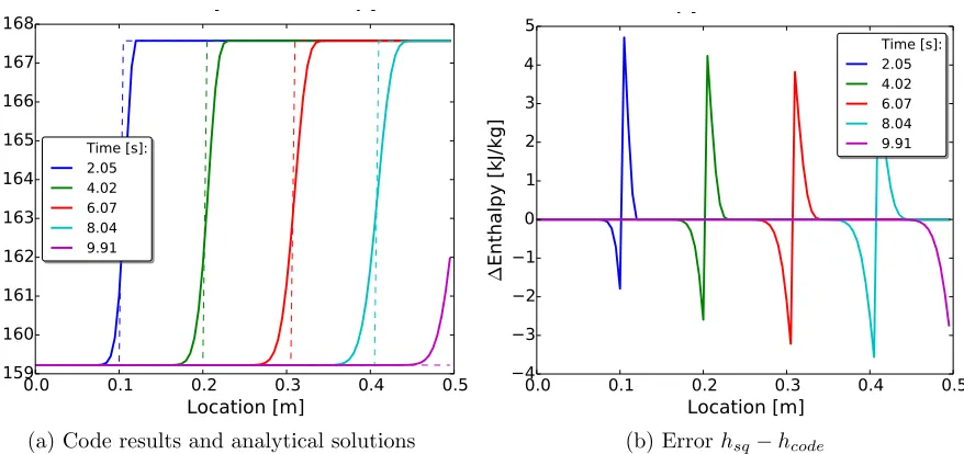
Figure 4.11 Hyperbolic tangent wave advection results . . . 51

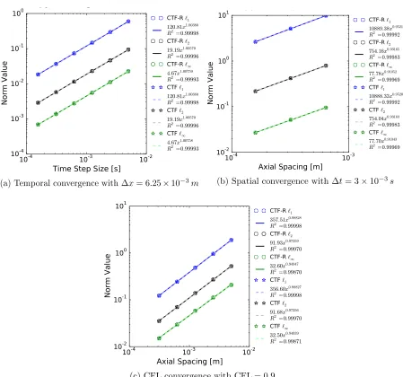
Figure 4.12 Hyperbolic tangent wave convergence studies . . . 52

Figure 4.13 Cosine wave advection results . . . 53

Figure 4.14 Cosine wave convergence studies . . . 54

Figure 4.15 Geometry of friction validation experiments . . . 55

Figure 4.16 Nikuradse pressure drop validation results . . . 56

Figure 4.17 Furuichi pressure drop validation results . . . 56

Figure 4.18 Run times for cosine verification simulations . . . 60

Figure 5.1 Sigmoid function . . . 64

Figure 5.2 Friction factor experimental data . . . 67

Figure 5.3 Friction factor residuals for untransformed data . . . 68

Figure 5.4 Friction factor residuals for transformed data . . . 68

Figure 5.5 Friction factor results . . . 70

Figure 5.6 Friction factor mixed-effects residuals . . . 71

Figure 5.7 Friction factor residual box plots . . . 73

Figure 5.8 Example of mixed-effects results for the friction factor . . . 73

Figure 5.9 Heat transfer experimental data . . . 75

Figure 5.10 Heat transfer residuals for untransformed data . . . 77

Figure 5.11 Heat transfer residuals for transformed data . . . 77

Figure 5.12 Heat transfer marginal parameter distributions . . . 78

Figure 5.13 Heat transfer mixed-effects residuals . . . 80

Figure 5.14 Heat transfer residual box plots . . . 81

Figure 5.15 Fuel thermal conductivity experimental data . . . 83

Figure 5.16 Fuel thermal conductivity residuals . . . 85

(10)

Figure 5.18 Fuel thermal conductivity mixed-effects residuals . . . 88

Figure 5.19 Fuel thermal conductivity residual box plots . . . 89

Figure 5.20 Cladding thermal conductivity experimental data . . . 90

Figure 5.21 Residuals for cladding thermal conductivity model . . . 91

Figure 5.22 Cladding thermal conductivity parameter results . . . 91

Figure B.1 The CTF flow regime map . . . 117

Figure B.2 Diagram of the CTF interfacial mass transfer model . . . 123

Figure B.3 Spatial averaging of the interfacial transfer model . . . 124

Figure C.1 Sample size for Wilks’ Formula . . . 136

Figure C.2 Tight bounds on moments of Wilk’s Formula . . . 140

Figure C.3 Parent distributions for Wilks’ Formula verification . . . 141

(11)

List of Symbols

Greek Letters

α Void fraction [ ]

˙

Γ000 Inter-phase mass transfer [kg/m3·s]

δ Film thickness [f t]

Absolute roughness [m]

ε Observational error

η Fraction of evaporation apportioned to the droplet field [ ]

θ Parameter vector [ ]

µ Dynamic viscosity [P a·s]

ν Kinematic viscosity [m2/s]

π Posterior parameter density [ ]

πo Prior parameter density [ ]

ρ Density [kg/m3]

σ Surface tension [lbf /f t]

τ Shear stress [P a]

˙

Υ000 Inter-field mass transfer [kg/m3·s]

Nondimensional Numbers

f Darcy Friction Factor = 8τw/ρu2

Gr Grashof =gβ∆T D3/ν2 J a Jakob =ρ(hl−hf)/ρvhf g

N u Nusselt =hL/k

P e Peclet =ReP r=cpρvL/k

P r Prandtl =Cpµ/k

Re Reynolds =ρvL/µ

W e Weber =ρu2_D

p/σ

Roman Letters

A Area [m2_]

cp Specific heat [kJ/K]

D Diameter [m]

G Mass Flux [lbm/f t2·s]

h Enthalpy [kJ/kg]

(12)

J Jacobian matrix

k Thermal conductivity [W/m·K]

L Characteristic length [m]

N Number of particles or samples [ ]

P Pressure [P a]

Q Power [btu/s]

q00 Heat flux [W/m2]

q000 Volumetric energy generation [kJ/m3·s]

R Thermal resistance [K/W]

r Radius [m]

˙

s000 Volumetric source term units vary

T Temperature [K]

t Time [s]

u Axial velocity [m/s]

~

u Axial velocity vector [m/s]

V Volume [m3]

w Lateral velocity [m/s]

~

w Lateral velocity vector [m/s]

x Axial position [m]

Subscripts ann Annular

b Bubble

c Cold or cladding

c Critical

cond Conduction

conv Convection

ct Constant

d Droplet

e Entrained droplet

f Fuel

f g Relative between saturated gas and saturated liquid

g Gas or gap

hw Hot wall

(13)

in Inlet

l Liquid/fluid

lb Large bubble

n Non-condensible gas

nb Nucleate boiling

o Outside

out Outlet

p Particle

s Saturated or surface

sb Small bubble

scl Subcooled liquid

scv Subcooled vapor

shl Superheated liquid

shv Superheated vapor

v Gas/vapor

ve Relative between the vapor and entrained droplets

vl Relative between the vapor and liquid

w Wall

wp Wetted perimeter

(14)

CHAPTER

1 INTRODUCTION

The primary responsibility of all Nuclear Power Plant (NPP) engineers, operators, and regulators is to ensure that the public is safe during both normal operating conditions and postulated accidents. In order to do this, these entities must understand the physical phenomena which govern the response of a reactor. The most obvious way to understand reactor responses is through direct experimentation, but in the nuclear industry, this can be inherently dangerous and prohibitively expensive due to the presence of high temperatures, high pressures, and radiation. Therefore, computational tools are often used to supplement experimental data.

In order to be an acceptable supplement, computational models must be accurate representa-tions of reality. “Legacy codes,” which were written in the 1970’s and 1980’s, were significantly impacted by the computational limitations at the time. For example, the amount of memory available was very small, therefore large matrices couldn’t be stored. This restricted most codes to explicit numerical methods, since Jacobian matrices couldn’t be stored in memory. As another example, early computers were very slow, which often limited the complexity or number of models that could be included in the code. Due to these types of limitations, a large number of simplifications were applied to legacy codes that were not always applicable and could introduce a significant amount of uncertainty.

(15)

This allowed the general trend of reactor behavior to be estimated with the belief that the real reactor would be safer than the simulation. Conservative methods have been used in the nuclear industry for decades, but as computers and knowledge have improved, it has become possible to estimate reactor behavior more accurately.

In 1988, the U.S. Nuclear Regulatory Commission (NRC) changed 10 CFR §50.46, which governs the licensing of new reactors, to allow licensing decisions based on Best Estimate Plus Uncertainty (BEPU) analyses [3]. Instead of calculating conservative estimates, BEPU methods attempt to accurately predict the actual response of a system with its associated uncertainties. This eliminates much of the safety margin fundamental to traditional conservative analyses, enabling efficient operation of NPPs.

In order to apply a BEPU method, it is necessary to understand, document, and quantify all sources of uncertainty in a code. The total uncertainty can be comprised of many different parts, including coding mistakes, input or output errors, numerical discretization errors, numerical convergence errors, statistical errors, model form errors, and parameter uncertainties.

Legacy codes were never intended to utilize BEPU methods, and using them presents a variety of unique challenges. The codes often lack proper documentation and it is therefore difficult to decipher the underlying physics or numerical methods. Individual empirical relations are often chosen to be conservative, and therefore must be changed for the application of BEPU methods. Moreover, the individual empirical correlations often were not designed to have inherent uncertainty information.

The motivation of this work is to transition a legacy thermal hydraulic subchannel code, Coolant Boiling in Rod Arrays–Three Field (COBRA-TF), towards more modern BEPU methods. This goal will be achieved via two separate, albeit related, tasks. The first will be to develop a novel residual formulation of the code that will provide more flexibility and be easier to use. Through the development of a new code, the numerical assumptions and inherent conservativism of the legacy version can be avoided. The second task will be to apply modern parameter estimation techniques to achieve BEPU results that are based solely on experimental data. This will supplement the existing coded models with uncertainty information which can be applied in future BEPU analyses.

(16)

CHAPTER

2 THERMAL HYDRAULIC MODELING

Thermal Hydraulic (TH) codes are generally divided into three categories: subchannel analysis, system analysis, and Computational Fluid Dynamics (CFD). There is significant overlap in the methods and theory of these categories, but they are intended for specific purposes.

System analysis software is usually used to analyze an entire plant, including pumps, heat exchangers, valves, etc. Four widely used examples of system codes are Reactor Excursion and Leak Analysis Program (RELAP5-3D©) [5], Methods for Estimation of Leakages and Consequences of Releases (MELCOR) [47], The Code for Analysis of Thermal Hydraulics during an Accident of Reactor and safety Evaluation (CATHARE) [40], and The TRAC/RELAP Advanced Computational Engine (TRACE) [4]. The core models are generally very simple and are used to determine the heat source for the balance of plant. As such, it is often necessary to provide a more detailed analysis of the in-core behavior.

(17)

CFD codes are designed to analyze meshes that are significantly finer than those in system or subchannel codes. CFD codes use turbulence models to replace much of the empirical correlations in other TH codes, and therefore present a higher-fidelity representation of reality. CFD codes can generally only accurately predict the behavior for single-phase flows, though current research focuses on two-phase CFD modeling. Typical CFD codes used in the nuclear industry are Simulating Transport in Arbitrary Regions - Computational Continuum Mechanics (STAR-CCM) [21] and ANSYS Fluent [9]. These codes are generally used to study very specific

and small problems, or when computational cost is not an issue.

This work will focus on COBRA-TF, which was initially developed in the early 1980’s at Pa-cific Northwest National Laboratory (PNNL) to model Loss of Coolant Accidents (LOCAs) [161]. Over time, the code was transferred to many different institutions and a variety of code versions exist throughout academia and industry today. One version, re-branded as CTF, is currently developed and maintained by the Reactor Dynamics and Fuel Modeling Group (RDFMG) at North Carolina State University (NCSU) [13]. CTF was incorporated into The Consortium for Advanced Simulation of LWRs (CASL), which lead to rapid improvements in the code’s capabilities, parallelization, performance, validation, and quality assurance.

First, the CTF conservation equations are introduced in Section 2.1. Then in Section 2.2, the solid energy conservation equation, which is used as a simplified fuel model, will be reviewed. Section 2.3 introduces the meshing and discretization methods. Numerical approximations and solution methods are discussed in Section 2.4.

2.1 Fluid Conservation Equations

In order to solve reactor core behavior during normal operation and safety situations, it is necessary for TH codes to solve the conservation equations for fluids in the reactor. The codes generally solve the equations using a multicomponent fluid approach. Each fluid is assigned its own set of conservation equations, and transfer between the fluids is approximated using mostly empirical models. For the simulation of Light Water Reactors (LWRs), the fluids modeled in the reactor can include liquid water, steam, water droplets, and non-condensible gases.

If conservation equations for all four fluids are modeled completely, there would be a set of twenty equations to solve simultaneously: one mass, three momentum, and one energy equation for each fluid. Since this is generally not realistic, a number of approximations are used to refine the selected equations to a smaller set that still represent reality. The following list explains the particular assumptions used in CTF.

(18)

overwhelms flows in the other directions. As such, subchannel codes generally solve two momentum equations: one for “axial flow” and one for “lateral flow.” Because of this assumption, they cannot accurately model reactor designs with horizontal flow, such as Canada Deuterium Uranium (CANDU) reactors. CTF is generally run with this assumption, though a full three-dimensional implementation is also available.

• The non-condensible gas and steam are in thermal and mechanical equilibrium, and therefore share a common energy and momentum equation.

• The liquid and droplet phases are in thermal equilibrium, and therefore share an energy equation. This assumption is justified by observing that the droplets are constantly entraining from and depositing to the continuous liquid field, and therefore have little time to change temperature.

With these assumptions, the full set of conservation equations is narrowed to twelve: four mass, three axial momentum, three lateral momentum, and two energy. Further assumptions are applied to the conservation equations to introduce empirical relations and to neglect terms that will be small for LWR applications.

• All phases are characterized by a single pressure.

• The vapor and non-condensible components of the gas field obey Dalton’s Law, and therefore occupy the same volume.

• The viscous terms in the momentum and energy equation are neglected since inertial forces are much larger for the problems of interest.

• Empirical correlations are incorporated to account for interfacial transfer, turbulence (frictional forces and heat transfer from the wall), pressure loss coefficients, and other

phenomena.

• Axial pressure drops are relatively small, and therefore the pressure gradient term in the conservation of energy equation is neglected (see Section A.1).

• The droplet field does not contact the wall, and therefore there are no frictional forces on that phase.

• The only body force is that of gravity.

• Axial flow effects are much larger than conduction in the fluid, and it is therefore neglected. • Energy deposited directly in the fluid is assumed to be a percentage of the total energy generated in the reactor. Most of this energy deposition is from interactions of gamma rays with the fluid in the reactor, so it is called gamma heating.

(19)

Manual [13]. The liquid, vapor, entrained droplet, and non-condensible gas mass conservation equations are given in Equations 2.1-2.4, respectively.

∂αlρl

∂t +∇ ·(αlρlu~l) =−(1−η) ˙Γ

000₋ _˙

Υ000+ ˙s000_m,l (2.1) ∂αgρv

∂t +∇ ·(αgρv~ug) = ˙Γ 000

+ ˙s000_m,v (2.2)

∂αeρl

∂t +∇ ·(αeρl~ue) =−ηΓ˙

000_{+ ˙}_Υ000_{+ ˙}_s

m,e (2.3)

∂αgρn

∂t +∇ ·(αgρn~ug) = ˙s 000

m,n (2.4)

The liquid, vapor, entrained droplet, and non-condensible gas are indicated respectively by the subscripts l, v, e, and n. The combined vapor and non-condensible field is indicated by the subscriptg. The first two terms in each mass conservation equation are the temporal and advective term in the Lagrangian derivative of mass for the given field. The mass inter-phase transfer, ˙Γ000, is due to the phase change of water between liquid and vapor. It is defined positive for evaporation. The evaporation of vapor is apportioned to the droplet and liquid phases according to the factor, η, which is between zero and one (η≤1). The inter-field transfer, ˙Υ000, is between the continuous liquid and entrained droplet fields, which accounts for entrainment and de-entrainment of liquid drops. It is defined positive for droplet entrainment. The external source, ˙sm,k, includes turbulent mixing, void drift, and lateral transfer.

Thermodynamic equilibrium between the continuous liquid and entrained droplet phases allows them to be described by a single density,ρl. The non-condensible gas and vapor fields

share a single velocity, ug, since the two phases are in mechanical equilibrium. The two gas

components also occupy the same volume according to Dalton’s law, and therefore share a single volume fraction,αg.

The liquid and gas fields are each described by a conservation of energy equation.

∂(αl+αe)ρlhl

∂t +∇ ·(αlρlhl~ul) +∇ ·(αeρlhl~ue) =−Γ˙000h0_l+q_i,l000−q_n,l000 +q_w,l000 + (αl+αe)

∂P ∂t + ˙s

000

h,l (2.5)

∂αgρghg

∂t +∇ ·(αgρghg~ug)

= ˙Γ000h0_v+q_i,v000 +q000_n,l+q000_w,g+αg

∂P ∂t + ˙s

000

h,g (2.6)

Note that the energy conservation equation is formulated using specific enthalpy, h, rather than energy. The derivation of the enthalpy conservation equation is in Section A.1. The void fractions are related viaαl+αe+αg = 1 and αg=αv+αn. The terms on the left side are the

(20)

The first term on the right side is transfer due to phase change, where h0_k is the enthalpy of the fluid from which the transfer originates. The interfacial transfer rate between thek phase and the saturated interface is q_i,k000,q_w,k000 is the energy transfer rate between solid structures and the kphase, q_n,l000 is the transfer rate of energy between the liquid and non-condensible gas. The pressure work done by thek phase is the term with the pressure derivative. Finally, the external energy source rate for each equation, ˙s000_h,k, accounts for changes in energy due to turbulent mixing, void drift, lateral transfer, and gamma heating.

There is no viscous dissipation or internal generation in the energy equations, since these terms have been neglected. Because the liquid and droplet fields are in thermal equilibrium, they share an energy equation. The non-condensible gas and vapor share an energy equation, and have a common void fraction and velocity. A single pressure, P, is used to define the entire system. For a derivation of the enthalpy equation from the total energy conservation equation, see Section A.1).

There are also momentum equations for the continuous liquid, gas phase, and droplet field.

∂αlρlul

∂t +∇ ·(αlρlul~ul)

=−αl∇P +αlρlg−τw,l000 +τi,gl000 −(1−η) ˙Γ000u0−Υ˙000u0+ ˙s000v,l (2.7)

∂αgρgug

∂t +∇ ·(αgρgug~ug)

=−αg∇P+αgρgg−τw,g000 −τ

000

i,gl−τ

000

i,ge+ ˙Γ

000_u0_{+ ˙}_s000

v,g (2.8)

∂αeρlue

∂t +∇ ·(αeρlue~ue)

=−αe∇P +αeρlg+τi,ge000 −ηΓ˙

000

u0+ ˙Υ000u0+ ˙s000_v,e (2.9)

The left side of these equations is the material derivative of the momentum, and the right side is a variety of surface, boundary, and body forces that act upon them.

(21)

sources of momentum, which for the momentum equation represent turbulent mixing, void drift, and lateral transfer. Axial turbulent stresses are not modeled in CTF, so there is not a term which accounts for this physics.

Finally, there are three lateral momentum equations which account for transfer in the x-y plane. The lateral velocity appears in the other conservation equations in the divergence of the advection the turbulent mixing terms.

∂αlρlwl

∂t +∇ ·(αlρlwl~ul) =−αl

∂P ∂z −τ

000

wx,l+τix,gl000 −(1−η) ˙Γ000w0−Υ˙000w0 (2.10)

∂αgρgwg

∂t +∇ ·(αgρgwg~ug) =−αg

∂P ∂z −τ

000

wx,g−τix,gl000 −τ

000

ix,ge+ ˙Γ000w0 (2.11)

∂αeρlwg

∂t +∇ ·(αeρlwe~ue) =−αe

∂P ∂z +τ

000

ix,ge−ηΓ˙

000

w0+ ˙Υ000w0 (2.12)

All values in the lateral momentum equation have corresponding terms in the axial momentum equations. The lateral direction is defined here as z andw is the lateral velocity component. Once momentum is transferred laterally, it loses its direction. As such, transverse momentum cannot be convected from one gap to another. Such a simplification is only applicable for situations where axial flow is much larger than lateral flow.

2.2 Solid Energy Conservation Equation

CTF has a simple fuel rod model which solves the solid energy equation (or “conduction equation”) for solid components with various geometries. The mass and momentum equations are excluded because thermal expansion is not considered and the solids are stationary. The energy conservation equation can be solved using a finite element or finite volume approach. It has been shown that the finite volume approach is more accurate for models with discontinuous properties [16]. Since nuclear fuel rods have very discontinuous properties due to the cladding and gap regions, a variation of the finite volume approach is used [166]. The control volume form of the conduction equation is shown in Equation 2.13.

d dt

Z

V ρcpT dV = I

A

~

q00_·_dA~ ₊ Z

V q

000_dV₊

I

A

~

q_f00dA~ (2.13)

(22)

accounts for energy conduction in all directions, and the third term is the volumetric generation rate in the solid. The final term accounts for transfer from the solid to the liquid, which will be zero for any control volume that is not at the surface of a solid structure. The area integrals are solved in CTF via a sum over surfaces of each cell, and the volumetric integral of the heat generation is simple since the generation is assumed to be constant for each control volume.

To avoid issues with mass conservation, the expansion or contraction of the fuel is not considered. As such, the density is always evaluated at cold state properties,ρc. The left side of

Equation 2.13 can be simplified since the density does not vary with time and the specific heat is approximated as a linear function.

Z

V ρccp dT

dtdV = I

A

~

q00·dA~ + Z

Vq 000

dV (2.14)

2.3 Meshing and Discretization

A staggered mesh, where velocities are defined at cell faces, is used in CTF. Staggered meshes where first applied to Eulerian codes in the 1960’s [60], and since then have been widely applied in TH codes [42, 60, 127]. CTF uses staggered grids for both the axial and lateral momentum equations (see page 33 for schematic). Each of the axial scalar cells has a cross section which is defined by its flow area and wetted perimeter. These cells are traditionally either channel-centered or rod-centered, both of which are shown in Figure 2.1.

(a) Subchannel-centered (b) Rod-centered

Figure 2.1: Cross sections of traditional control volumes in CTF. Here, the red circles indicate rods and the blue sections are coolant. Subchannel codes generally use control volumes that are defined as the space between four adjacent rods (subchannel-centered), or the space around a rod (rod-centered).

(23)

Fuel Gap Cladding Water Cell Center Cell Edge

Figure 2.2: Example of CTF solid mesh. CTF uses an equally-spaced mesh inside the fuel with cell centers at the outside of the cladding, inside of the cladding, and surface of the fuel.

i−1

i−1_/₂

i _i₊1_/₂ _i_{+ 1}

Ri−3/4 Ri−1/4 Ri+1/4 Ri+3/4 ∆ri−1_/2 ∆ri+1_/2

Ti−1 ki−1

Ti ki

Ti+1 ki+1

Figure 2.3: Thermal resistance analogy. The nomenclature for the four thermal resistances about cell iis established here.

region are equally spaced. It is necessary to interpolate the centerline temperature, since there is not a face at this location. Figure 2.2 is a schematic of the radial fuel meshing.

In CTF, the conduction equation is solved using a thermal resistance analogy. The resistances provide a justifiable method for averaging the thermal conductivity to face values. For example, with a Cartesian mesh, the resistance analogy is equivalent to using a harmonic average of the surrounding control volumes to calculate face thermal conductivities [127]. This method also allows simple treatment of the boundary conditions, gap region, and transfer to the coolant.

A schematic of the thermal resistances about an arbitrary cell iis shown in Figure 2.3 for cylindrical coordinates. For control volume i, the surface heat fluxes in 2.14 can be calculated.

q_i00₋1_/2 =

1 Ri−3_/4+Ri−1_/4

(24)

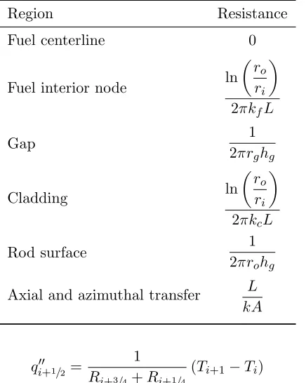
Table 2.1: Thermal resistance equations. All thermal resistances are derived by solving the steady state conduction solution for a particular geometry. This results in relatively simple relations that are easy to implement in a code.

Region Resistance

Fuel centerline 0

Fuel interior node ln

ro

ri

2πkfL

Gap 1

2πrghg

Cladding ln

ro

ri

2πkcL

Rod surface 1

2πrohg

Axial and azimuthal transfer L kA

q_i00₊1_/2 =

1 R_i₊3_/4+Ri+1_/4

(Ti+1−Ti) (2.16)

Here, the resistances and temperatures refer to those in Figure 2.3. The resistances of the corresponding regions are calculated according to a steady state conduction solution for the given fuel cell. Boundary conditions and gap transfer are included as resistances. The equations to calculate each of the thermal resistances are listed in Table 2.1 [161, 162, 166]. The thermal resistances are updated explicitly.

Axial and azimuthal transfer are added as explicit terms in CTF. The axial mesh in the solid region is the same as the fluid region, so each surface solid cell transfers its energy directly to a single fluid cell.

2.4 Numerical Methods

The conservation equations for mass, momentum, and energy can be arranged and solved in a variety of ways. In the most general sense, the discretized form of the equations are arranged in a matrix and solved for the unknown vector of variable updates,δx.

(25)

Here, J is the Jacobian matrix and f(x) is the residual vector. Each row in the Jacobian is related to a specific conservation equation and each column is one of the unknown variables. Most numerical methods are iterative, and convergence is reached when the change between iterations is sufficiently small. In CTF, the full Jacobian matrix is row-reduced to solve for the pressures in each fluid cell.

J0δP =b (2.18)

Here, J0 is the pressure matrix, δP are the pressure updates, and bis the row-reduced right hand side. In this way, all fluid conservation equations are incorporated into a single n×n matrix, where nis the number of computational cells. See [12, Section 3.1] for a description of the pressure matrix construction and solution algorithm.

The fluid conservation equations do not have a general closed-form solution, so it is necessary to find a numerical approximation. The simplifications necessary to find this solution are discussed next.

The first approximation deals with the discretization of the conservation equations in space. Since the continuous form of the equation cannot be solved numerically, one must make an assumption about how the value of all quantities vary throughout a control volume. In CTF, all quantities are assumed to be a constant average value for a specified control volume:

¯ ψ= 1

V Z

V ψdV , (2.19)

where ψis any continuous variable and ¯ψis the average value over the cell. This assumption is generally accurate, but can cause numerical errors for situations with sharp gradients or discontinuities. Variables will be defined by the mesh for which their conservation equations are defined. For example, density and enthalpy are defined on the “continuity” or “scalar” mesh and velocity is defined on the “momentum” or “vector” mesh. For example, if the indexing of the staggered mesh in Figure 4.1a is used, scalar quantities are assumed to be constant averaged quantities betweeni−1_/₂ _and _i₊1_/₂ _{with a center at}_i_{. Momentum quantities are} constant between cell centers. For situations when quantities are shared between the conservation equations, a relationship between the two meshes must be used. In CTF, a linear average is generally used to transition quantities between the two meshes.

Advection terms in the conservation equations are discretized on the spatial mesh using a first-order upwinded difference. This is necessary for convergence, and introduces the Courant-Friedrichs-Lewy condition (CFL) to ensure numerical stability when explicit time integration is used [28]. Other spatial terms are discretized using second-order central differences.

(26)

variables are evaluated at discrete points between the beginning and end of the simulation. The simplest method to solve these equations is a purely explicit method, where the conservation equations for each control volume are formulated such that a single unknown variable can be directly calculated using each of them. The explicit method is detailed in Algorithm 2.1.

Algorithm 2.1: Fully explicit solution algorithm. Also called a single stage or linearized method, an explicit solution algorithm reduces the cost of the matrix solve but generally requires smaller time steps.

Input: initial conditions xo =x(to), time step ∆t, and number of stepsN 1 for n= 1 to N do

2 tn+1 =tn+ ∆t 3 δx=−J(xn)−1F(xn) 4 xn+1=xn+δx 5 end

In the explicit algorithm, all discretized conservation equations contain only one value evaluated at the new time, and therefore each one can be solved individually—there are no cross terms in the Jacobian matrix. Though the explicit method is a relatively computationally inexpensive solution algorithm, it is only numerically stable when specific stability criterion are met. Therefore, the explicit method often requires the use of very small time steps.

A fully implicit method evaluates all state variables in each conservation equation at the new time step. The Jacobian is no longer a diagonal matrix, which is more difficult to solve. Though each individual time step may take longer to solve, fully implicit methods are unconditionally stable and therefore very large time steps can be taken. Since the implicit fluid equations are highly nonlinear, Newton’s method is often used [80]. This method, which is fully implicit with a nonlinear iteration, is outlined in Algorithm 2.2.

Other methods exist that use some combination of implicit and explicit variables to solve the set of discretized equations [80]. These methods, generally called semi-implicit methods, include the following:

• Pressure projection methods, such as the one used by CTF and its predecessors, which is a predictor-corrector scheme between pressure and velocity [13, 127];

• The Stability-Enhancing Two-Step Method (SETS), which is a multi-stage approach used in TRACE [4, 96];

• The nearly-implicit method, which is similar to SETS and used by RELAP5-3D© [5, 165]; and

(27)

Algorithm 2.2: Fully implicit solution algorithm. Also called a multi-state or nonlinear method, an implicit solution algorithm can take large time steps but the matrix solve is more costly.

Input: initial conditions xo =x(to), time step ∆t, and number of stepsN 1 for n= 1 to N do

2 tn+1 =tn+ ∆t 3 xk=xn

4 fork= 0 toK do

5 δxk=−J(xk)−1F(xk, xn) 6 xn+1=xk+δxk

7 end

8 xn+1=xk+1 9 end

CTF is restricted to using a pressure projection method, since the terms in the algorithm are derived by hand and hard-coded in the solution algorithm. The next chapter will introduce a novel residual-based version of CTF which is not restrained to a particular choice of solution algorithm.

2.5 Possible Improvements

Though CTF is a well-established code which has been applied extensively throughout the literature for the last few decades, some aspects of the code are detrimental to future modeling.

1. Many models in the code were implemented long ago. Most of these were originally well-documented, but not all code developers have followed the same process. As such, many of the models lack proper documentation and the individuals who implemented them are now retired. As an example, see the interfacial mass transfer model in Appendix B. This model was only minimally documented before the appendix was assembled, and the origin of some of the correlations is still unknown. Additionally, some correlation implementations are not consistent with their corresponding models in the literature. Usually, no motivation or justification is given for these changes. With undocumented or adjusted models, it is difficult to perform any assessment of code accuracy.

(28)

etc.

3. The equations and closure models in CTF are implemented specifically for LWRs. As-sumptions are made throughout the code which depend upon this fact. For example, the effects of natural circulation are mostly ignored, conduction in the fluid is neglected, and the boiling model is specifically for water. It would be necessary to change many of these modeling choices to apply CTF to most other reactor types. This includes any reactor which relies on natural circulation in the event of off-site power, liquid sodium reactors, liquid metal reactors, or even high temperature gas reactors. As such, the development of a tool which can easily be changed would be beneficial for these important future applications.

4. Finally, the software development tools described in the next chapter were not formalized at the time CTF was written. Though the code developers likely used detailed and thorough tests for their code, these tests were rarely documented and never added as regression tests. Since CTF has been implemented in The Consortium for Advanced Simulation of Light Water Reactors (CASL), the verification and validation of the code has been drastically improved. Nonetheless, it is very difficult, if not impossible, to provide a pedigree for a code which was not designed with these ideas in mind.

(29)

CHAPTER

3 VERIFICATION, VALIDATION, AND

UNCERTAINTY QUANTIFICATION

An important part of code development is establishing that the results can be trusted. This can take a variety of forms: testing the numerical methods, benchmarking against other codes, Software Quality Assurance (SQA) programs, comparison to experimental data, or bounding the output with uncertainty. This section will briefly discuss all of these activities.

A variety of authors have developed quantitative methods to address all sources of uncertainty in computational tools. One such method is the Code Scaling, Applicability, and Uncertainty (CSAU) method, which was developed by the NRC to support BEPU analyses [78]. Another example is the Predictive Capability Maturity Model (PCMM), which groups evidence that a code is mature into the following six categories: code bugs, code verification, solution verification, validation, parameter uncertainty, and calibration [121].

Much of the processes in formal Verification, Validation, and Uncertainty Quantification (VVUQ) methods are similar, and the relevant steps are outlined in a number of references [78, 121, 122, 167]. Some of the literature disagrees on terminology for these activities, so this chapter will outline each briefly as used in this work. The process necessary to establish code credibility is outlined in Figure 3.1.

(30)

SQA Solution Verification

Code

Verification Validation UQ

Figure 3.1: General process for establishing code credibility. Each of the five steps minimizes different sources of uncertainty and is described at length in this chapter.

numerical uncertainty in a code is quantified using solution verification, which is described in Section 3.3. Validation is the process of ensuring that the code is a faithful representation of reality and it is detailed in Section 3.4. Some quantitative metrics used in verification and validation problems are defined in Section 3.5. Section 3.6 describes the process of assessing code output uncertainty. Finally, a process related to uncertainty quantification, parameter estimation, is described in Section 3.7. Finally, identifiability and sensitivity are processes important to Uncertainty Quantification (UQ) and parameter estimation. They are outlined in Sections 3.8 and 3.9.

3.1 Software Quality Assurance

SQA is accomplished by employing appropriate software engineering practices to minimize the number of mistakes in the code. A variety of activities fall under this category [122].

First, defect tests ensure that small portions of the code are working correctly. There are three types of defect tests which verify different parts of the code: unit, component, and system. Unit tests are very simple test problems which verify a particular function or subroutine. Component testing consists of testing isolated parts of the code, such as a call to a module that

has an expected result. System tests show that the components are coupled correctly. All of these SQA activities can be incorporated as regression tests, which are used to ensure that a code does not lose capabilities as it is developed. Regression test suites are run periodically and should include at least one test problem for every feature, combination of features, input and outpute options, and solution algorithms in the code.

If there is a code with similar capabilities to the one being developed, it can be used as a benchmark. When using another code this way, it is important to have confidence in that code’s results. If confidence is lacking, then differences between the codes should be analyzed with skepticism and changes should not be made to either code to bring the results into agreement.

3.2 Code Verification

(31)

rate of all numerical methods can be assessed using Modified Equation Analysis (MEA), which is based on Taylor Series approximations of discretized equations [65]. Therefore, it is possible to design test problems with analytical solutions that, when their spatial or temporal mesh is refined, demonstrate the proper convergence rate. The analytical convergence rate is referred to as the formal order of accuracy, and the convergence rate of the code is the observed order of accuracy. If the formal and observed orders agree, then the analyst can be reasonably confident that the code is an accurate representation of the intended mathematical model.

Code order convergence problems must have an analytical solution, which can be very restrictive. Nonetheless, since the order is a purely mathematical result, there is no requirement that the test problem represent a physical situation. As such, a variety of methods can be used to find problems for which analytical solutions exist. The first, and most obvious, is to design an extremely simple problem which can be analytically solved by hand. These problems generally work well, and they should be included as verification problems. Tests with approximate solutions can also be used, but they must be highly accurate in order to converge as expected. The Method of Manufactured Solutions (MMS) uses a given solution to calculate source terms for the conservation equations [147]. The source terms are then added directly to the discretized equations, and the code results should match with the original solution. MMS is a very thorough analysis method because the source terms can involve both time and space, as well as different continuous distributions for the state variables. In addition, MMS procedures can be automated using symbolic computation, which eliminates most human error from the process. An MMS problem that converges with the expected order of accuracy is one of the best indications that the mathematical representation of the code is accurate. A method similar to MMS which uses physically realistic test problems is the Method of Nearby Problems (MNP) [144].

3.3 Solution Verification

The main focus of solution verification is the estimation of numerical errors that occur when a mathematical model is discretized and solved on a digital computer. In solution verification, the exact solution to the mathematical model is not usually known, and thus numerical error must be estimated and not simply evaluated.

(32)

The largest source of error is from discretizing the governing equations. This contribution is assessed by comparing the code order of convergence to the formal order. This is similar to convergence assessment in code verification, but an analytical solution is generally not available. Instead, the convergence between successive refinements of the spatial or temporal mesh is used to approximate the error. When performing solution verification, the order of accuracy requirements are generally looser than for code verification.

3.4 Validation

Validation is the process of assessing if code models are an accurate representation of reality. This is done through comparison to experimental data. If the code accurately predicts the experimental results, then it is validated.

Validation can be split into two general categories: separate effects and integral effects. Separate effects tests are experiments that were designed to use a single model or correlation. For example, an isothermal pipe flow experiment could be considered a separate effects friction test. For an example of separate effects validation, see Section 4.4.3 and [163]. Integral effects tests incorporate the use of many models or systems of the code. Examples of integral effects experiments are the BWR Full-size Fine-mesh Bundle Test (BFBT) [117] and the PWR Subchannel and Bundle Test (PSBT) [145] Benchmarks. An example of integral effects validation can be found in [133]. Integral effects validation is important to the validation process, but compensating errors can produce unreasonably good results, especially if any amount of calibration has been performed. To avoid these compensating errors, separate and integral tests should be used together during code validation.

Some experiments are not suitable to use as validation data. Oberkampf [122] cites three types of traditional experiments which fit into this category: (1) discovery experiments to improve the fundamental understanding of some physical process, (2) model development experiments to improve fairly well-understood physical models, and (3) reliability tests which that test new engineering systems. A validation experiment, on the other hand, is conducted primarily to test a simulation code. This requires that all relevant characteristics of the experiment, both within the system and outside it, are accurately measured.

(33)

3.5 Quantitative Metrics

For both verification and validation problems, the results are often summarized quantitatively using a single value. These studies usually require the comparison of two arrays and the distance between them can be quantified in many different ways [102]. This section outlines all metrics used in this work.

Minkowski Distance For verification problems, the change in the quantity of interest between two successive iterations is calculated using the Minkowski Distance. This metric, also called a vector norm, is very commonly used to assess the difference between two vectors.

||x||n=

" X

i

(xi)n

#1/n

(3.1)

Here, x is usually defined as the difference in the quantity of interest between the fine mesh and the coarse mesh. So, if enthalpy is the quantity of interest, x = hf ine−hcoarse. In this

work, three norms are used.

||x||1 = X

i

|xi| (3.2)

||x||2 = s

X

i

(xi)2 (3.3)

||x||∞= max|xi| (3.4)

These are respectively the L1, L2, and L∞ norms. The L2 norm is also known as the Euclidean norm and is likely the most commonly used. By definition, L1≥L2≥L∞, though

they all result in similar orders of accuracy when applied to verification problems.

Root Mean Square Error One of the most common validation metrics is the root-mean-square (RMS). This metric is the root-mean-square root of the summed errors divided by the number of errors.

RMS = v u u t 1 n

n

X

i=1

x2 _(3.5)

In general, the error x is defined asx=xm−xp wherexm is the experimentally measured

quantity and xp is the quantity predicted by the code. In this work, the relative errors,

x=

xm−xp

xm

, are used because the quantity of interest can vary over many orders of magnitude. When using the relative errors, the RMS becomes the relative RMS (rRMS).

(34)

mse = 1 n

n

X

i=1

xm−xp

xm

2

(3.6)

3.6 Uncertainty Quantification

Uncertainty Quantification is the science of analyzing uncertainty in order to make predictions and understand the degree to which predictions can be trusted. An uncertainty analysis is essentially meaningless until a thorough verification study has been completed. UQ and validation are often performed simultaneously, since analysts are often interested in calculating uncertainty of their validation results. Sensitivity studies and parameter estimation should be performed before UQ studies to select the sensitive input parameters and give them bounds.

Errors can have various forms that must be treated differently. First, aleatory uncertainties are those that are inherent to a process and cannot be reduced with additional information. Examples include boundary conditions and parameter uncertainties. Aleatory uncertainties are generally unbiased and easily defined in a probabilistic framework. The second type of uncertainty,epistemic, is more difficult to treat probabilistically. Epistemic uncertainty is due to lack of knowledge, and is often associated with simplifying assumptions or physics that are not accounted for. These errors are generally referred to as model errors if numerical uncertainty has been minimized. During the UQ process, epistemic uncertainties are often recase as aleatory in order to treat all sources of uncertainty in the same way.

Uncertainty analysis is the process of propagating input parameter distributions through a computational tool, and calculating bounds on the resulting quantities of interest. This process can either be deterministic or statistical.

Deterministic methods use derivatives of the parameters of interest with respect to the input uncertainties to analytically calculate the effect on the output uncertainty. These methods are useful for codes whose solution algorithms require the calculation of these gradients. For example, adjoint-based solution algorithms can easily use deterministic UQ methods. The complex nonlinear structure of other codes makes the analytical calculation of these gradients very difficult, and numerical techniques to calculate them are often unreliable. As such, almost all uncertainty analyses of computer results are performed using a statistical approach.

(35)

minimized. Statistical analysis of the output parameters can be used to construct the output distributions and corresponding summary statistics (mean, standard deviation, intervals, etc.).

A popular statistical uncertainty method in nuclear engineering applications is Wilks’ Formula. Given a specified percentile and confidence interval, Wilks’ formula can be used to calculate the required sample size. This non-parametric uncertainty quantification method is derived and discussed in Appendix C.

3.7 Parameter Estimation

Parameter estimation is the process of optimally fitting parameters to match model output with experimental data. It is often referred to as an “inverse problem” or “inverse uncertainty quantification” because it is closely related to uncertainty quantification. For UQ, the parameter estimates are known and the goal is to estimate how these affect model output. Parameter estimation is the opposite: a set of experimental data (model output) is used to determine what input parameters will give the desired results. This relationship is outlined in Figure 3.2.

Parameters θ

Model

f()

Data y

Parameter Estimation Uncertainty Quantification

Figure 3.2: UQ and parameter estimation. UQ and parameter estimation both relate parameter estimates to experimental data using some model, but in opposite directions.

Estimated parameters can be treated as single deterministic values or as random variables. The methods discussed in this section will be capable of assessing the uncertainty in parameter estimates, and therefore parameters will be treated as nondeterministic values.

Fixed effects models use the same parameter distributions for the entire population. In most cases, these methods are sufficient if all data is governed by the same physical law or theory. Fixed effects models include fixed effects parametersθ and an observational error ε, which is generally assumed to be identically and independently distributed (iid) with a mean of zero.

yi =f(xi,θ) +εi (3.7)

Here, iindicates the ith observation andf is the model which is fit to the experimental data. The independent variables for point iare represented asxi. Alternatively, mixed-effects models

(36)

or components of the general population. These models are composed of global parameters (or fixed parameters), which identify the entire population, andlocal parameters (or random

parameters) which are used to distinguish between groups.

yij =f(xij,θ, βj) +εi (3.8)

The model result of the ith observation for the jth laboratory is yij. The fixed effects

parameters are again represented by θ, and the mixed-effects parameters for thejth laboratory areβj. A mixed-effects model is necessary when results from different laboratories have differing

behavior due to experimental conditions, various measurement techniques, experimental errors, or physical constraints. Mixed-effects models provide a means to estimate the overall physics of the model while also quantifying the variation due to these effects.

3.7.1 Frequentist Methods

The frequentist—or classical—representation treats probabilities as the frequency with which an event occurs if an experiment is repeated a large number of times. Frequentist statistics require that parameters have a fixed but unknown value. These fixed values are not affected by the addition of more data, since the data comes from the same population. The value of the parameters is approximated using estimators, which map the sample space to a set of parameter estimates. Parameter uncertainty from a frequentist perspective is the uncertainty of these estimators, which is represented by their sampling distributions. Three frequentist techniques are discussed in this section: two for fixed effects models and one for mixed-effects models.

Asymptotic Analysis

For asymptotic frequentist analysis, the behavior of the sampling distribution for large sample sizes is considered. With a large sample size, asymptotic properties—which are based on the theory of local linearity and Taylor series expansions—can be applied. As such, the existing theory for linear Ordinary Least Squares (OLS) estimators can be used.

The use of asymptotic analysis is the most basic process used in this work for parameter estimation and it provides a first estimate of reasonable distributions. However, asymptotic analysis cannot account for nonlinear or non-Gaussian parameters. The asymptotic analysis process is outlined in Algorithm 3.1.

Bootstrapping

(37)

Algorithm 3.1: Fixed effects OLS parameter estimation. This frequentist method for parameter estimation is computationally inexpensive but assumes that the parameters are a joint Gaussian distribution [156].

Input : Experimental datay, state pointsx, and modelf().

Output: OLS estimates of optimized parameters, variance, and covariance matrix: ˆθOLS,

ˆ

σ2, and ˆV, respectively.

1 Determine ˆθOLS = arg minθ

PN

i=1[yi−f(xi,θ)] 2

.

2 Set SS_θ=PN_i₌₁

h

yi−f(xi,ˆθOLS)

i2 .

3 Compute variance estimate ˆσ2 = SSθ N−p.

4 Calculate the sensitivity matrix ˆX_ij = ∂f(xi,

ˆ

θOLS)

∂θj

≈ f(xi,θˆOLS+j)−f(xi,θˆOLS)

.

5 Construct covariance estimate ˆV(θ) =σ2(XTX)−1 ≈σˆ2( ˆXTXˆ)−1.

provides an alternative way to construct sampling distributions using frequentist estimators. The same estimators are resampled to calculate a Monte Carlo approximation of the parameter distributions. Since actually sampling additional data is not practical, the existing data is resampled. The bootstrapping method utilized in this work is detailed in Algorithm 3.2. For the analyses in this work, a large number of resmaples are taken so that this method provides statistically relevant results M = 104.

Algorithm 3.2: Fixed effects bootstrapping parameter estimation. Bootstrapping is the process of resampling estimators from the same set of data to get a distribution of those estimators [22, 151].

Input : Experimental datay, modelf(), and number of bootstrap samples M. Output: Frequentist estimates of optimized parameters, experimental error, and

covariance matrix: θOLS, ˆσ2, and ˆV, respectively.

1 Determine θ_OLS = arg min_θPN_i₌₁[y_i−f(x_i,θ)]2. 2 Construct standardized residuals r_i =

q

N

N−p[yi−f(xi,θOLS)]

3 for m= 1 to M do

4 Sample from r with replacement to generate a bootstrap sample of N standardized

residuals, ¯rm

5 Generate synthetic dataym=f(x,θOLS) + ¯rm

6 Calculate the OLS estimate to obtainθm 7 end

(38)

Maximum Likelihood Estimation for Mixed-Effects Models

In this work, a Matrix Laboratory (MATLAB©) algorithm for mixed-effects Maximum Likeli-hood Estimation (MLE) is used. This algorithm,nlmefit, provides an estimation of the mean local β and global θ parameters, along with an estimate of the covariance between the local effects, Ψ [100]. The results lack extensive uncertainty information, but they are used to indicate what correlations and state space would requires the use of a mixed-effects model.

3.7.2 Bayesian Methods

The Bayesian perspective is different than the frequentist because it treats probability as the belief that an event will occur based on prior information. Since this interpretation is subjective, it is possible that Bayesian estimates can change as more information is acquired. Bayesian statistics are also different from classical methods in that the parameters are treated as random variables which characterize the current state of knowledge. Hence, Bayesian parameters have no set true value and instead are characterized by some parameter density. Overviews of Bayesian methods are available in the literature [82, 156].

The foundation of all Bayesian methods is Bayes’ Theorem:

P(A|B) = P(B|A)P(A)

P(B) , (3.9)

where AandB are events andP(i) indicates the probability ofioccurring. To infer a set of parameters, θ= [θ1, θ2, . . . , θp], based on experimental observations, y= [y1, y2, . . . , yn], Bayes’

relation can be used.

π(θ|y) = R L(y|θ)πo(θ)

RpL(y|θ)πo(θ)dθ

(3.10)

The posterior density is π(θ|y), the prior distribution is πo(θ), L(y|θ) is the likelihood

function, and the denominator is a normalization factor which is integrated over all parameter space. The direct calculation of the normalization factor is very computationally intensive, so it is necessary to use sampling methods.

Delayed Rejection Adaptive Metropolis

(39)

be recalculated throughout the simulation, which makes the exploration of the chains more efficient [107].

The DRAM code used in this work is implemented in MATLAB© and was developed by Laine [85] and it includes Algorithms 3.3 and 3.4. The DRAM algorithm is very computationally intensive, but it requires no assumptions on parameter shape or behavior.

Algorithm 3.3: Basic DRAM method. The DRAM algorithm allows for second stage proposals [58] and updates the covariance throughout the simulation [107]. In this work, a Gaussian likelihood function and uninformative priors are used [85, 156].

Input : Experimental datay, modelf(), chain length M, error variance update parametersns and σs2,sp= 2.382/p, iterations between covariance updates ko.

Output: Bayesian chain, which can be used to construct posterior distributions.

1 Use Algorithm 3.1 to calculate θ_OLS,σ₀2, andV₀. 2 Set initial residuals R0= chol(V0).

3 for k= 1 toM do 4 Samplez_k ∼ N(0, I).

5 Construct candidateθ∗ =θk−1+RT_k₋₁z_k. 6 Sampleuα ∼ U(0,1)

7 ComputeSS_θ∗ =PN

i=1[yi−f(xi,θ∗)]

8 Computeα θ∗|θk−1= min

1, e−[SSθ∗−SSθk−1]/2σk2−1

9 if uα < αthen

10 Setθk=θ∗ and SS_θk =SS_θ∗

11 else

12 Algorithm 3.4.

13 end

14 Updateσ_k2∼Inv-gamma (a, b), where a= 0.5(n_s+N) and b= 0.5(n_sσ_s2+SS_θk).

15 if mod(k, k0) = 1 then

16 UpdateV_k =spcov(θ) and Rk = chol(Vk)

17 else

18 V_k=V_k−1 andRk=Rk−1

19 end

20 end

All DRAM analyses in this work will use the OLS estimates of parameter values as initial estimates. Noninformative priors will be used, since the parameters are generally fit to exper-imental data and have no physical meaning. Standard practice in the nuclear industry is to bound the parameters by [0,2θOLS] [114]. All analyses take 104 samples from the posterior after

(40)

Algorithm 3.4: Delayed rejection part of DRAM. The delayed rejection part of DRAM, outlined in [107], allows the algorithm to propose a second candidate, which significantly increases the mixing of the chains [156].

1 Set the design parameter γ2<1. This work usesγ2 =1/5.

2 Sample z_k ∼ N(0, I).

3 Construct a second state candidate θ∗2 =θk−1+γ2RT_k−1zk.

4 Sample ua2 ∼ U(0,1). 5 Compute SS_θ∗2 =PN_i₌₁

yi−f xi,θ∗2

2 .

6 Compute the proposal distribution

J(θa|θb) = p 1

(2π)p|V|exp

−1

2

(θa−θb)V−1(θa−θb)T

.

7 Compute α2 θ∗2|θk−1,θ∗

= min 1, L(θ

∗2_|_y₎_J₍_θ∗_|

θ∗2)1−α(θ∗|θ∗2)

L(θk−1|y)J(θ∗|θk−1)1−α(θ∗|θk−1) !

whereL

is the likelihood.

8 if uα2 < α2 then

9 Setθk =θ∗2 andSS_θk =SS_θ∗2. 10 else

11 Setθk =θk−1 and SS_θk =SS_θk−1. 12 end

3.8 Identifiability

A prerequisite of calibration is that the parameterized model is identifiable, meaning that there exists a unique parameter set which can be determined from the observations. The parameter set θ={θ1, θ2, . . . , θk} is identifiable atθ∗ if, for any admissible parameter set, Y(θ) =Y(θ∗)

implies thatθ =θ∗. The parameter set θ is identifiable if this holds for allθ∗ in the parameter space.

A sensitivity matrix is approximated numerically at each calibration state point.

Xij =

∂Yi

∂θj

≈ Yi(θ+εj)−Yi(θ)

εj

(3.11)

If X is rank deficient, it is necessary to determine the identifiable parameter subspace. To accomplish this, a QR decomposition with rank-revealing column pivoting is used [156].

The sensitivity matrix is decomposed into orthogonal (Q) and upper triangular (R) parts, XP =QR, whereP is a permutation matrix which pivots the columns ofX so thatR has an r×r upper triangular block whose diagonal elements are nonzero. This process reveals ther vectors ofQwhich correspond to the identifiable parameters, whereQi (ther diagonal values in

(41)

3.9 Sensitivity Studies

The goal of sensitivity analysis is to determine which input parameters influence the quantities of interest. These analyses are used to eliminate inputs that have relatively little importance, which can focus future development and make calibration, optimization, and uncertainty analyses simpler and more manageable. Additionally, some methods can measure model smoothness, nonlinear trends, simulation robustness, or interactions between inputs. As such, preliminary sensitivity studies are critical to any uncertainty analysis.

(42)

CHAPTER

4 CTF-RESIDUAL

The original version of CTF was optimized to run on computers with limited capabilities and the code architecture has remained essentially stagnant since then. Recent work has focused on modernizing the code. A residual form, COBRA-IE, is used at Bettis Atomic Power Laboratory [11, 20, 91]. Similar work, the state of which is the topic of this chapter, has commenced at NCSU to introduce a residual formulation into the CASL version of the code.

The initial development of CTF-R was performed by Chris Dances at Pennsylvania State University (PSU) [30, 31, 32, 33]. The first version did not include any closure relationships and had a rudimentary one-dimensional Cartesian form of the conduction equation. His work has been expanded to include closure relationships for frictional and gravitational pressure drops, heat transfer between the solid and liquid, and solution of the one-dimensional cylindrical conduction equation [135]. A manual for CTF-R with one-dimensional single phase flow was published by CASL [136]. The addition of a lateral momentum equation to CTF-R has also been detailed previously [138, Chapter 6].