ABSTRACT
HONARI, HAMED. Density Filtering for a Flame-Embedding Approach Based on Large-Eddy Simulation and the One-Dimensional Turbulence Model. (Under the direction of Dr.Tarek Echekki).
The complex nature of turbulent combustion flows requires simulation and modeling of diverse scales. An approach to capturing the inherent multi-scale physics of the combustion phenomena is introduced by the present flame-embedding approach. The approach represents a multi-scale Large-Eddy Simulation (LES) framework used for turbulent combustion. The large-scale grid and LES model account for the low-resolution physics of the flow whereas the fine-scale phenomena, including chemistry, subgrid scale transport, are captured by the One-Dimensional Turbulence (ODT) model.
Density Filtering for a Flame-Embedding Approach Based on Large-Eddy Simulation and the One-Dimensional Turbulence Model
by Hamed Honari
A thesis submitted to the Graduate Faculty of North Carolina State University
in partial fulfillment of the requirements for the degree of
Master of Science
Mechanical Engineering
Raleigh, North Carolina 2013
APPROVED BY:
_______________________________ _______________________________ Dr. Stephen Terry Dr. Alina Duca
Committee Member Committee Member
DEDICATION
BIOGRAPHY
ACKNOWLEDGMENTS
I would like to thank my advisor Dr. Tarek Echekki for his resolute dedication, wisdom, encouragement and patience he has contributed to my studies at North Carolina State University. He has provided me with his assistance, guidance and expertise.
I am also indebted to my committee members, Dr. Alina Duca and Dr. Stephen D. Terry, who took the time and effort to serve as my committee members and for their valuable feedback. I would also like to express my acknowledgement of their patience, guidance and passion. I feel extremely privileged to have been their student at NC State University.
I would like to thank my lab-mates and friends; Hessam, Fu, Andreas, Sami and Dileep from the Energy Sciences Lab. I would like to thank Sumit Sedhai for the help and advice on his code.
TABLE OF CONTENTS
LIST OF TABLES ... vii
LIST OF FIGURES ... viii
CHAPTER 1 Introduction ... 1
1.1 Background ... 1
1.2 Motivation ... 3
1.3 Objective ... 4
1.4 Chapters Outline ... 5
CHAPTER 2 One-Dimensional Turbulence ... 6
2.1 Introduction ... 6
2.2 Governing Equations ... 7
2.3 ODT Scalars Calculation ... 9
2.3.1 Density ... 10
2.3.2 Mass Diffusivity... 10
2.3.3 Gaseous Mixture Viscosity ... 11
2.3.4 Specific Heat Capacity ... 12
2.3.5 Thermal Conductivity ... 12
2.3.6 Mass Production Rate ... 13
CHAPTER 3 Large-Eddy Simulation and Fire Dynamics Simulator ... 14
3.1 Introduction ... 14
3.2 Large-Eddy Simulation ... 14
3.2.1 Filtering ... 15
3.2.2 Governing Equations ... 16
3.2.3 Closure ... 18
3.3 Fire Dynamics Simulator ... 19
3.3.1 Features and Assumptions ... 20
3.3.2 Hydrodynamic Model ... 20
3.3.3 Radiation Transport ... 20
3.3.4 Combustion Model... 21
CHAPTER 4 LES-ODT Model and Implementation ... 26
4.1 LES-ODT Framework and Passing Information ... 26
CHAPTER 5 Density Filtering Procedure ... 29
5.1 Overview ... 29
5.2 Spatial Filtering (Upscaling) ... 30
5.2.1 The Gaussian Cubature Method... 32
5.2.2 Influence Domain and Effective Radius ... 34
CHAPTER 6 LES-ODT Simulation: Non-Premixed Propane –Air Jet Flame... 41
6.1 Objectives ... 41
6.2 Simulation Conditions ... 41
6.2.1 Governing Equations for LES-ODT Flame-Embedding Approach... 42
6.2.2 Boundary Conditions and Geometry ... 44
6.2.3 Model Implementation ... 45
6.3 Results ... 48
CHAPTER 7 Conclusion and Future Work ... 54
7.1 Conclusion ... 53
7.2 Future Work ... 53
REFERENCES ... 55
APPENDICES ... 56
Appendix A ... 60
LIST OF TABLES
LIST OF FIGURES
Figure 3.1 State relations for propane ... 23
Figure 3.2 Oxygen-temperature phase space presenting where combustion is allowed or not allowed to take place... 23
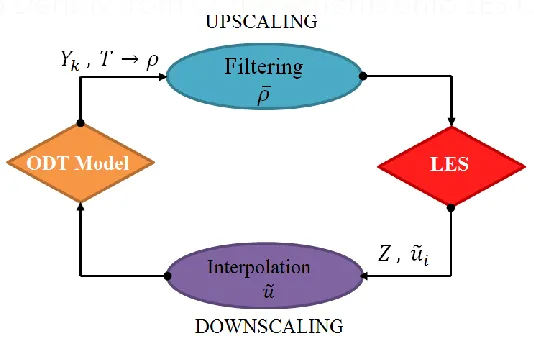
Figure 4.1 Coupling of LES with ODT and passing information between two solvers .. 27
Figure 5.1 A schematic illustration of LES-ODT computational grid ... 31
Figure 5.2.a The LES cell and ODT element attached to the flame surface in 3D ... 34
Figure 5.2.b The relative positions of the ODT grid point and LES cell in influenced region ... 34
Figure 5.3.a Effective domain adopted for filtering ... 35
Figure 5.3.b Effective domain oriented in the direction normal to the flame surface ... 35
Figure 5.4 Blending pure mixing solution and filtered density based on ODT solution . 37 Figure 5.5 Smoothing function used for blending the density from LES-ODT and pure mixing solution ... 39
Figure 5.6 Flow chart of proposed spatially filtering density for LES-ODT ... 40
Figure 6.1 A schematic of the computational domain... 45
Figure 6.2.a Growth of the flame brush and attached ODT elements at simulation time of 0.18s ... 49
Figure 6.2.b Growth of the flame brush and attached ODT elements at simulation time of 0.20s ... 49
Figure 6.3 Contribution of the ODT domains to each LES cell in filtering process ... 49
Figure 6.4 Overlapping ODT elements on NCWF contour ... 50
Figure 6.5 Temperature field at solution time step of 590 ... 51
Figure 6.6 Temperature field at solution time step of 650 ... 51
Figure 6.7 FDS density field ... 52
Figure 6.8 Filtered density... 52
Figure 6.9 Temperature field at 22s ... 53
Figure A.1 Tri-Linear interpolation for a cell ... 60
CHAPTER 1
Introduction
1.1.
Background
Summary of Comparing the Methods
1.1.In RANS, all the scales from integral scales up to dissipation range needs to be modeled.
1.2.In LES, part of the inertial sub range and the beginning of the dissipation scales is modeled.
1.3.In DNS, no modeling needs to be done but it solves resolution for all the range, i.e., from the large scales completely through dissipation scales.
1.2.
Motivation
1.3.
Objective
1.4.
Chapters Outline
The following topics are divided into 6 chapters:
Chapter 2: Review and Discussion of One Dimensional Turbulence
Chapter 3: The Large Eddy Simulation and Fire Dynamics Simulator
Chapter 4: Multi-scale Flame-Embedding LES-ODT Strategy
Chapter 5: Case Study and Density Spatial Filtering
CHAPTER 2
One-Dimensional Turbulence
In this chapter, the One Dimensional Turbulence (ODT) model is introduced. The approach and governing equations is reviewed briefly and at the end, the application of the method in flame-embedding model is discussed. Its objective is to model a strategy for coupling of turbulent transport, diffusion and reaction processes. This model can be applied to simple turbulent flows evolving temporally and spatially [6].
2.1.
Introduction
In summary, one-dimensional domains in ODT consider [7]:
Chemistry
Stirring (advective) Events
Molecular transport (diffusion)
2.2
Governing Equations
In this section the governing equations for ODT are briefly reviewed. The equations are relevant to the present Lagrangian formulation where ODT solutions are advected along the flame surface. Note that turbulent transport is modeled stochastically whereas reaction and diffusion processes are implemented deterministically. An in-depth discussion of formulation and model has been presented in [6] and [7].
In the present formulation, the LES-ODT solution involves the advection of numerous ODT domains or elements along the flame. The advection is based on the filtered velocity, while the effects of the fluctuating components of the velocity are implemented as part of the ODT elements’ solution. The ODT domains are identified with their anchor points and their orientation, which is maintained normal to the flame. The anchor moves at the fluid filtered velocity, ̅, suchthattheanchor’spositioncanbeupdatedusing[6]:
̅ (2.1)
written into two components; filtered (resolved) component, ̃, and residual component, . The former component is being modeled in LES and it is related to the large-scale transport; whereas the latter component accounts for the simulation of ODT turbulent stirring events.
̃ (2.2)
In summary the ODT governing equations for each one-dimensional element are:
Conservation of Momentum
(
) (2.3)
Conservation of Energy
[ (
) ̇ ] (2.4)
Conservation of Species
[ (
) ̇ ] (2.5)
Also the equation of state for ideal gas is as follow:
Ideal Gas Equation of State
(2.6)
Term ̇ in equations (2.4) and (2.5) refers to the source term due to reaction and the stochastic process is shown with . Note that is the coordinate on the ODT elements normal to the flame surface. Mean advection terms are not appeared in the equations above yet they have a stretching role for the flame, which should be taken into consideration. The turbulence process modeling in the governing equations ( ) are modeled stochastically using the “triplet maps” method. Modeling of the stirring event in ODT starts with the appropriate selection of Eddy size, location, rate of distribution and probability computation and ends with the triplet map [16].
2.3
ODT Scalars Calculation
In the previous section, the one-dimensional-turbulence governing equations were discussed. This section is focused on computing the values for the scalars appeared in equations (2.3) through (2.6), which is in accordance to with Fire Dynamics Simulator open source code. The viscosity, material diffusivity and thermal conductivity are approximated from kinetic theory since the temperature dependence of each plays an important role in combustion. For the present study, the chemistry is a one-step reaction mechanism of propane and oxygen. Having said that, the reaction between the fuel (C3H8) and oxidizer (O2) can be written as:
2.3.1 Density
The equation of state for ideal gas is written to compute the density for each species in the computational domain. The specific gas constant can be expressed in terms of universal gas constant, mass fraction and molecular weight of each species. Thus
(2.8)
and
∑ (2.9)
where is the universal gas constant,
, is the mass fraction and is the molecular weight of the species. Note that in equation (2.8), pressure is constant throughout this case study and temperature and mass fraction are the resolved by One-Dimensional Turbulence governing equations.
2.3.2 Mass Diffusivity
Diffusion refers to the instantaneous mixing resulted from the existence of the species concentration gradient. It can be shown that the mass diffusivity ( ) of a binary system is a function of temperature, pressure and composition. For multicomponent gas mixtures, Chapman-Enskog Theory [14], the binary diffusion coefficient ( ⁄ ) can be written as:
√
This equation states the dependence of the diffusion coefficient on the temperature and species. In the equation below:
:“Collisiondiameter”,aLennard-Jones parameter ( )
(2.11)
:“Diffusioncollisionintegral”,dimensionless;referto[15] and [16]. ̃ ̃ ̃
̃ (2.12) and
̃
(2.13)
In the equation above, ̃ is a dimensionless temperature which is represented in terms of absolute temperature , Boltzmann’s constant ( 1.381 10-23 ⁄ ) and a characteristic mixture energy parameter. This characteristic can be estimated in terms of the Lennard-Jones (12-6) potential characteristic energies for species A and B ( ):
√ (2.14)
Values of for different species are provided in Poling et al. (2000) [16].
can be obtained using:
( )
(2.15)
2.3.3 Gaseous Mixture Viscosity
complicated. There are several interpolative methods: Reichenberg, Wilke, Herning and Zipperer are among these methods. In this study, the method suggested by Chung et al. is used to estimate the mixture viscosity. )Poling et al. [16]).
⁄ (2.16)
where is the Lennard-Jones hard-sphere diameter and is analogous to a molecular diameter, on the other hand is viscosity collision integral and it is obtained from the empirical equation below proposed by Neufeld et al. [15]:
( ̃) ̃ ̃ (2.17)
The gaseous mixture viscosity is given by:
∑ (2.18)
2.3.4 Specific Heat Capacity
The constant pressure specific heat of the mixture is obtained from:
∑ (2.19)
where is the temperature dependent specific heat of species .
2.3.5 Thermal Conductivity
The thermal conductivity of species is given by:
(2.20)
On a side note, one assumption here is considering the nitrogen as dominant species in any combustion scenario and therefore the diffusion coefficient in the species mass conservation equation is that of the given species diffusion into nitrogen[17]:
(2.21)
2.3.6 Mass Production Rate
The chemical mass production rate of species per unit volume for fuel (C3H8) and oxidizer (O2) in equations (2.4), (2.5) are obtained from the equations (2.22),(2.23) below. As a convention, the subscript “ ” is used for fuel and “ ” to denote the oxidizer.
̇ ( ) (2.22)
̇ ̇ (2.23)
and represent the pre-exponential factor, activation energy and mole fraction of
CHAPTER 3
Large-Eddy Simulation and Fire Dynamics
Simulator
3.1
Introduction
Large-Eddy Simulation is a powerful method amongst the turbulence numerical simulation methods. The LES technique is increasingly becoming major tool for modeling combustion. It aims at computing the large scale effects directly while the small scales are modeled. The former scales are influenced by geometry and responsible for turbulent transport of heat and momentum, whereas the latter scales are universal in the flow field. Note that small scales are not universal for chemistry. In LES the small effects are filtered out yet their influence on the large-scale motions is statistically introduced [22] and [24]. By filtering the governing equations, unclosed terms appear and need to be addressed. The unresolved turbulent fluxes can be modeled by providing closure terms. In this chapter, LES governing equations are presented. Filtering and closuring strategies are briefly discussed. Some features of Fire Dynamics Simulator such as Combustion Model are reviewed.
3.2
Large-Eddy Simulation
LES models the unsteady large scale mixing instead of averaging it.
LES is capable of predicting the instabilities emerging from the coupling between hydrodynamic flow field and heat release.
LES computes the large-scale effects explicitly, which mostly depend on the geometry. In contrast, the small scales events are universal properties and thus turbulence modeling of the smallest scale structures can make it efficient and justifiable for combustion flows.
3.2.1 Filtering
As noted earlier, the governing equations are spatially filtered either in the physical space or spectral space. The filtering in LES corresponds to applying a low-pass filter. The filtered operation is expressed as:
̅ ∫ (3.1)
where represents the LES filter.
All the filters are normalized, which implies:
∫ ∫ ∫ (3.2)
A mass-weighted filter also can be defined as:
̅ ̃ ∫ (3.3)
The filter above is called, Favre filtering. Common filters are: the cut-off filter, the box filter, the Gaussian filter, and the Cauchy filter [24].
In turbulent flows, any instantaneous quantity ( ) might be decomposed into a filtered component (̅) and a fluctuating component ( ).
̅ (3.5)
In order to make a distinction between different types of filtering, the Favre Average is denotedby“ ̃ ”andfilteredquantityareshownby“ ̅ ”.
In the next section, the LES governing equations are presented.
3.2.2 Governing Equations
By filtering the instantaneous governing equations for fluid flow, the LES equations are obtained:
Conservation of Mass
̅
̅ ̃
(3.6)
Conservation of Momentum
̅ ̃
( ̅ ̃ ̃ )
̅
( ̅ ) ̅ (3.7)
Conservation of Mixture Fraction
Conservation of Energy ( ̅ ̃ ) ( ̅ ̃ ̃ ) [ ̅( ̃ ̃ ̃ )] ̅ ̇̅
̇̅ ̇̅ ̅ (3.9)
Ideal Gas Equation of State
̅ ̅ (3.10)
In equation (3.8), is the subgrid scale Schmidt number and is the subgrid scale viscosity computed from Smagorinsky model Equations (3.7)-(3.9) contain unclosed (unresolved) terms such as:
(3.7): unclosed Reynolds Stress – subgrid scale turbulence model used as
closure
(3.9): unclosed enthalpy fluxes ̅( ̃ ̃ ̃ ) and average dissipative rate ̅
In equation (3.7), represents the subgrid scale (SGS) stress and is expressed as equation (3.13) in the next section. Note that ̇̅ , ̇̅ and ̇̅ stated in (3.9) represent heat fluxes due to conduction and radiation, and heat release rate per unit volume, and heat transfer to evaporating droplets. Each can be computed as follows:
̇̅
∑
̇̅ (3.11)
3.2.3 Closure
By filtering the governing equations, there are terms that remain unresolved and require closure to be modeled. Since combustion occurs at the unclosed scales of the computations, addressing closure plays important role in combustion models. The scope of closures is beyond the current study; nonetheless, the closure terms used in the approach are worth to present.
The subgrid stress can be expressed as:
̅( ̃ ̃ ̃ ) (3.13)
Smagorinsky model, [25], offers a gradient-diffusion model to represent the subgrid transport. The eddy viscosity model provides a closure term for unresolved momentum flux [26]: [( ) ] (3.14)
The equation above can also be written in terms of subgrid scale viscosity ( and symmetric strain tensor ( ):
(3.15)
where symmetric strain tensor is defined as:
(
) (3.16)
and is the Kronecker delta.
(3.17)
It is important to realize that LES models the dissipative processes due to viscosity, thermal conductivity and material diffusivity happens at scales smaller than those that are explicitly resolved on the numerical grid. In other word, viscosity, thermal conductivity and diffusivity cannot be expressed directly. In the Smagorinsky model, the viscosity can be modeled as:
( ̅ ̅ ( ̅
) ) (3.18)
In this equation, is a characteristic length corresponding to the filter size, and is an empirical constant. Note the bar over the quantities above indicates that they are computed on a numerical grid. Thermal conductivity and diffusivity are given by:
(3.19)
(3.20)
3.3
Fire Dynamics Simulator
practical fire problems and serving as a resource for combustion studies such as sprinkler, heat detector, flame spread and fire growth[17].
3.3.1 Features and Assumptions
The main features of the FDS code include: a hydrodynamic model, a combustion model and radiation transport. Here, only a brief description is provided. Details can be found in [17]. FDS computes the governing equations with rectilinear grids. In FDS, the hydrodynamic boundary conditions near the wall uses the empirical correlation based on Werner and Wengle model, ([27] and [28]), whereas the solid surfaces are set as thermal boundary conditions and the empirical correlations are applied for the heat and mass transfer to and from solid surfaces.
3.3.2 Hydrodynamic Model
FDS uses a low-Mach number formulation for the solution of the Navier-Stokes equations for low-speed and thermally driven flow. The equations are based on the LES approach. The numerical scheme is explicit and has second order accuracy temporally and spatially. As mentioned earlier, the Smagorinsky model uses a gradient-diffusion model to represent the subgrid transport.
3.3.3 Radiation Transport
3.3.4 Combustion Model
The mixture fraction concept is implemented in FDS combustion model. The mixture fraction (Z) is defined as the ratio of mass of material having its origin in the fuel stream to the mass of mixture. The mass fraction canbeobtainedbythe“Staterelations”fromthe mixture fractions (Figure 3.1). Note that mixture fraction is a conserved scalar. The mixture fraction-based combustion model is used for LES. This model is according to the Arrhenius reaction rate for each species, i.e. infinitely fast chemistry kinetics. Theterm“fast”implies that reactions occur so quick that there is no co-existence circumstance for fuel and oxidizer. The latter is presented in the following section.
The model used in the present study postulates a single-step, instantaneous reaction. This reaction of fuel and oxygen can be written as:
CαHβOγNaMb + O2 CO2 + H2O + CO + S + N2 + M (3.21)
In the reaction above, shows the soot which is a mixture of carbon and hydrogen, is the stoichiometric coefficient, represents the additional products and are the number of the atoms in the fuel molecule. Hence, the mixture fraction can be expressed as:
(
) ( ) ( ) (3.22)
it yields:
(
Since the mixture fraction is a function of time and space, it is expressed as . The flame surface is where the oxidizer and fuel meet under stoichiometric conditions. The assumption of fast chemistry implies the fuel and oxidizer vanish at flame surface:
(3.24)
in which:
(3.25)
In equations above, is the stoichiometric mixture fraction, is mass fraction in oxidizer supply, is the mass fraction in fuel supply and .
The mixture fraction in equation (3.23) can be rewritten into two components and :
(3.26)
(
) ( ) ( ) (3.27)
(3.28)
There are circumstances in which the fuel and the oxygen may mix but not burn. This intricate situation may be predicted based on the concentration and temperature of the gases adjacent to the flame surface. The partitioning of terms into two components helps to understand if the condition is met for the reaction to happen. Therefore, for describing the composition of the mixture at least two scalar variables are required. In the equation above,
Figure 3.1 State relations for propane [30]
Figure 3.2 Oxygen-temperature phase space presenting where combustion is allowed or not allowed to take place[30]
Mixture Fraction (Z)
M a ss F ra ct io n (Y )
0 0.2 0.4 0.6 0.8 1
0 0.2 0.4 0.6 0.8 1 N2
Fuel (C3H8)
O2
H2O
CO2
Zf=Zstoichiometric
Gas Temperature (oC)
O x y g en V o lu m e F ra ct io n (% )
0 500 1000 1500
Accordingly, the species mass fraction in the mixture can be found by:
(3.37)
(3.29)
(3.30)
(3.31)
(3.32)
(3.33)
(3.34)
(3.35)
(3.38)
(3.39)
(3.40)
(3.41)
(3.42)
CHAPTER 4
LES-ODT Model and Implementation
In this chapter, the model based on Large-Eddy Simulation and One-Dimensional Turbulence is reviewed. The coupling of the governing equations and passing data between the two solvers are discussed. Then, the implementation of the model in the proposed flame-embedding approach is presented.
4.1 LES-ODT Framework and Passing Information
mass fractions. The ODT scalars such as density, mass diffusivity, gaseous mixture viscosity, thermal conductivity, etc. are calculated as described in the previous chapter. These properties are estimated based on the kinetic theory where properties are temperature dependent. The velocity and mixture fraction are interpolated from LES into ODT domains by tri-linear interpolation scheme (Appendix A). The LES velocity substitutes the large-scale component of the ODT velocity. The governing equations along the ODT domains are solved. The flame structure is resolved by ODT model.
Figure 4.1 Coupling of LES with ODT and passing the information between two solvers
LES. Modeling of the stirring event in ODT starts with the selection of eddy size and position and ends with the triplet map[11].
Note that ODT domains are advected through their anchor point. The anchor point velocity for each ODT domain can be calculated from LES velocity field as follows:
̃
(4.1)
CHAPTER 5
Density Filtering Procedure
This chapter is devoted to an approach developed to spatially filter the information from high-resolution one-dimensional-turbulence model grids, attached to flame brush, to the coarse grid of Large-Eddy-Simulation. In particular, the aim of density filtering presented here is to provide LES solver with the density attained from ODT solver by filtering it into LES cells. Although the primary focus of the approach is on filtering the density, this algorithm can be applied to the source terms as well. Moreover, the strategy is followed by smoothing step and blending the ODT solutions filtered into LES cells and the pure-mixing LES solution computed in Fire Dynamics Simulator right before passing the data to LES solver.
5.1
Overview
approach; nevertheless it can be a case study for further investigation by introducing the proper modifications. In the current study, an algorithm is developed and implemented in order to pass the density to the LES solver. The spatial filter scheme exploits the Gaussian Cubature Method. Additionally, the implemented method is optimized to perform the task without any further cost of computation. Finally, a density blending scheme is introduced to obtain a smooth density throughout the entire domain by combining density from ODT with density from the FDS solution of pure mixing outside the flame. In the following sections, the steps above are discussed in details and the case study and simulation results are presented in Chapter 6.
5.2
Spatial Filtering (Upscaling)
Figure 5.1 A schematic illustration of LES-ODT computational grid. Subfigure (a) presents the 3D flame brush and coarse grid of LES Subfigure (b) shows a 2D cross section of the domain Subfigure (c) illustrates a closer look at high resolution ODT domain attached to flame brush
The leftmost Figure (a) shows the flame brush at a specific simulation time as delineated by the stoichiometric value of the filtered mixture fraction. Each ODT grid point on the one-dimensional elements is carrying evaluated information such as density . Each ODT domain can be represented by its end-points. Similarly every point on the ODT domain can be specified by its position in the Cartesian coordinate system. The number of ODT points on each element determines the resolution of the subgrid solver. As described earlier, the surface of the flame can be computed by the mixture fraction Z corresponding to the stoichiometric condition. The solution for the mixture fraction is carried out in LES solver. All the embedded elements are oriented in the direction normal to the flame brush and fixed via the anchor point. In Figure (b) the ODT elements are shown. Due to the higher resolution of the ODT grids, every LES cell adjacent to the elements includes lines of ODT
points. Thus, the effect of each ODT grid point has to be taken into account and this contribution should be modeled. In particular, this contribution is not only due to the number of the ODT points present within a LES cell but also should be a function of their distance to LES cell center. The proposed spatial filtering method uses a distance-based weighting function called the cubature method. Furthermore, several tasks and corresponding algorithm are developed to reduce the cost of the computation. These tasks include pre-filtering the density on each ODT domain, applying the Gaussian as the kernel function for the cubature method, introducing cut-off for the Gaussian function, and eventually investigation and using a function for blending and smoothing the density attained from ODT and FDS.
In the subsequent sections below, the developed scheme is discussed in detail. The scheme is validated by simple test cases. Eventually, the approach is implemented in the LES-ODT flame-embedding approach and the density field is passed to LES as discussed earlier.
5.2.1 The Gaussian Cubature Method
A principal implementation of the spatial filter relies on the method of cubature. Each LES cell is allotted a contribution from ODT grid point in its vicinity. As stated in the previous section, this contribution is related to the distance of the LES cell center and the ODT grid point ( ). This distance can be found from relations (B.7) to (B.10) in Appendix B.
∫ ̅ ∫ (5.1)
Note the weighting of each ODT grid point on the adjacent LES cells decays as a function of its distance from any LES grid center. A Gaussian weighting function is introduced as the kernel function in cubature method in the above equation. The integrand and general equation for the Cubature Method for the scalar (density here) can be written as:
(5.2)
∫ ̅ ∫ (5.3)
In equation above, the kernel function is the Gaussian weighting function and the left hand side is called Gaussian Weighted Integral (known as Gaussian Cubature Method) [19]. Since the domain is discretized, the summation is substituted over the computational domain.
∑ ̅ ∑ (5.4)
This procedure is applied in order to spatially filter the density (it can be another source term also) onto the LES cells. The equation (5.4) above can be rewritten as:
̅ (∑ ) (∑ ) (5.5)
ODT point, and ̅ is the filtered density onto LES cell center. Thus, the process has an upscaling behavior.
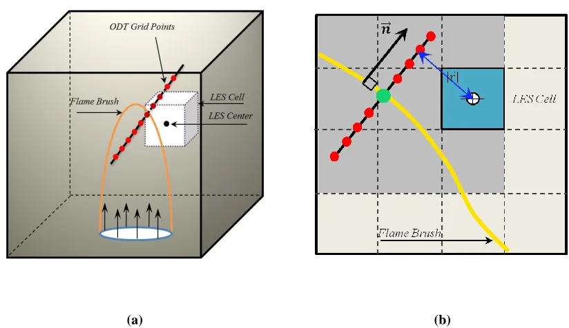
Figure 5.2 (a) The LES cell and ODT Element attached to the flame surface in 3D
(b) The relative positions of the ODT Grid Point and LES cell in influenced region
This is demonstrated in Figure 5.2. Every LES cell in the influenced region around the ODT domain is captured as discussed in next section below and the corresponding weighting factor, , and weighted density, , are tagged within each cell.
5.2.2 Influence Domain and Effective Radius
The proposed spatial filtering exploits a region of influence around each high resolution ODT element. The LES cells that are distant from the ODT elements have a negligible contribution from ODT grid points. Therefore, LES grids are simply discarded by a cut-off
Gaussian kernel function in filtering process; therefore, the cost of computation is significantly decreased. The criteria defined for the influenced domain would be restricted to a dimensionless radius called an effective radius. The locus of all LES center points located in a specific distance from ODT element implies a cylindrical effective region of influence around each ODT elements. Therefore, a cylindrical coordinate system is chosen so that its axis is oriented in the normal direction to the flame surface (shown in Figure 5.3). Note that the effective radius is of the order of the ODT element length and defined by:
(5.6)
The two hemispheric regions attached to the cylinder, shown in Figure (a), account for the ending effects of each one-dimensional turbulence domains. Figure (b) exhibits the ODT
(a) (b)
Figure 5.3 (a) Effective domain adopted for filtering
domain enclosed by the region of influence and cylindrical coordinate system used for filtering. Having said that, the Cut-Off Gaussian as a kernel function is formulated as below:
(5.7)
In the equation (5.7), defines a secondary scaling factor by which the rate of decaying Gaussian kernel function is controlled. This factor is equivalent of having more ODT domains involved in filtering procedure and defines an effective bandwidth for filtering.
5.2.3 Blending of the Filtered Density Solutions
In the previous section, the scheme for upscaling the density from One-Dimensional Turbulence model into LES grid was discussed. Since the ODT elements are placed near the flame and the filtering may not implemented away from the flame, blending of the LES filtered density solution with a non-reacting density solution from LES is needed to cover the entire LES computational domain. The filtered density ( ) is mapped onto the density obtained by pure mixing solution ( ). A blending method is implemented in order to blend the solution at the overlapped region (Figure 5.4). This is done by introducing an average cell properties based on a blending function, .
(5.8)
Figure 5.4 Blending pure mixing solution and filtered density based on ODT solution
The blending function is a non- dimensional parameter that is interpreted as a measure of confidence in the availability of adequate ODT data to determine the ODT-based filtered density. Therefore, it is evaluated based on the accumulated weighting, ∑ , of filtered density in each LES cell:
∑ |
(5.9)
(5.10)
is evaluated at each upscaled LES cell. According to this value and a smoothing function below, is determined. is indeed a measure for contribution of spatially filtered density and FDS density; close to 1 indicates that there is a significant contribution of ODT points in the cell, and thus, it has to have a higher contribution to LES solution than FDS solution in that particular cell.
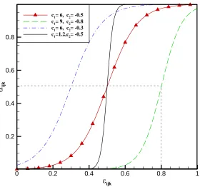
A bounded smoothing function below is postulated in a general form of:
(5.12) The function has a domain and range in interval whereas constants and are responsible for the stretching/compressing and sliding of the smoothing function.
Hence, an array of are computed during the spatial filtering of the density and is evaluated by equation (5.12) in transition from attained ODT solution adjacent to the flame surface to the FDS solution around.
The Figure 5.6 illustrates the flow chart for the filtering process.
Figure 5.5
Smoothing function used for blending the density from LES-ODT and FDS solution ijk
ijk
0 0.2 0.4 0.6 0.8 1
0.2 0.4 0.6 0.8
CHAPTER 6
LES-ODT Simulation: Non-Premixed Propane –
Air Jet Flame
6.1
Objectives
In this chapter, the LES-ODT flame-embedding approach is used to simulate a turbulent non-premixed propane-air jet flame. First, the simulation conditions are presented. Then, the governing equations specific to the problem is reviewed. The implementation of the developed algorithm and strategy is discussed. The filtered density field is presented at 3 different simulation time. The trend of scalars such as density, temperature, fuel mass fraction and oxidizer mass fraction along an ODT domain are exhibited. The effect of finite chemistry on temperature is presented.
6.2
Simulation Conditions
The simulation of non-premixed propane-air flame jet uses a one-step reaction mechanism of propane (C3H8) and (O2) oxygen as follows:
C3H8 + 5(O2 + 3.76 N2) 3 CO2 + 4 H2O + 18.8 N2
6.2.1 Governing Equations for LES-ODT Flame-Embedding Approach
LES Governing Equations:
Conservation of Mass
̅
̅ ̃
(6.1)
Conservation of Momentum
̅ ̃
( ̅ ̃ ̃ )
̅
( ̅ ) ̅ (6.2)
Conservation of Mixture Fraction
̅ ̃ ̅ ̃ ̃ ( ̅ ̃ ) (6.3)
ODT Governing Equations:
Conservation of Momentum
(
Conservation of Energy
[ (
) ̇ ] (6.5)
Conservation of Species for Oxidizer
[ (
) ̇ ] (6.6)
Conservation of Species for Fuel
[ (
) ̇ ] (6.7)
Ideal Gas Equation of State
(6.8)
6.2.2 Boundary Conditions and Geometry
The computational domain for the current simulation and the run conditions are presented in table 6.1 below. As it is illustrated in Figure 6.1, the domain is open to atmospheric pressure and has an inlet at the bottom. In the inlet, propane jet is injected with a co-flow of air at different velocities as described.
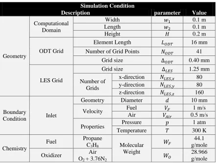
Table 6.1 Simulation Conditions for Non-premixed Turbulent Flame
Simulation Condition
Description parameter Value
Geometry
Computational Domain
Width 0.1 m
Length 0.1 m
Height 0.2 m
ODT Grid
Element Length 16 mm
Number of Grid Points 41
Grid size 0.40 mm
LES Grid
Grid size 1.25 mm
Number of Grids
x-direction 80 y-direction 80 z-direction 160
Boundary
Condition Inlet
Geometry Diameter 10 mm
Velocity Fuel 1 m/s
Air 0.5 m/s
Properties Pressure 1 atm
Temperature 300 K
Chemistry
Fuel Propane
C3H8 Molecular Weight
44.1 g/mole
Oxidizer Air
O2 + 3.76N2
28.966 g/mole
the grid size for LES domain specifies the resolution of the coarse grid used for Large Eddy Simulation.
Figure 6.1 A schematic of the computational domain
6.2.3 Model Implementation
flame is not fully developed, introducing the ODT elements is postponed until the flame has evolved. Afterwards, the ODT elements are attached to the flame brush at their anchor points. The flame surface is defined by the stoichiometric mixture fraction computed in FDS. This step is accompanied by the coupling and exchange of information between LES and ODT model. The ODT governing equations require the downscaled velocity and mixture fraction from LES. The downscaling process is performed by tri-linear interpolations from the LES grids to the ODT grids. This method estimates the value of an intermediate point within a cubical element (see Appendix B, [8], [9]). The anchor points are moved and developed as the flame is tracked. As the simulation time elapses, the number of ODT domains and their orientation will change.
Stirring events are implemented by performing triplet maps. Once the ODT governing equations are solved at a LES time step, the density is filtered to LES grids. The filtering process at each time step, as described in the previous chapter, consists of several stages. These stages are:
1. The calculation of the temperature and mass fraction from mixture fraction provided by the LES solution
2. The calculation of the density at each ODT grid point 3. The tagging of the LES cells influenced by ODT domain 4. Book-keeping the distance of each LES cell and ODT elements
5. The recording of the coordinate of the projected LES cell on ODT element
8. The calculation of filtered density
9. The smoothing of the solution by finding the contribution of the filtered density for LES cells and the FDS density
10.Finally, the density is passed to the LES solver and the coupling cycle continues
6.3
Results
In this section, the results of the LES-ODT simulation of a turbulent non-premixed propane-air jet flame are presented. The evolution of the flame is shown at different time steps. The arrangement of the ODT domains attached to the surface is presented. The fuel mass fraction, oxidizer mass fraction, temperature and density over an ODT domain are shown. The tagged LES cells captured in density filtering are shown. Finally, the smooth filtered density is exhibited.
The surface of the flame corresponds to the mixture fraction in stoichiometric condition, which is for propane and air is = 0.059. Each ODT element is oriented in the direction normal to the flame surface. This normal unit vector is given by:
⃗
| | (6.9)
(a) (b)
Figure 6.2 (a) Growth of flame brush and ODT elements attached at simulation time: 0.18s
(b) Growth of flame brush and ODT elements attached at simulation time: 0.20s
Figure 6.4 Overlapping ODT elements on NCWF contour ( )
Figure 6.5 Temperature field at solution step 590
In Figures 6.7 and 6.8, the FDS density and spatially filtered density are shown. Note that the solution obtained from the filtered density has filtered some of the peaks as expected since filtering is a volume averaging process. Given the inverse relation between temperature and density in the ideal gas equation, the higher temperature corresponds to a lower density and vice versa. Thus, as it can be seen the peaks are filtered out in the spatially filtered density filed.
CHAPTER 7
Conclusion and Future Work
7.1
Conclusion
In this study, an approach for spatially filtering the density for flame-embedding using LES-ODT is developed. The Lagrangian embedding strategy is used for the simulation of a non-premixed flame. The LES model and ODT model are coupled in this framework. The small- scale effects are captured using the ODT high-resolution domains. The coupling and passing of the information between the two models is demonstrated. The upscaling of the density from ODT to LES is investigated and an algorithm is developed. The simple one-step air-propane reaction is modeled as a case study. The proposed filtering scheme for density completes the coupling step of LES-ODT approach for flame-embedding strategy.
7.2
Future Work
REFERENCES
[1] Kuo, Kenneth K., Yun Acharya, R., ”Fundamentals of Turbulent and Multi-Phase Combustion”, Wiley, 2012
[2] Pope, Stephen B., “Turbulent Flows”, Cambridge University Press, 2000 [3] Beyssiere, V., Jarosinski, J., “Combustion Phenomena”, CRC Press, 2009 [4] Peters, N., “Turbulent Combustion”, Cambridge University Press, 2000
[5] Poinsot, T, Veynante, D., “Theoretical and Numerical Combustion”, 2nd Edition, R. T. Edwards(Ed.), 2005
[6] Echekki, T., “Turbulent Combustion Modeling: Advances, New Trends and Perspectives”, Springer, 2011
[7] Cao, S., Echekki, T., “A Low-Dimensional Stochastic Closure Model for Combustion Large-Eddy Simulation”, Journal of Turbulence, 58(24): 1-35, 2008 [8] Sedhai, S., Echekki, T., “An ODT-Based Flame-Embedding Approach for
Turbulent Non-Premixed Combustion”, AIAA, 2012
[9] Sedhai, S., “A Multiscale Flame-Embedding Framework for Turbulent Combustion using LES-ODT”,Master’sthesis,NorthCarolinaStateUniversity,2011
[10] Balasubramanian, S., “ Novel Approach for the Direct Simulation of Subgrid-Scale Physics in Fire Simulations”,Master’sthesis,NorthCarolinaStateUniversity, 2010 [11] Kerstein, A. R., “One Dimensional Turbulence: Model Formulation and
[12] Punati Kumar, N., “An Eulerian One-Dimensional Turbulence Model: Application to Turbulent and Multiphase Reacting Flows”, PhD thesis, University of Utah, 2012 [13] Ricks, A.J., Hewson, J.C., Kerstein, A.R., Gore, J.P., Tieszen, S.R., Ashurst, W.T.,
“A Spatially-developing One Dimensional Turbulence Study of Soot and Enthalpy Evolution in Meter-scale Buoyant Turbulent Flames”, Combustion Science Technology, 182:60-101, 2010
[14] Chapman, S., Cowling, T. G., The Mathematical Theory of Non-uniform gases: an Account of the Kinetic Theory of Viscosity, Thermal Conduction and Diffusion in Gases”, 3rd
Edition, Cambridge University Press, 1970
[15] Neufield, P. D., Jansen, A. R., Aziz, R. A., “Empirical Equations to Calculate 16 of the Transport Collision Integrals for the Lennard-Jones (12-6) Potential”, Journal of Chemical Physics,57:1100-1102, 1972
[16] Poling,B.E.,Prausnitz,O’Connell,J.P.,“The Properties of Gases and Liquids”, 5th Edition, McGraw-Hill, 2001
[17] McGrattan, K., Hostikka, S., Floyd, J., Baum, H., Rehm, R., “Fire Dynamics Simulator (Version 5) Technical Reference Guide”, NIST (National Institute of Standards and Technology), 2007
[18] Puri, I., Seshadri, K., “Extinction of Diffusion Flames Burning Diluted Methane and Diluted Propane in Diluted Air”, Combustion and Flame, 65:137, 1996
[20] Press W. H., Teukolsky, S. A., Vetterling, W. T., Flannery, B. P., “Numerical Recipes in Fortran”, Cambridge University Press, 2nd
Edition, 1996
[21] Wesseling, P., “Principles of Computational Fluid Dynamics”, Springer-Verlag Berlin Heidelberg, 2001
[22] Hanifi, A., Alfredsson, P. H., Johansson, A. V., Henningson, D. S., “Transition, Turbulence and Combustion Modelling”, Kluwer Academic Publishers, 1998
[23] Pitsch, H., “Large-Eddy Simulation of Turbulent Combustion”, Annual Review of Fluid Mechanics, 38:453-482, 2006
[24] Vervisch, L., Veynante, D., J. van Beeck, J.P.A., “Turbulent Combustion, Lecture Series 2009-07”, von Karman Institute for Fluid Dynamics, 2009
[25] Smagorinsky, J., “General Circulation Experiments with the Primitive Equations”, Monthly Weather Review, 91:99-164, 1963
[26] Meneveau, C., “Turbulence: Subgrid-Scale Modeling”, Scholarpedia, 5:9489, 2010 [27] Werner, H., Wengle, H., “Large-Eddy Simulation of Turbulent Flow around a Cube
in a Plane Channel”, Turbulent Shear Flows Symposium, Springer, 8:155-68, 1993 [28] Piomelli, U., “Wall-Layer Models for Large-Eddy Simulations”, Progress in
Aerospace Sciences, 4: 437-446, 2008
[29] Hergert, W., Wriedt, T., “The Mie Theory, Basics and Applications”, Springer Series in Optical Sciences, 2012
Appendix A
Tri-linear Interpolation
Downscaling the scalars from LES grid to ODT grid exploits tri-linear interpolation. These scalars addressed in the coupled LES-ODT methodology are mixture fraction and velocity [20], [21]. These scales are resolved by LES governing equations. In a sense, downscaling the scalars stands opposite to filtering and upscaling the information.
Figure A.1 Tri-linear interpolation for a cell
In the prism above, it is assumed that each node has an assigned value. If point were tagged with index , then would be the corresponding
values at node . To interpolate the value at arbitrary point , within the cell above, method of tri-linear is used. The cell can be divided in to 8 volumes by planes defined by . These volumes can be normalized by dividing them by the total volume of the cell.
(A.1)
(A.2)
(A.3)
Appendix B
Note on Spatial Filtering
Here the basic concept and its formulation are proofed.
Imagine line in 3D space, represents the ODT element attached to the flame surface. The procedure is set based on finding the distance of the LES cell center and the ODT element. The foot of the perpendicular on the line can be obtained. The corresponding distance of each LES cell center to the ODT grid point the element is calculated. Note that the line has a normal vector, ⃗ and can be obtained from the corresponding stoichiometric mixture fraction.
Figure B.1 Finding distance between LES cell center and ODT element
(B.1)
| ⃗⃗⃗⃗⃗⃗⃗⃗⃗⃗ | (B.2)
(B.4) (B.5)
⃗⃗⃗⃗ ⃗⃗⃗⃗⃗⃗⃗⃗⃗⃗ (B.6)
( ) ( ) ( ) (B.7) Also: ( ) (B.8)
( ) (B.9)
Inserting (B.8) and (B.9) into (B.7) yields . Hence, the foot of perpendicular point is known.
| ⃗⃗⃗⃗ | √ (B.10)
(B.11)
If the resolution of the ODT domain is denoted by and the number of the domains by , then ODT density can be represented as follows:
(
)
specific ODT domain which the distance is calculated. This array is used to find the weighting of each ODT domain in each adjacent LES cell centers.
This array for the ODT number can be written as:
Corresponding to , an array can be defined based on Gaussian Cubature Method for each LES cell. The accumulated weight and density for each cell is computed.
∑
(B.12)
Hence,
̅ ( ∑
) ( ∑
![Figure 3.1 State relations for propane [30]](https://thumb-us.123doks.com/thumbv2/123dok_us/1322590.1165137/33.612.186.428.371.588/figure-state-relations-for-propane.webp)