Electromagnetic interrogation and the Doppler shift using the method of mappings

(1)

Electromagnetic Interrogation and the Doppler

Shift Using the Method of Mappings

H.T. Banks, Shuhua Hu and W. Clayton Thompson

Center for Research in Scientiﬁc Computation

North Carolina State University

Raleigh, NC 27695-8212

December 11, 2009

Abstract

We consider the electromagnetic detection of hidden moving or oscillating conductive targets. The resulting mathematical problem involves computation of a Doppler shift for an electromagnetic wave reflecting from a moving interface. This entails solving Maxwell’s equations on a domain changing in time. We employ the method of mappings to transform the problem to one of computing solutions of a Maxwell system with time dependent coef-ficients on a fixed reference domain. Thus we obtain a problem that is eminently tractable with finite element or finite difference time domain methods. Accuracy of numerical solu-tions is illustrated with computasolu-tions for a number of different velocities for the moving interface.

AMS subject classiﬁcations: 35Q61,83C50,83C22,65M32.

(2)

1 Introduction

We consider the general problem ofelectromagnetic interrogation ofa moving interface. In particular we are interested in the frequency shift (double Doppler shift) for an interrogating wave reﬂected from a moving conductive material target or interface. Such problems were ﬁrst considered in 1905 by Einstein [8] in early work on relativity theory and have continued to be of interest in subsequent years [7, 9] especially in the context ofmodern radar technology (e.g., see [6, 9, 10] and the numerous references therein). In a number of applications the moving target may be one of detection in that the target is hidden or masked by a dielectric material (e.g., buried targets such as land mines, improvised explosive devices, etc., internal organs or implants or protheses, internal aircraft or automotive engine components). The targets ofinterest may be moving due to external disturbances (such as elastic waves as used in seismic exploration, acoustic waves as used in medical probes) or natural vibrations (e.g., rotating aircraft engine compressor blades, contracting/expanding arteries in compressed or normal blood circulation). In any case, for many such examples the mathematical problem is rather simply stated: one must analyze Maxwell’s equations on a moving domain, i.e., a domain with moving boundaries or interfaces.

The classical approach often encountered in the literature (and described briefly below) makes use of the Lorentz transformation from relativity theory–see for example [6]. Related approaches (e.g., see [7, 9]) assume undamped time harmonic wave fields incident on a moving plane interface and determine reflection properties via boundary interface conditions. An approach that does not involve the Lorentz transformation includes that of [10] which is based on differentiation of interface conditions at moving boundaries and combining these with Maxwell’s equations. This approach however still involves use offinite differences or finite elements on moving domains.

The ideas presented here in the context ofthe mathematical framework of[3] are based on the so-calledmethod of mappingstechniques frequently encountered in domain or shape optimization problems [11] that also have been used for example in thermal interrogation problems [4, 5] as well as in electromagnetic interrogation [3]. The ideas as illustrated here in a one dimensional setting are rather simply stated: one maps a constant (in time) coefficient partial differential equation (e.g., Maxwell’s equations) given on a time changing or moving domain to a partial differential equation with time-dependent coefficients but on a fixed reference domain. The resulting prob-lems are thus quite suitable for solution by finite difference or finite element numerical methods. This approach is not restricted to simple rectilinear movement ofthe interfaces or boundaries. The approach is simple, requires no relativistic transformations and can in principle, be used in interrogation problems for complex moving targets in higher dimensions when combined with perfectly matched layer (PML) formulations [1, 2]. Our primary requirement is that the moving interface or target be defined by an 𝐻2 _{time dependent boundary. We describe the ideas in}

(3)

2 General Case

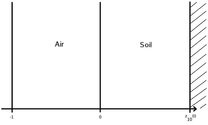
We illustrate the basic ideas in the context of the framework developed in [3]. We formulate a mathematical model governing the electric field intensity ofa polarized electromagnetic pulse emitted by an antenna as it propagates from air to a dielectric (we use parameters for soil here), partially reflects and partially transmits at the air/dielectric interface, propagates through the dielectric and then reflects from a perfectly conducting surface (the target), and propagates back to the air. We will consider the geometry shown in Figure 1. The positive 𝑧 axis extends to the right in the figure; the air-soil interface is fixed at 𝑧 = 0 while the target (assumed to be a perfect conductor) is mobile, with position given by 𝑧10(𝑡) (assumed>0). The left boundary of

the domain (where we will place a source current) without loss ofgenerality is assumed to be at

𝑧 =−1.

Figure 1: Geometry ofthe 1D mathematical model for EM interrogation.

With this geometry, we may now write the governing equation [3] for the electric ﬁeld on the domain𝑧 ∈[−1, 𝑧10(𝑡)], 𝑡≥0. For 𝑧 ∈[−1,0], we have the standard Maxwell’s equation

∂2_𝐸₍_{𝑡, 𝑧}₎

∂𝑡2 −𝑐2

∂2_𝐸₍_{𝑡, 𝑧}₎

∂𝑧2 =−

1

𝜖0

∂𝐽𝑠(𝑡, 𝑧)

(4)

Here we do not distinguish air from a vacuum. For𝑧 ∈[0, 𝑧10(𝑡)], we have

𝜖𝑟∂

2_𝐸₍_{𝑡, 𝑧}₎

∂𝑡2 +

1

𝜖0

(

𝜎(𝑧) +𝑔(0, 𝑧))∂𝐸_∂𝑡(𝑡, 𝑧)

+ _𝜖1

0

(

∂𝑔(𝑡, 𝑧)

∂𝑡 𝐸(0, 𝑧) +

∫ _𝑡

0

∂𝑔(𝑡−𝑠, 𝑧)

∂𝑡

∂𝐸(𝑠, 𝑧)

∂𝑠 𝑑𝑠

)

− 𝑐2∂2𝐸(𝑡, 𝑧)

∂𝑧2 =−

1

𝜖0

∂𝐽𝑠(𝑡, 𝑧)

∂𝑡 .

(2)

These equations have been adapted from [3, eqn (2.14)]; here 𝜖𝑟 = _𝜖𝜖

0 is the relative permittivity

ofthe dielectric, 𝜎(𝑧) is the conductivity ofsoil, 𝑔(𝑡, 𝑧) is the polarization susceptibility kernel, and 𝐽𝑠(𝑡, 𝑧) is the source current. We make two simplifying assumptions. First, the soil is

assumed to be uniform throughout, so that𝜎(𝑧) =𝜎. Second, we assume that the source current is emitted from a point at the left boundary of the spatial domain and has the form

𝐽𝑠(𝑡, 𝑧) =𝛿(𝑧+ 1)𝑗(𝑡), (3)

where𝑗(𝑡) is a function to be speciﬁed and𝛿 is the Dirac delta distribution with support at {0}. We assume that the electric ﬁeld intensity is initially zero and static so that the initial conditions are

𝐸(0, 𝑧) = 0

∂𝐸

∂𝑡 (0, 𝑧) = 0,

for 𝑧 ∈ [−1, 𝑧10(𝑡)]. We assume that the target is a perfect conductor and that there is no

reﬂection from the left boundary (absorbing boundary conditions). Thus the boundary conditions

are [

1

𝑐 ∂𝐸

∂𝑡 − ∂𝐸

∂𝑧

]

𝑧=−1

= 0

𝐸(𝑡, 𝑧10(𝑡)) = 0.

For this problem the domain on which the equations hold [−1, 𝑧10(𝑡)] is time-varying. Hence

(5)

2.1 Method of Mappings

Given the function 𝑧10(𝑡), we consider the change ofvariables (𝑡, 𝑧)→(𝜏, 𝜁) deﬁned by

𝜁(𝑡, 𝑧) =

{ _𝑧, _𝑧 _≤₀

𝑧

𝑧10(𝑡), 𝑧 >0

𝜏(𝑡) = 𝑡,

with inverse transformation

𝑧(𝜏, 𝜁) = {

𝜁, 𝜁 ≤0

𝜁𝑧10(𝜏), 𝜁 >0

𝑡(𝜏) = 𝜏.

It is easy to verify that the transformation is locally invertible provided 𝑧10(𝑡) ∕= 0, which we

have already assumed. Moreover, it maps the domain [−1, 𝑧10(𝑡)] to the ﬁxed reference domain

[−1,1]. We now undertake the task oftransforming the original system (in𝐸(𝑡, 𝑧) on [−1, 𝑧10(𝑡)])

into an equivalent system deﬁned in terms of ˜𝐸(𝜏, 𝜁) on [−1,1] where

𝐸(𝑡, 𝑧) = ˜𝐸(𝜏(𝑡), 𝜁(𝑡, 𝑧)).

For𝑧 ≤0, the transformation is simply a change of notation, and yields

∂2_𝐸˜₍_{𝜏, 𝜁}₎

∂𝜏2 −𝑐2

∂2_𝐸˜₍_{𝜏, 𝜁}₎

∂𝜁2 =−

𝛿(𝜁+ 1)

𝜖0

∂𝑗(𝜏)

∂𝜏 . (4)

For 𝑧 > 0, we invoke the chain rule for each of the derivatives appearing in (2). For the state variable, we have

∂𝐸 ∂𝑧 =

∂𝐸˜ ∂𝜁

∂𝜁 ∂𝑧 =

∂𝐸˜ ∂𝜁

1

𝑧10(𝑡). (5)

Continuing to the second derivative with respect to the state variable, we obtain

∂2_𝐸

∂𝑧2 =

∂ ∂𝑧

[ 1

𝑧10(𝑡)

∂𝐸˜ ∂𝜁

] = ∂

∂𝜁

[ 1

𝑧10(𝑡)

∂𝐸˜ ∂𝜁

]

∂𝜁 ∂𝑧 =

1

𝑧2 10(𝑡)

∂2_𝐸˜

∂𝜁2. (6)

For the time variable, we ﬁnd

∂𝐸 ∂𝑡 =

∂𝐸˜ ∂𝜏

∂𝜏 ∂𝑡 +

∂𝐸˜ ∂𝜁

∂𝜁 ∂𝑡

= ∂_∂𝜏𝐸˜ − ∂_∂𝜁𝐸˜

(

𝑧 𝑧2

10(𝑡)

∂𝑧10(𝑡)

∂𝑡

)

.

(6)

Continuing for the second derivative, we have

∂2_𝐸

∂𝑡2 =

∂ ∂𝑡 [ ∂𝐸˜ ∂𝜏 − ∂𝐸˜ ∂𝜁 ( 𝑧 𝑧2

10(𝑡)

∂𝑧10(𝑡)

∂𝑡 )] = _∂𝜏∂ [ ∂𝐸˜ ∂𝜏 ] ∂𝜏 ∂𝑡 + ∂ ∂𝜁 [ ∂𝐸˜ ∂𝜏 ] ∂𝜁 ∂𝑡 − ∂ ∂𝑡 [ ∂𝐸˜ ∂𝜁 ( 𝑧 𝑧2

10(𝑡)

∂𝑧10(𝑡)

∂𝑡

)]

= ∂_∂𝜏2𝐸˜₂ − _{∂𝜁∂𝜏}∂2𝐸˜

(

𝑧 𝑧2

10(𝑡)

∂𝑧10(𝑡)

∂𝑡 ) − ∂_∂𝜁𝐸˜_∂𝑡∂ [ 𝑧 𝑧2

10(𝑡)

∂𝑧10(𝑡)

∂𝑡

]

−_𝑧₂𝑧

10(𝑡)

∂𝑧10(𝑡)

∂𝑡 ∂ ∂𝑡 [ ∂𝐸˜ ∂𝜁 ]

= ∂_∂𝜏2𝐸˜₂ − _{∂𝜁∂𝜏}∂2𝐸˜

(

𝑧 𝑧2

10(𝑡)

∂𝑧10(𝑡)

∂𝑡

)

− ∂_∂𝜁𝐸˜

(

∂𝑧10(𝑡)

∂𝑡

−2𝑧 𝑧3

10(𝑡)

∂𝑧10(𝑡)

∂𝑡 + 𝑧 𝑧2

10(𝑡)

∂2_𝑧 10(𝑡)

∂𝑡2

)

−_𝑧₂𝑧

10(𝑡)

∂𝑧10(𝑡)

∂𝑡 ( ∂ ∂𝜏 [ ∂𝐸˜ ∂𝜁 ] ∂𝜏 ∂𝑡 + ∂ ∂𝜁 [ ∂𝐸˜ ∂𝜁 ] ∂𝜁 ∂𝑡 )

= ∂_∂𝜏2𝐸˜₂ −2_{∂𝜁∂𝜏}∂2𝐸˜ (

𝑧 𝑧2

10(𝑡)

∂𝑧10(𝑡)

∂𝑡 ) +∂_∂𝜁𝐸˜ [ 2𝑧 𝑧3

10(𝑡)

(

∂𝑧10(𝑡)

∂𝑡

)2

− _𝑧₂𝑧

10(𝑡)

∂2_𝑧 10(𝑡)

∂𝑡2

]

+∂_∂𝜁2𝐸˜₂ (

𝑧 𝑧2

10(𝑡)

∂𝑧10(𝑡)

∂𝑡

)₂

. (8)

Replacing the variables 𝑧 and 𝑡 where they appear in Equations (5) - (8) with 𝜁𝑧10(𝜏) and 𝜏

respectively, we ﬁnd

∂𝐸 ∂𝑡 = ∂𝐸˜ ∂𝜏 − ∂𝐸˜ ∂𝜁 ( 𝜁 𝑧10(𝜏)

∂𝑧10(𝜏)

∂𝜏

)

(9)

∂2_𝐸

∂𝑡2 =

∂2_𝐸˜

∂𝜏2 −2

∂2_𝐸˜

∂𝜁∂𝜏

(

𝜁 𝑧10(𝜏)

∂𝑧10(𝜏)

∂𝜏 ) +∂_∂𝜁𝐸˜ [ 2𝜁 𝑧2

10(𝜏)

(

∂𝑧10(𝜏)

∂𝜏

)₂

− _𝑧 𝜁

10(𝜏)

∂2_𝑧 10(𝜏)

∂𝜏2

]

+∂_∂𝜁2𝐸˜₂ (

𝜁 𝑧10(𝜏)

∂𝑧10(𝜏)

∂𝜏 )2 (10) ∂𝐸 ∂𝑧 = ∂𝐸˜ ∂𝜁 1

𝑧10(𝜏) (11)

∂2_𝐸

∂𝑧2 =

1

𝑧2 10(𝜏)

∂2_𝐸˜

∂𝜁2. (12)

We observe that 𝐸(0, 𝑧) = ˜𝐸(𝜏(0), 𝜁(0, 𝑧)) = ˜𝐸(0, 𝜁) for all 𝑧. We also need a means of treating the polarization kernel 𝑔(𝑡, 𝑧) in the original formulation. To this end we deﬁne ˜𝑔 via

(7)

consider the transformation of the function 𝑔 when 𝑧 >0. Thus ∂𝑔 ∂𝑡 = ∂𝑔˜ ∂𝜏 ∂𝜏 ∂𝑡 + ∂𝑔˜ ∂𝜁 ∂𝜁 ∂𝑡 = ∂_∂𝜏𝑔˜− ∂_∂𝜁𝑔˜ ( 𝑧 𝑧2

10(𝑡)

∂𝑧10(𝑡)

∂𝑡

)

= ∂_∂𝜏𝑔˜− ∂_∂𝜁𝑔˜

(

𝜁 𝑧10(𝜏)

∂𝑧10(𝜏)

∂𝜏

)

.

(13)

We are ﬁnally ready to substitute these expressions (9)-(13) into (2) and obtain

𝜖 𝜖0

[

∂2_𝐸˜

∂𝜏2 − 2

∂2_𝐸˜

∂𝜁∂𝜏

(

𝜁 𝑧10(𝜏)

∂𝑧10(𝜏)

∂𝜏 ) +∂_∂𝜁𝐸˜ ( 2𝜁 𝑧2

10(𝜏)

(

∂𝑧10(𝜏)

∂𝜏

)2

− _𝑧 𝜁

10(𝜏)

∂2_𝑧 10(𝜏)

∂𝜏2

)

+ ∂_∂𝜁2𝐸˜₂ (

𝜁 𝑧10(𝜏)

∂𝑧10(𝜏)

∂𝜏

)₂] +_𝜖1

0

(

𝜎+ ˜𝑔(0, 𝜁)) [∂_∂𝜏𝐸˜ −∂_∂𝜁𝐸˜

(

𝜁 𝑧10(𝜏)

∂𝑧10(𝜏)

∂𝜏

)]

+_𝜖1

0 ∫ _𝜏 0 ( ∂˜𝑔(𝜏−𝑠, 𝜁) ∂𝜏 − ∂˜𝑔(𝜏−𝑠, 𝜁) ∂𝜁 𝜁 𝑧10(𝜏 −𝑠)

∂𝑧10(𝜏 −𝑠)

∂𝜏 ) ( ∂𝐸˜(𝑠, 𝜁) ∂𝑠 − ∂𝐸˜(𝑠, 𝜁) ∂𝜁 ( 𝜁 𝑧10(𝑠)

∂𝑧10(𝑠)

∂𝑠

))

𝑑𝑠

+_𝜖1

0 ( ∂𝑔˜ ∂𝜏 − ∂𝑔˜ ∂𝜁 𝜁 𝑧10(𝜏)

∂𝑧10(𝜏)

∂𝜏

) ˜

𝐸(0, 𝜁)−𝑐2 1

𝑧2 10(𝜏)

∂2_𝐸˜

∂𝜁2 = 0,

(14)

for 𝜏 ≥ 0 and𝜁 ∈ [0,1]. Observe that the right side ofthe equation is zero because the source current is zero in the given domain. Together with (4), (14) provides a piecewise set ofequations for ˜𝐸. It follows trivially that the new initial conditions are

˜

𝐸(0, 𝜁) = 0

∂

∂𝜏𝐸˜(0, 𝜁) = 0,

(15)

and the boundary conditions are [ 1 𝑐 ∂𝐸˜ ∂𝜏 − ∂𝐸˜ ∂𝜁 ]

𝜁=−1

= 0

˜

𝐸(𝜏,1) = 0.

(16)

(8)

3 A Special Case: The Case without Dissipation

In order to validate and demonstrate the application ofthe method ofmappings technique, we consider a simpliﬁed problem equivalent to that discussed by Van Bladel in [6, Sec 5.9]. We assume as in [6] a time-harmonic plane wave in a vacuum is normally incident on a perfect conductor which is moving with constant velocity parallel to the direction ofwave propagation. Thus the need to consider dispersion or polarization in the soil is removed (𝜎 = 0, 𝑔(𝑡, 𝑧) = 0). The position ofthe target is𝑧10(𝑡) =𝑣𝑧𝑡+𝑧0 where 𝑣𝑧 is the velocity ofthe target and 𝑧0 is its

position at𝑡 = 0. We will also assume that the source current is sinusoidal in time,𝑗(𝑡) = sin(𝜔𝑡).

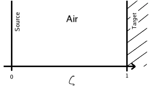
Figure 2: Geometry ofthe undamped problem in the 𝜁 coordinate.

This problem is well-known from basic relativistic considerations (as shown in [6, Sec 5.9]) to produce a so-called “double Doppler shift”, so that the frequency of the wave reﬂected from the conductor is

𝑓𝑟 =𝑓𝑖1_{1 +}−𝑣_𝑣𝑧/𝑐

𝑧/𝑐, (17)

where𝑓𝑖 denotes the frequency of incident wave. The derivation is based on the Lorentz

transfor-mation from classical relativity theory. We now seek to use the method ofmappings to recreate this result computationally and thus demonstrate the eﬃcacy ofthe proposed method. For sim-plicity, we will only consider the electric ﬁeld on the domain 𝑧 ∈[0, 𝑧10(𝑡)] (the vacuum will not

change the wave form, so moving the left boundary from 𝑧 =−1 to 𝑧 = 0 does not change the problem; the source current will thus be𝐽𝑠(𝑡, 𝑧) =𝛿(𝑧) sin(𝜔𝑡)). After the appropriate change of

variables, the new geometry for this special case is shown in Figure 2 and the governing equation is

∂2_𝐸˜₍_{𝜏, 𝜁}₎

∂𝜏2 − 2

∂2_𝐸˜₍_{𝜏, 𝜁}₎

∂𝜁∂𝜏

(

𝑣𝑧𝜁

𝑣𝑧𝜏 +𝑧0

)

+∂𝐸˜_∂𝜁(𝜏, 𝜁) [

2𝑣2

𝑧𝜁

(𝑣𝑧𝜏 +𝑧0)2

]

− ∂2𝐸˜_∂𝜁(𝜏, 𝜁₂ )

(

𝑐2₋_𝑣2

𝑧𝜁2

(𝑣𝑧𝜏+𝑧0)2

)

=−_𝜖𝜔

0𝛿(𝜁𝑧10(𝜏)) cos(𝜔𝜏),

(9)

with boundary conditions _[ 1

𝑐 ∂𝐸˜

∂𝜏 −

1

𝑧10(𝜏)

∂𝐸˜ ∂𝜁

]

𝜁=0

= 0

˜

𝐸(𝜏,1) = 0.

(19)

The initial conditions are still given by (15).

3.1 Weak/Variational Formulation

We next proceed to write (18) and (19) into variational form in preparation for the introduction ofnumerical approximations. Deﬁne

𝛼(𝜏, 𝜁) = _𝑣 2𝑣𝑧𝜁

𝑧𝜏 +𝑧0, 𝛽(𝜏, 𝜁) =

2𝑣2

𝑧𝜁

(𝑣𝑧𝜏+𝑧0)2, 𝛾(𝜏, 𝜁) =

𝑐2₋_𝑣2

𝑧𝜁2

(𝑣𝑧𝜏+𝑧0)2.

Let⟨⋅,⋅⟩be the standard𝐿2₍₀_,_{1) inner product and let} _𝜙_∈_𝐻1

𝑅(0,1)≡ {𝜙∈𝐻1(0,1)∣𝜙(1) = 0}.

Then

〈

∂2_𝐸˜₍_𝜏,_⋅₎

∂𝜏2 , 𝜙

〉

−

〈

𝛼(𝜏,⋅)∂2_{∂𝜏∂𝜁}𝐸˜(𝜏,⋅), 𝜙

〉 +

〈

𝛽(𝜏,⋅)∂𝐸˜_∂𝜁(𝜏,⋅), 𝜙

〉

−

〈

𝛾(𝜏,⋅)∂2𝐸_∂𝜁˜(𝜏,₂ ⋅), 𝜙

〉 =

〈

−_𝜖𝜔

0𝛿(𝜁𝑧10(𝜏)) cos(𝜔𝜏), 𝜙

〉

.

(20)

We then use integration by parts on the fourth term of (20). In our subsequent discussions, we let (′_{) be the} ∂

∂𝜁 derivative and (˙) be the ∂

∂𝜏 derivative: we have

〈

𝛾(𝜏,⋅)∂2𝐸˜(𝜏,⋅)

∂𝜁2 , 𝜙

〉

= 𝛾(𝜏, 𝜁)𝜙(𝜁)∂𝐸˜(𝜏, 𝜁)

∂𝜁

1

0

−

∫ ₁

0

∂𝐸˜(𝜏, 𝜁)

∂𝜁 (𝛾(𝜏, 𝜁)𝜙′(𝜁) +𝛾′(𝜏, 𝜁)𝜙(𝜁))𝑑𝜁

=−𝛾(𝜏,0)𝜙(0)∂𝐸˜_∂𝜁(𝜏,0)−

〈

∂𝐸˜

∂𝜁 , 𝛾(𝜏,⋅)𝜙′+𝛾′(𝜏,⋅)𝜙

〉

.

(21)

For the source current term, we ﬁnd 〈

−_𝜖𝜔

0𝛿(𝜁𝑧10(𝜏)) cos(𝜔𝜏), 𝜙

〉

=−_𝜖 𝜔

(10)

Substituting (21) and (22) into (20), we obtain 〈

∂2_𝐸˜₍_𝜏,_⋅₎

∂𝜏2 , 𝜙

〉

−

〈

𝛼(𝜏,⋅)∂2_{∂𝜏∂𝜁}𝐸˜(𝜏,⋅), 𝜙

〉 +

〈

𝛽(𝜏,⋅)∂𝐸˜_∂𝜁(𝜏,⋅), 𝜙

〉

+𝛾(𝜏,0)𝜙(0)∂𝐸˜_∂𝜁(𝜏,0)

+ 〈

∂𝐸˜(𝜏,⋅)

∂𝜁 , 𝛾(𝜏,⋅)𝜙′+𝛾′(𝜏,⋅)𝜙

〉

=−_𝜖 𝜔

0𝑧10(𝜏)cos(𝜔𝜏)𝜙(0). (23)

Now observe that

𝛾(𝜏,0)𝜙(0)∂𝐸˜(𝜏,0)

∂𝜁 −

1

𝑐𝛾(𝜏,0)𝜙(0)𝑧10(𝜏)

∂𝐸˜(𝜏,0)

∂𝜏

= −𝛾(𝜏,0)𝜙(0)𝑧10(𝜏)

[ 1

𝑐 ∂𝐸˜

∂𝜏 −

1

𝑧10(𝜏)

∂𝐸˜ ∂𝜁

]

𝜁=0

= 0

by the boundary condition at 𝜁 = 0. Thus the resulting variational form is 〈

∂2_𝐸˜₍_𝜏,_⋅₎

∂𝜏2 , 𝜙

〉

−

〈

𝛼(𝜏,⋅)∂2_{∂𝜏∂𝜁}𝐸˜(𝜏,⋅), 𝜙

〉 +

〈

𝛽(𝜏,⋅)∂𝐸˜_∂𝜁(𝜏,⋅), 𝜙

〉

+1_𝑐𝛾(𝜏,0)𝜙(0)𝑧10(𝜏)∂

˜

𝐸(𝜏,0)

∂𝜏 +

〈

∂𝐸˜(𝜏,⋅)

∂𝜁 , 𝛾(𝜏,⋅)𝜙′+𝛾′(𝜏,⋅)𝜙

〉

=−_𝜖 𝜔

0𝑧10(𝜏)cos(𝜔𝜏)𝜙(0).

(24)

The functions𝛼(𝜏, 𝜁),𝛽(𝜏, 𝜁), and𝛾(𝜏, 𝜁) are real valued and the weak derivative𝛾′ _{can be easily}

computed analytically.

3.2 Finite Elements Method

To solve (24), we use ﬁrst order ﬁnite elements methods (FEM). We assume that the𝜁domain has been partitioned into an evenly spaced grid (step size ℎ) with nodes 𝜁𝑘, 𝑘 = 0, . . . , 𝑁 (𝜁𝑘=ℎ𝑘).

We then deﬁne the ‘hat’ functions (piecewise linear splines)

𝜙0(𝜁) =

{ _𝜁

1−𝜁

ℎ , 𝜁 ≤𝜁1

0, 𝑜𝑡ℎ𝑒𝑟𝑤𝑖𝑠𝑒 ,

𝜙𝑖(𝜁) =

⎧    ⎨    ⎩

𝜁−𝜁𝑖−1

ℎ , 𝜁𝑖−1 ≤𝜁 ≤𝜁𝑖 𝜁𝑖+1−𝜁

ℎ , 𝜁𝑖 ≤𝜁 ≤𝜁𝑖+1

0, 𝑜𝑡ℎ𝑒𝑟𝑤𝑖𝑠𝑒

(11)

Following standard FEM technique, we assume that the solution to (24) can be approximated as

˜

𝐸(𝜏, 𝜁)≈𝐸˜𝑁₍_{𝜏, 𝜁}₎_≡𝑁∑−1 𝑖=0

𝑤𝑖(𝜏)𝜙𝑖(𝜁),

where the 𝑁 coeﬃcient functions𝑤𝑖(𝜏) are now the unknowns to be determined via (24). With

these substitutions into equation (24), we now have an inﬁnite number ofequations in 𝑁 un-knowns (recall that (24) must hold for all𝜙 ∈𝐻1

𝑅(0,1)). In order to form a uniquely determinable

system ofequations, we let𝜙(𝜁) =𝜙𝑗(𝜁),𝑗 = 0, . . . , 𝑁−1, in turn. Then for each𝑗 = 0, . . . , 𝑁−1,

we must have

𝑁−1

∑

𝑖=0

¨

𝑤𝑖(𝜏)⟨𝜙𝑖, 𝜙𝑗⟩ − 𝑁_∑−1

𝑖=0

˙

𝑤𝑖(𝜏)⟨𝛼(𝜏,⋅)𝜙′𝑖, 𝜙𝑗⟩+ 𝑁_∑−1

𝑖=0

𝑤𝑖(𝜏)⟨𝛽(𝜏,⋅)𝜙′𝑖, 𝜙𝑗⟩

+ 1_𝑐𝛾(𝜏,0)𝜙𝑗(0)𝑧10(𝜏) ˙𝑤0(𝜏) +

𝑁−1

∑

𝑖=0

𝑤𝑖(𝜏)⟨𝜙′𝑖, 𝛾(𝜏,⋅)𝜙′𝑗⟩

+

𝑁_∑−1

𝑖=0

𝑤𝑖(𝜏)⟨𝜙′𝑖, 𝛾′(𝜏,⋅)𝜙𝑗⟩=−_𝜖 𝜔

0𝑧10(𝜏)cos(𝜔𝜏)𝜙𝑗(0).

(25)

This constitutes 𝑁 equations for the 𝑁 unknowns 𝑤𝑖, 𝑖 = 0,1, . . . , 𝑁 −1. It is also useful to

compute the following:

⟨𝜙𝑖, 𝜙𝑗⟩= ⎧   ⎨   ⎩

ℎ/3, 𝑖=𝑗 = 0 2ℎ/3, 𝑖=𝑗 ∕= 0

ℎ/6, ∣𝑖−𝑗∣= 1 0, 𝑜𝑡ℎ𝑒𝑟𝑤𝑖𝑠𝑒

(26) ⟨𝛼(𝜏,⋅)𝜙′ 𝑖, 𝜙𝑗⟩= ⎧            ⎨            ⎩ −𝑣𝑧ℎ

3(𝑣𝑧𝜏 +𝑧0), 𝑖=𝑗 = 0

−2𝑣𝑧ℎ

3(𝑣𝑧𝜏 +𝑧0), 𝑖=𝑗 ∕= 0

𝑣𝑧(3𝑖−2)ℎ

3(𝑣𝑧𝜏 +𝑧0), 𝑖=𝑗+ 1

−𝑣𝑧(3𝑖+ 2)ℎ

3(𝑣𝑧𝜏 +𝑧0) , 𝑖=𝑗−1

(27) ⟨𝛽(𝜏,⋅)𝜙′ 𝑖, 𝜙𝑗⟩= ⎧             ⎨             ⎩ −𝑣2 𝑧ℎ

3(𝑣𝑧𝜏 +𝑧0)2, 𝑖=𝑗 = 0

−2𝑣2

𝑧ℎ

3(𝑣𝑧𝜏 +𝑧0)2, 𝑖=𝑗 ∕= 0

𝑣2

𝑧(3𝑖−2)ℎ

3(𝑣𝑧𝜏 +𝑧0)2, 𝑖=𝑗+ 1

−𝑣2

𝑧(3𝑖+ 2)ℎ

3(𝑣𝑧𝜏 +𝑧0)2 , 𝑖=𝑗−1

(12)

⟨𝜙′ 𝑖, 𝛾(𝜏,⋅)𝜙′𝑗⟩= ⎧             ⎨             ⎩

3𝑐2₋_𝑣2

𝑧ℎ2

3ℎ(𝑣𝑧𝜏+𝑧0)2, 𝑖=𝑗 = 0

6𝑐2₋₂_𝑣2

𝑧ℎ2(3𝑖2+ 1)

3ℎ(𝑣𝑧𝜏+𝑧0)2 , 𝑖=𝑗 ∕= 0

𝑣2

𝑧ℎ2(3𝑖2−3𝑖+ 1)−3𝑐2

3ℎ(𝑣𝑧𝜏+𝑧0)2 , 𝑖=𝑗+ 1

𝑣2

𝑧ℎ2(3𝑖2+ 3𝑖+ 1)−3𝑐2

3ℎ(𝑣𝑧𝜏+𝑧0)2 , 𝑖=𝑗 −1

, (29) ⟨𝜙′ 𝑖, 𝛾′(𝜏,⋅)𝜙𝑗⟩= ⎧             ⎨             ⎩ 𝑣2 𝑧ℎ

3(𝑣𝑧𝜏 +𝑧0)2, 𝑖=𝑗 = 0

2𝑣2

𝑧ℎ

3(𝑣𝑧𝜏 +𝑧0)2, 𝑖=𝑗 ∕= 0

−𝑣2

𝑧ℎ(3𝑖−2)

3(𝑣𝑧𝜏 +𝑧0)2 , 𝑖=𝑗+ 1

𝑣2

𝑧ℎ(3𝑖+ 2)

3(𝑣𝑧𝜏 +𝑧0)2, 𝑖=𝑗−1

. (30)

Let w𝑁₍_𝜏_{) = (}_𝑤

0(𝜏), 𝑤1(𝜏), . . . , 𝑤𝑁−1(𝜏))𝑇. Then it follows that we can write (25) as a vector

system with 𝑁 equations in 𝑁 variables

𝑀w¨𝑁₍_𝜏_{) +}

(

𝑐 𝑣𝑧𝜏+𝑧0ee

𝑇 ₋_𝐶₍_𝜏₎

) ˙

w𝑁₍_𝜏_{) + (}_𝐾

1(𝜏) +𝐾2(𝜏) +𝐾3(𝜏))w𝑁(𝜏) =𝐹(𝜏), (31)

where the (𝑖, 𝑗)th element of𝑀, 𝐶,𝐾1,𝐾2, and𝐾3 are deﬁned in (26), (27), (28), (29) and (30),

respectively, e is a 𝑁-dimensional column vector with a one as its ﬁrst component and zeros otherwise, and 𝐹(𝜏) is a 𝑁-dimensional column vector given by

𝐹(𝜏) = (

−_𝜖 𝜔

0𝑧10(𝜏)cos(𝜔𝜏),0,0, . . . ,0

)_𝑇

.

Thus (31) is a vector ordinary diﬀerential equation for the vector coeﬃcient functionw𝑁 _which

can readily be solved numerically.

3.3 Computational Results

We ﬁrst present results at high velocity to clearly demonstrate the accuracy ofthe method ofmappings compared with that ofclassical electromagnetic Doppler shift computations. In carrying out the computations, we assume 𝑧0 = 2. The electromagnetic source is truncated at

𝑡 = 𝑡∗ _{= 4}_𝜋/𝜔 _{so that only two sinusoidal pulses are emitted and reﬂected (this makes the}

(13)

The following notation will be used throughout the remainder ofthis presentation: 𝑓𝑖,𝑎𝑛𝑙

denotes the frequency of the incident wave with which we interrogate the system (we use 1e+9 Hz in all calculations here), 𝑓𝑖,𝑠𝑖𝑚 is the corresponding frequency obtained by simulation. Similarly,

we use 𝑓𝑟,𝑎𝑛𝑙 and 𝑓𝑟,𝑠𝑖𝑚 to represent the frequency of reﬂected waves obtained by using the Van

Bladel formula (17) and simulation, respectively. Then the frequency shift obtained by the Van Bladel formula and simulation are calculated by

Δ𝑓𝑎𝑛𝑙 =∣𝑓𝑖,𝑎𝑛𝑙−𝑓𝑟,𝑎𝑛𝑙∣, and Δ𝑓𝑠𝑖𝑚 =∣𝑓𝑖,𝑠𝑖𝑚−𝑓𝑟,𝑠𝑖𝑚∣,

respectively. The relative error Rel𝑖 for the incident wave is calculated by

Rel𝑖 = 100∣𝑓𝑖,𝑎𝑛𝑙_𝑓−𝑓𝑖,𝑠𝑖𝑚∣ 𝑖,𝑎𝑛𝑙 .

Similarly, the relative error for the reﬂected wave and for the frequency shift are obtained by

Rel𝑟= 100∣𝑓𝑟,𝑎𝑛𝑙_𝑓−𝑓𝑟,𝑠𝑖𝑚∣

𝑟,𝑎𝑛𝑙 , and Rel𝑠 = 100

∣Δ𝑓𝑎𝑛𝑙−Δ𝑓𝑠𝑖𝑚∣

Δ𝑓𝑎𝑛𝑙 ,

respectively.

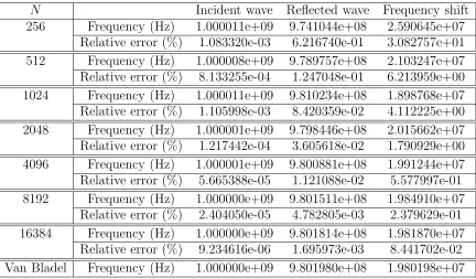
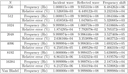
In Figure 3, the magnitude ofthe electric ﬁeld is shown as a function oftime at a chosen value of𝑧(𝑧 = 0.3), where the results are obtained with𝑣𝑧 = 3×103 and𝑁 = 16384. In the top graph,

the incident wave moves past𝑧= 0.3 followed at some time later by the reflected wave. These two waves are magnified in the lower two graphs. Even though the electric field𝐸 has discontinuous derivative (w.r.t 𝑧) at the leading edges ofthe waves, numerical Gibbs type oscillations at these leading edges are resolved by using sufficiently large values of 𝑁 (see [3] for discussions). The data displayed in the graph can be used to estimate the period (and hence the frequency) of the waves as shown in the figure. Using this data, the estimated frequency of the incident wave is

𝑓𝑖,𝑠𝑖𝑚 = 999.999MHz, and the relative error for incident wave is Rel𝑖 ≈6.21×10−6% (see Table

5). The estimated frequency of the reﬂected wave is 𝑓𝑟,𝑠𝑖𝑚 ≈999.978MHz with the relative error

Rel𝑟 being around 1.93×10−4%. The estimated frequency shift is Δ𝑓𝑠𝑖𝑚 ≈ .02187MHz with

relative error Rel𝑠 being around 8.56%.

To see the eﬀect ofthe values of𝑣𝑧 and 𝑁 on the accuracy of the obtained frequency shift,

we illustrated the results for𝑓𝑖,𝑎𝑛𝑙,𝑓𝑖,𝑠𝑖𝑚,𝑓𝑟,𝑎𝑛𝑙, 𝑓𝑟,𝑠𝑖𝑚, Δ𝑓𝑎𝑛𝑙, Δ𝑓𝑠𝑖𝑚, Rel𝑖, Rel𝑟 and Rel𝑠 obtained

by using diﬀerent target velocity 𝑣𝑧 (varied from 3×107 to 3×103) as well as diﬀerent number

𝑁 of spline functions (varied from 256 to 16384) in Tables 1-5. From these tables we can see that the relative error for the reﬂected wave (Rel𝑟) decreases as 𝑁 increases. In addition, the

frequency of reﬂected wave obtained by simulation (𝑓𝑟,𝑠𝑖𝑚) is very close to that obtained by the

Van Bladel formula (𝑓𝑟,𝑎𝑛𝑙) for all the 𝑁’s and velocities that we have tried. For example, even

(14)

0 0.2 0.4 0.6 0.8 1 1.2 1.4 1.6 1.8 2

x 10−8

−150 −100 −50 0 50 100 150

E(t,z

obs), vz=3000, N=16384

Time, t

Electric Field Magnitude

0.5 1 1.5 2 2.5 3

x 10−9 −150

−100 −50 0 50 100 150

Incident Wave

Time, t

1.2 1.25 1.3 1.35 1.4 1.45

x 10−8 −150

−100 −50 0 50 100 150

Reflected Wave

Time, t

Figure 3: Electric field magnitude at 𝑧 = 0.3 as a function of time. The incident and reflected waves are both visible in the top graphic and are magnified in the bottom graphics. The under-lying data can be used to estimate the periods ofthe waves, and hence their frequencies.

We also observed that the relative error for the frequency shift (Rel𝑠) decreases as𝑁 increases.

However, with the same number of spline functions used, the relative error for the frequency shift (Rel𝑠) increases as the velocity 𝑣𝑧 decreases, and the ratio ofrelative errors obtained is roughly

inversely proportional to the ratio ofvelocities used. For example, with 𝑁 = 256, the relative error of frequency shift with𝑣𝑧 = 3𝑒+ 7𝑚/𝑠 is around 3.119% (see Table 1), while the relative

error of frequency shift with𝑣𝑧 = 3𝑒+6𝑚/𝑠is about 30.828% (see Table 2). This is because with

(15)

𝑁 Incident wave Reﬂected wave Frequency shift 256 Frequency (Hz) 1.000121e+09 8.126322e+08 1.874889e+08

Relative error (%) 1.211039e-02 6.782885e-01 3.118905e+00 512 Frequency (Hz) 1.000019e+09 8.155310e+08 1.844879e+08 Relative error (%) 1.893419e-03 3.239856e-01 1.468349e+00 1024 Frequency (Hz) 9.999963e+08 8.177672e+08 1.822291e+08 Relative error (%) 3.688152e-04 5.067185e-02 2.259949e-01 2048 Frequency (Hz) 1.000000e+09 8.184683e+08 1.815318e+08

Relative error (%) 9.301384e-06 3.501080e-02 1.574975e-01 4096 Frequency (Hz) 9.999982e+08 8.180549e+08 1.819433e+08

Relative error (%) 1.137230e-05 1.622042e-03 7.236642e-03 Van Bladel Frequency (Hz) 1.000000e+09 8.181818e+08 1.818182e+08

Table 1: Results are obtained with 𝑣𝑧 = 3𝑒+ 7 𝑚/𝑠.

𝑁 Incident wave Reﬂected wave Frequency shift

256 Frequency (Hz) 1.000011e+09 9.741044e+08 2.590645e+07 Relative error (%) 1.083320e-03 6.216740e-01 3.082757e+01 512 Frequency (Hz) 1.000008e+09 9.789757e+08 2.103247e+07 Relative error (%) 8.133255e-04 1.247048e-01 6.213959e+00 1024 Frequency (Hz) 1.000011e+09 9.810234e+08 1.898768e+07 Relative error (%) 1.105998e-03 8.420359e-02 4.112225e+00 2048 Frequency (Hz) 1.000001e+09 9.798446e+08 2.015662e+07 Relative error (%) 1.217442e-04 3.605618e-02 1.790929e+00 4096 Frequency (Hz) 1.000001e+09 9.800881e+08 1.991244e+07 Relative error (%) 5.665388e-05 1.121088e-02 5.577997e-01 8192 Frequency (Hz) 1.000000e+09 9.801511e+08 1.984910e+07

Relative error (%) 9.234616e-06 1.695973e-03 8.441702e-02 Van Bladel Frequency (Hz) 1.000000e+09 9.801980e+08 1.980198e+07

velocity decreases, even though 𝑓𝑟,𝑠𝑖𝑚 is already very close to the true value 𝑓𝑟,𝑎𝑛𝑙. This means

(16)

Relative error (%) 1.538420e-03 6.421927e-01 3.215452e+02 512 Frequency (Hz) 1.000017e+09 9.969054e+08 3.111440e+06 Relative error (%) 1.682554e-03 1.098808e-01 5.572758e+01 1024 Frequency (Hz) 9.999983e+08 9.987907e+08 1.207639e+06 Relative error (%) 1.685845e-04 7.902563e-02 3.955768e+01 2048 Frequency (Hz) 9.999965e+08 9.976733e+08 2.323195e+06 Relative error (%) 3.536314e-04 3.293870e-02 1.627589e+01 4096 Frequency (Hz) 9.999984e+08 9.978469e+08 2.151500e+06 Relative error (%) 1.574369e-04 1.553830e-02 7.682585e+00 8192 Frequency (Hz) 1.000000e+09 9.979663e+08 2.033657e+06 Relative error (%) 9.115630e-07 3.573588e-03 1.784551e+00 16384 Frequency (Hz) 9.999997e+08 9.979980e+08 2.001690e+06 Relative error (%) 3.121940e-00 4.008098e-04 1.845792e-01 Van Bladel Frequency (Hz) 1.000000e+09 9.980020e+08 1.998002e+06

𝑁 Incident wave Reﬂected wave Frequency shift

256 Frequency (Hz) 1.000015e+09 9.933595e+08 6.655791e+06 Relative error (%) 1.528581e-03 6.441814e-01 3.228228e+03 512 Frequency (Hz) 1.000017e+09 9.987374e+08 1.279175e+06 Relative error (%) 1.661426e-03 1.062793e-01 5.396515e+02 1024 Frequency (Hz) 9.999981e+08 1.000582e+09 5.837657e+05 Relative error (%) 1.865923e-04 7.820362e-02 1.919120e+02 2048 Frequency (Hz) 9.999973e+08 9.994617e+08 5.355922e+05 Relative error (%) 2.725828e-04 3.384057e-02 1.678229e+02 4096 Frequency (Hz) 9.999993e+08 9.996484e+08 3.508599e+05 Relative error (%) 7.140187e-05 1.516242e-02 7.544748e+01 8192 Frequency (Hz) 1.000000e+09 9.997639e+08 2.362211e+05 Relative error (%) 1.213681e-05 3.612699e-03 1.812238e+01 16384 Frequency (Hz) 1.000000e+09 9.997977e+08 2.023030e+05 Relative error (%) 3.711939e-06 2.360541e-04 1.161591e+00 Van Bladel Frequency (Hz) 1.000000e+09 9.998000e+08 1.999800e+05

velocities. For example, we only reduce the relative error in computed frequency shift (Rel𝑠) at

(17)

Relative error (%) 1.526850e-03 6.449122e-01 3.232163e+04 512 Frequency (Hz) 1.000017e+09 9.989324e+08 1.084166e+06 Relative error (%) 1.658583e-03 1.047601e-01 5.320885e+03 1024 Frequency (Hz) 9.999981e+08 1.000759e+09 7.610668e+05 Relative error (%) 1.874295e-04 7.792079e-02 3.705372e+03 2048 Frequency (Hz) 9.999974e+08 9.996446e+08 3.527469e+05 Relative error (%) 2.636166e-04 3.353899e-02 1.663752e+03 4096 Frequency (Hz) 9.999994e+08 9.998301e+08 1.693245e+05 Relative error (%) 6.250510e-05 1.499528e-02 7.466310e+02 8192 Frequency (Hz) 1.000000e+09 9.999437e+08 5.639095e+04 Relative error (%) 6.864313e-06 3.632324e-03 1.819576e+02 16384 Frequency (Hz) 9.999999e+08 9.999781e+08 2.187183e+04 Relative error (%) 6.212735e-06 1.934194e-04 8.559082e+00 Van Bladel Frequency (Hz) 1.000000e+09 9.999800e+08 1.999980e+04

accuracy of1% relative error at this velocity. For 𝑣𝑧 = 3𝑒+ 3 𝑚/𝑠 we can bring down Rel𝑠 to

approximately 8.5% with 𝑁 = 16384.

4 Concluding Remarks

In the above discussions we have presented an approach to computation of frequency shifts for propagating electromagnetic waves reﬂected from a moving perfectly conducting target hidden by a dielectric layer. The approach relies on direct solution to the Maxwell system with general polarization mechanisms for dispersion in response to general impulsive inputs from an antenna source. The ideas are illustrated with theoretical formulation and computations in a one di-mensional setting. One can readily extend the ideas to problems in which target interface and air/dielectric interface are both moving. The formulation can also be extended in principle to 2-D and 3-D geometries using ideas in [1]. The approach does not depend on time harmonic incident wave assumptions nor any relativistic transformations. It allows general motions includ-ing periodic and non-periodic oscillations. The ideas are currently beinclud-ing used in development of detection systems for buried targets.

Acknowledgements

(18)

suggestions and constructive comments related to the eﬀorts reported on herein.

References

[1] H.T. Banks and V. A. Bokil, Parameter identiﬁcation for dispersive dielectrics using pulsed microwave interrogating signals and acoustic wave induced reﬂections in two and three dimensions, CRSC-TR04-27, July, 2004; Revised version appeared as A computational and statistical framework for multidimensional domain acoustoptic material interrogation, Quart. Applied Math., 63 (2005), 156–200.

[2] H.T. Banks and B. L. Browning, Time domain electromagnetic scattering using ﬁnite ele-ments and perfectly matched layers, CRSC-TR02-23, July, 2002; Revised, June 2003;Comp. Meth. Appl. Mech. Engr.,194 (2005), 149–168.

[3] H.T. Banks, M.W. Buksas and T. Lin,Electromagnetic Material Interrogation Using Conduc-tive Interfaces and Acoustic Wavefronts, SIAM Frontiers in Applied Mathematics, FR21, SIAM, Philadelphia, PA (2000).

[4] H.T. Banks and F. Kojima, Boundary shape identiﬁcation problems in two dimensional domains related to thermal testing ofmaterials, LCDS/CSS Rep. 88-6, April, 1988; Quart. Appl. Math., 47 (1989), 273–293.

[5] H.T. Banks, F. Kojima and W.P. Winfree, Boundary estimation problems arising in thermal tomography, CAMS Tech Rep. 89-6, University ofSouthern California; Inverse Problems,6

(1990), 897–921.

[6] J. Van Bladel, Relativity and Engineering, Springer Series in Electrodynamics 15, Springer: Berlin Heidlberg New York Tokyo (1984).

[7] J. Cooper, Scattering ofelectromagnetic ﬁelds by a moving boundary: The one-dimensional case, IEEE Trans. Antennas and Propagation,AP-28 (1980), 791–795.

[8] A. Einstein, Zur elektrodynamik bewegter korperll, Ann. Phys. (Leipzig), 17 (1905), 891– 921.

[9] J.E. Gray, The Doppler spectrum for accelerating objects, Proc. IEEE 1990 International Radar Conference, Arlington, VA, May 7-10, 1990, Record (A91-25401 09-32), Institute of Electrical and Electronics Engineers, Inc., New York, 1990, p. 385–390.

[10] F. Harfoush, A. Taﬂove and G. Kriegsmann, Numerical implementation of relativistic elec-tromagnetic boundary conditions in a laboratory-frame grid, J. Comp. Physics,89 (1990), 80–94.