FPGA Implementation of Blind Source Separation using FastICA

(1)

University of Windsor University of Windsor

Scholarship at UWindsor

Electronic Theses and Dissertations Theses, Dissertations, and Major Papers

2010

FPGA Implementation of Blind Source Separation using FastICA

Al-Laith Taha University of Windsor

Follow this and additional works at: https://scholar.uwindsor.ca/etd

Recommended Citation Recommended Citation

Taha, Al-Laith, "FPGA Implementation of Blind Source Separation using FastICA" (2010). Electronic Theses and Dissertations. 145.

https://scholar.uwindsor.ca/etd/145

This online database contains the full-text of PhD dissertations and Masters’ theses of University of Windsor students from 1954 forward. These documents are made available for personal study and research purposes only, in accordance with the Canadian Copyright Act and the Creative Commons license—CC BY-NC-ND (Attribution, Non-Commercial, No Derivative Works). Under this license, works must always be attributed to the copyright holder (original author), cannot be used for any commercial purposes, and may not be altered. Any other use would require the permission of the copyright holder. Students may inquire about withdrawing their dissertation and/or thesis from this database. For additional inquiries, please contact the repository administrator via email

(2)

FPGA Implementation of Blind

Source Separation using FastICA

By

AL-LAITH TAHA

A Thesis

Submitted to the Faculty of Graduate Studies through the

Department of Electrical and Computer Engineering in Partial Fulfillment

of the Requirements for the Degree of Master of Applied Science at

The University of Windsor

Windsor, Ontario, Canada

(3)

(4)

(5)

iv

Author’s Declaration of Originality

I hereby certify that I am the sole author of this thesis and that no part of this thesis has

been published or submitted for publication.

I certify that, to the best of my knowledge, my thesis does not infringe upon anyone’s copyright nor violate any proprietary rights and that any ideas, techniques, quotations, or any other material from the work of other people included in my thesis, published or otherwise, are fully acknowledged in accordance with the standard referencing practices. Furthermore, to the extent that I have included copyrighted material that surpasses the bounds of fair dealing within the meaning of the Canada Copyright Act, I certify that I have obtained a written permission from the copyright owner(s) to include such material(s) in my thesis and have included copies of such copyright clearances to my appendix.

(6)

v

Abstract

Fast Independent Component Analysis (FastICA) is a statistical method used to separate

signals from an unknown mixture without any prior knowledge about the signals. This

method has been used in many applications like the separation of fetal and maternal

Electrocardiogram (ECG) for pregnant women. This thesis presents an implementation of

a fixed-point FastICA in field programmable gate array (FPGA). The proposed design

can separate up to four signals using four sensors. QR decomposition is used to improve

the speed of evaluation of the eigenvalues and eigenvectors of the covariance matrix.

Moreover, a symmetric orthogonalization of the unit estimation algorithm is implemented

using an iterative technique to speed up the search algorithm for higher order data input.

The hardware is implemented using Xilinx virtex5-XC5VLX50t chip. The proposed

design can process 128 samples for the four sensors in less than 63 ns when the design is

(7)

vi

Acknowledgments

I would like to express my sincere appreciation to my supervisor, Dr. Esam

Abdel-Raheem for his invaluable guidance and encouragement. He guided me throughout

my thesis with great patience. I would also like to express my gratitude to the other

members of my committee, Dr. Mohammed A. S. Khalid and Dr. W. Abdul-Kader, for

their help and assistance.

I can’t forget those days when I worked side by side with my fellow graduate

students of the ECE department, Iman, Ishaq, Mohamed Islam. They give me a lot of

help and encouragement during my study.

I would not forget my parents for their constant and unconditional support

throughout my research.

Finally, my sincere appreciation to Canadian Microelectronics Corporation (CMC)

(8)

vii

List of Figures

Number Page

Figure 1.1 The instantaneous mixtures source separation example 2

Figure 2.1 Linear instantaneous BSS problem 9

Figure 2.2 Sources before mixing 10

Figure 2.3 Mixed Signals that contain some underlying hidden factors 10

Figure 2.4 Separated Signals 11

Figure 2.5 Deflationary orthogonalization block diagram 20

Figure 2.6 Symmetric Orthogonalization block diagram 22

Figure 3.1 QR decomposition flow chart 26

Figure 3.2 Whitening Block Diagram 27

Figure 3.3 Symmetrical orthogonalization simulation using iterative approaches 29

Figure 3.4 Fixed-point Representation 30

Figure 3.5 Main Implementation Block 32

Figure 3.6 Whitening block 34

Figure 3.7 Whitening implementation block 35

Figure 3.8 Implementation of centering 37

Figure 3.9 Implementation of the covariance matrix 40

Figure 3.10 FastICA block diagram 43

(12)

L i s t o f F i g u r e s

xi

Figure 3.12 Hardware implementation of One-unit FastICA 48

Figure 3.13 Implementation of Symmetric orth using iterative method 49

Figure 4.1 Four signals before mixing 52

Figure 4.2 Four signals after mixing 53

Figure 4.3 FastICA MATLAB simulation 54

Figure 4.4 Whitening gate-level simulation 54

Figure 4.5 FastICA implementation gate-level simulation 55

Figure 4.6 Square wave error analysis 55

Figure 4.7 ECG signals 56

Figure 4.8 ECG separation simulation in MATLAB 57

Figure 4.9 ECG gate-level simulation 58

(13)

xii

List of Tables

Number Page

Table 3.1 Bocks word length used 31

Table 3.2 Complete system FPGA resources utilization report 33

Table 3.3 Complete system performance report 33

Table 3.4 Whitening FPGA resources utilization report 35

Table 3.5 Whitening performance report 36

Table 3.6 Whitening timing report 36

Table 3.7 Mean calculations result 38

Table 3.8 Centering FPGA resources utilization report 38

Table 3.9 Centering performance report 39

Table 3.10 Centering timing report 39

Table 3.11 Covariance matrix implementation result 40

Table 3.12 Covariance FPGA resources utilization report 41

Table 3.13 Covariance performance report 41

Table 3.14 Covariance timing report 41

Table 3.15 QR FPGA resources utilization report 42

Table 3.16 QR performance report 43

Table 3.17 QR timing report 43

Table 3.18 B initial condition 45

(14)

L i s t o f t a b l e s

xiii

Table 3.20 FastICA performance report 46

Table 3.21 FastICA timing report 46

Table 3.22 One-unit FastICA FPGA resources utilization report 47

Table 3.23 One-unit FastICA performance report 47

Table 3.24 One-unit FastICA timing report 47

Table 3.25 Symmetric orth FPGA resources utilization report 50

Table 3.26 Symmetric orth performance report 50

Table 3.27 Symmetric orth timing report 50

(15)

xiv

List of Abbreviations

Abbreviation Definition

ADC Analogue to digital converter

BSS Blind source separation

DSP Digital signal processing

ECG Electrocardiogram

EEG Electroencephalography

FECG Fetal electrocardiogram

FPGA Field program gate array

FASTICA Fast independent component analysis

GMSC Global maximum stopping criterion

ICA Independent component analysis

IO Input output

MC Minor component

MECG Fetal electrocardiogram

PCA Principle component analysis

PC Principle component

pdf Probability density function

(16)

1

Chapter 1 Introduction

1.1 Background

If we consider the situation of attending a party, our ears capture numerous sounds: a

friend’s voice, the voices of others, background music, ringing telephones, and many

others. If one concentrates, one can hear what a person is saying and you will filter any

other sound. One can also change his/her focus of attention. For example, one may pay

attention to your friend’s speech first and shift focus to the music if it is playing a song

you like. The ability to focus and recognize a specific source called the cocktail party

effect [1, 2, 3]. If we were to record these sources by placing microphones in many places

inside the room, the playback would be jumbled mix of sounds. One might be able to

pick out a few words here and there, but there is no way one would be able to hear the

conversation details. If there were as many microphones in the room as people, it is

possible to extract and separate each individual conversation by using blind source

separation algorithms [4]. This would allow us to hear everything in the room. In another

words, Blind source separation (BSS) defined as the method that separate or estimate the

original sources from an array of sensors or transducers without having any prior

knowledge of the original sources [4]. BSS also is also a general class of signal

processing methods that extract statistically independent source signals from linear

(17)

1 . I n t r o d u c t i o n

2

instantaneous mixing, the mixtures are weighted sums of the individual source signals

without dispersion or time delay, as shown in Fig. 1.1. Most of the mixtures in reality are

added sources or sometimes called instantaneous mixtures.

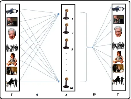
Figure 1.1: The instantaneous mixtures source separation example

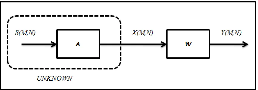
In Figure 1.1, S refers to the original sources matrix 𝑺, 𝑨is the mixing matrix and 𝑿

is the observation matrix. The matrices 𝑺 and 𝑿 are both of size𝑀 ×𝑁 matrices while

the matrix 𝑨 is of size 𝑀×𝑀. The values M and N are the number of sensors and the number of samples, respectively. The matrix 𝑺 has the form:

𝑺 =�s11⋮ ⋯⋱ s1𝑁⋮

s𝑀1 ⋯ s𝑀𝑁

(18)

1 . I n t r o d u c t i o n

3

The observation matrix X can be modeled as Follows:

𝑿 = 𝑨𝑺 (1.2) or

𝑿

=

�

𝒙

𝟏

𝒙

𝟐

.

𝒙

𝑴

�

=

�

𝑥

11

⋮

⋯ 𝑥

⋱

1𝑁

⋮

𝑥

𝑀1

⋯ 𝑥

𝑀𝑁

�

=

�

𝑎

11

⋮

⋯ 𝑎

⋱

1𝑀

⋮

𝑎

𝑀1

⋯ 𝑎

𝑀𝑀

� �

𝑠

11

⋮

⋯ 𝑠

⋱

1𝑁

⋮

𝑠

𝑀1

⋯ 𝑠

𝑀𝑁

�

(1.3)

The coefficients of the mixing matrix A are unknown. The goal of the BSS algorithms is

to find a demixing matrix W that has the following form:

𝒀 = 𝑾𝑿 (1.4) where W is an 𝑀×𝑀 matrix, Y and X are 𝑀×𝑁 matrices. The obtained estimated

sources Y using BSS algorithms have certain unknown factors such as arbitrary scaling,

permutation, and delay of estimated source signals. However, the most relevant

information is contained in the waveforms of these signals, thus these unknown factors

do not affect the separation if statistical methods like BSS are used [7]. Historically,

principle component analysis (PCA) has been widely used for the same types of problems

currently being investigated using BSS algorithms [3, 8]. The main difference between

the two approaches is that BSS finds non-Gaussian and independent sources signals,

whereas PCA finds sources, which are uncorrelated and have Gaussian distributions [3].

The performance of BSS algorithms such as FastICA is better in comparison with

the PCA [5] because PCA does not work on super-Gaussian or sub-Gaussian distributions

while FastICA does [6]. Since BSS does not require any prior knowledge about the

mixed signals, BSS has attracted many areas of research. For example, in surveillance

application where the goal is to find a specific voice among many [9, 10]. In addition,

(19)

1 . I n t r o d u c t i o n

4

multi-antenna system without requiring the receiving end to decode the signals [11]. The

most useful application in utilizing the BSS techniques would be in the area of

biomedical signal processing, where BSS is applied in Electrocardiography (ECG). Some

of the applications involve the separation of the Mother ECG (MECG) from the fetal

ECG (FECG) [12, 13]. In addition, some complex scenarios involve separating the

MECG from a twin fetal [14]. Recently, Field programmable gate array (FPGA)

technology has been the choice of implementation in the area of digital signal processing

and neural networks. Kim et al. [15] implemented real-time blind source separation and adaptive noise cancellation for speech enhancement in FPGA. Du and Qi [16]

implemented a parallel ICA on the Multi FPGA pilchard, a reconfigurable computing

development environment dedicated for Sun Microsystems [18]. Celik et al. [17] implemented a mixed-signal real-time blind source separation that can only unmix two

independent sources. The design in [17] is implemented using 0.5µm COMS technology.

Kuo-kai et al [19] implemented full real-time FPGA based FastICA system and used extra circuitry to acquire the signals using two sensors. Two separate modules were used.

The first module was used to acquire the mixed signals using an analogue to digital

converter and filters. The second module converted the separated signals to analogue

using an digital to analogue converter.

All the previously proposed FPGA implementation focused on implementing ICA

algorithms with the assumption that only two signals are mixed and only two sensors are

used to capture the mixed signals for separations. In addition, the previous work

implemented the blind source separation algorithm using algebraic solutions. For higher

(20)

1 . I n t r o d u c t i o n

5

addition, it can result in a very large propagation delay and, in turn, affects the overall

system performance.

1.2 FPGA background

FPGA is a large-scale integrated circuit that can be programmed after it is manufactured

rather than being limited to a predetermined unchangeable hardware function. FPGA

technology is widely used in digital signal processing [20]. It combines the speed of

dedicated blocks, application-optimized hardware and reprogrammability of

microprocessors, which makes it suitable for high speed implementation of blind source

separation. FPGA has been the choice of implementation of most of digital signal

processing algorithms. DSP algorithms can be designed, tested and implemented on an

FPGA chip without any fabrication delays. FPGAs consist of the following elements:

1. Programmable logic cells which provide the functional elements for construction

of the user’s input.

2. Input output (IO) Blocks which provide the interface between the logic cells and the

output pins.

3. Programmable interconnects which provide the routing paths to connect the input

and output of logic cells and the IO pins.

Modern FPGAs provide high-level arithmetic and control structures, such as

multipliers, counters, multiply accumulate units, memory resources and processor cores.

These resources provide high performance, low power consumption and are highly

suitable for DSP applications [21]. The behavior of an FPGA can be defined by using a

hardware description language (HDL) such as VHDL or Verilog or by arranging blocks

(21)

1 . I n t r o d u c t i o n

6

synthesized using proprietary FPGA place-and-route tools. The compilation and synthesis

process generates a bit file that can be downloaded on the FPGA [21, 22].

Although FPGAs are similar to custom Application-specific integrated circuit

(ASIC) design, FPGAs can implement and test proposed designs instead of sending them

to the manufacturer and wait for the chip to be tested afterwards.

1.3 Thesis objective

The thesis focuses on the following areas:

1. Investigating different types of independent component analysis (ICA) algorithms

for non-Gaussian signals and compare the results with principle component analysis

(PCA).

2. Developing an efficient numerical solution instead of the algebraic solution for

FastICA.

3. Investigating the development of FastICA algorithm using different types of

orthogonalization techniques.

4. Implementing FastICA algorithm in XILINX virtex5-XC5VLX50t FPGA.

The main challenge in this thesis is implementing the ICA algorithm for higher

order data inputs. The complexity of the circuit grows exponentially depending on the

size of the demixing matrix W. In addition, FPGA is used to implement the algorithm.

1.4 Thesis organization

This thesis is organized as follows: Chapter 2 provides the mathematical analysis of the

ICA algorithm, which is FastICA. Chapter 3 describes the proposed FastICA model using

QR method and the symmetrical orthogonalization as well as the hardware

(22)

1 . I n t r o d u c t i o n

7

simulations of the proposed hardware and presents two experiments while Chapter 5

(23)

8

Independent Component Analysis

Chapter 2

2.1 Introduction

This Chapter provides the mathematical theory behind ICA method. ICA is one of a

family of techniques, including PCA and blind deconvolution, for solving the BSS

problems. ICA is a method for finding underlying factors in a multidimensional data.

This Chapter also explains the PCA method and its limitations. Finally, a special ICA

algorithm called FastICA is presented and compared with the PCA method.

2.2 General statistical settings

The main goal of any statistical model is to find a suitable representation of the

parameters of a multivariable system that render the essential structure governing the

variables more visible. This usually presents computational and representational obstacles

that must be tackled.

To illustrate the above, a linear system is shown in Fig. 2.1. In the system, every input

vector in 𝑿 contains a linear combination of observed sensor samples of size N as in Equation (1.4) given in Chapter 1. In the figure, 𝑾is the demixing matrix of size 𝑀×𝑀.

The aim, as explained in Chapter 1, is to determine the output matrix 𝒀. However, the

system contains unknown sources with no prior knowledge of the noise type and its

(24)

2 . I n d e p e n d e n t C o m p o n e n t A n a l y s i s

9 Moreover, the difficulty of this model lies in the fact that it requires determining the

elements of the 𝑾 matrix using linear algebra, which finds a simple solution to 𝑾 only

by assuming the signals independence [23].

Figure 2.1: Linear instantaneous BSS problem

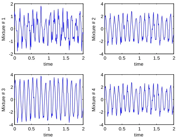
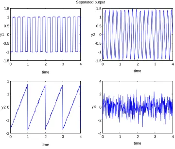
Fig. 2.2 shows four source signals that result in the mixture shown in Fig. 2.3 when

mixed together. The problem is that the original signals information is not usually

available. In fact, it is nearly impossible to know what these signals might contain when

they are mixed. But with the aid of BSS techniques, it is possible to extract or at least

estimate the hidden signals. For example, considering matrices 𝑾 and 𝑿of sizes 4 × 4

and 4 ×𝑁, respectively, using statistical independence only, the original signals in Fig.

2.2 can be estimated by multiplying 𝑾 by 𝑿 as follows:

𝒀=� 𝒚𝟏 𝒚𝟐 𝒚𝟑 𝒚𝟒 �=� 𝑤11 𝑤21 𝑤31 𝑤41 𝑤12 𝑤22 𝑤32 𝑤42 𝑤13 𝑤23 𝑤33 𝑤43 𝑤14 𝑤24 𝑤34 𝑤44 � � 𝑥11 𝑥21 𝑥31 𝑥41 𝑥12 𝑥22 𝑥32 𝑥42 𝑥13 𝑥23 𝑥33 𝑥43 ⋯ … ⋯ … 𝑥1𝑁 𝑥2𝑁 𝑥3𝑁 𝑥4𝑁

� (2.1)

As a result, Y contains four vectors that are the separated signals which are the

(25)

10 distinct signals that are not dependent of the other. The separated signals are easily

distinguished as square, sin, sawtooth, and random noise waves.

Figure 2.2: Sources before mixing

Figure 2.3: Mixed Signals that contain some underlying hidden factors

0 0.5 1 1.5 2 -2

-1 0 1 2

0 0.5 1 1.5 2 -4

-2 0 2 4

0 0.5 1 1.5 2 -4

-2 0 2 4

0 0.5 1 1.5 2 -2

-1 0 1 2

Source # 1 Source # 2

Source # 3 time

Source # 4 time

time time

0 0.5 1 1.5 2

-2 -1 0 1 2 time M ix tur

e # 1

0 0.5 1 1.5 2

e # 2

0 0.5 1 1.5 2

e # 3

0 0.5 1 1.5 2

(26)

11 Figure 2.4: Separated Signals

2.3 Principle component analysis (PCA)

PCA has been widely used in pattern recognition and signal processing [24]. The

algorithm decomposes a set of mixed signals into a set of uncorrelated signals [7]. Given

a set of multivariate measurements, the purpose of the PCA is to find a smaller set of

variables with less redundancy that would result in a good representation of the data.

PCA can classify signals based on the mixture statistical information (variances.). Each

principle component (PC) represents a cluster of information in the mixture. The PC that

has the highest variance is referred as the major component while those components with

the smallest variances called the minor components [25]. If the PCs contain high

statistical information (high variances), it means that those PCs contains real signals and

0 1 2 3 4

-1.5 -1 -0.5 0 0.5 1 1.5

0 1 2 3 4

-1.5 -1 -0.5 0 0.5 1 1.5

0 1 2 3 4

-2 -1 0 1 2

0 1 2 3 4

(27)

12 if the PCs contain very low variances, it is an indication that the mixture contains

unwanted signals like noise or interference [25].

2.3.1 PCA algorithm

PCA transforms a process such that the data are represented along a new set of

orthogonal dimensions with a diagonal covariance matrix [24]. In addition, the PC

coefficient with the largest variance is the first principle component; the PC coefficient

with the second largest variance is the second most important and so on. The PCA

algorithm consists of the following steps [24]:

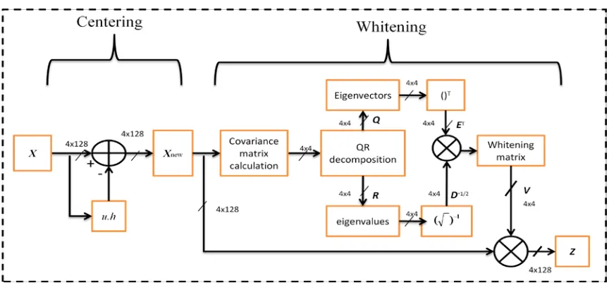
1. Centering: Centering is used as a preprocessing in PCA. Centering is the process of

calculating the mean of the observation matrix 𝑿 and subtracting it from the source. It

can be defined as:

𝑿𝒄𝒆𝒏 =𝑿 − 𝒖𝒉 (2.2)

where 𝑿_𝒄𝒆𝒏is the centered observation matrix and has the same dimension as 𝑿. The

1 ×𝑁h vector of all 1s, i.e.,

𝒉[𝑛] = 1 for 𝑛= 1, … ,𝑁 (2.3)

Moreover, u is an 𝑀× 1 vector which is the empirical mean of X and can be calculated

as:

𝑢[𝑚] = 1

𝑁∑𝑁𝑛=1𝑿(𝑚,𝑛) for 𝑚= 1, … ,𝑀 (2.4)

2. Calculating Covariance matrix and its eigenvalues and eigenvectors: The PCA

algorithm is based on calculating the eigenvalues and eigenvectors of the 𝑀×𝑀

covariance matrix 𝑪_𝒙 which isdefined as [25].

(28)

13 where E[∙] is the expectation operation. The covariance matrix is used to compute the

eigenvectors. Each eigenvector corresponds to a specific eigenvalue. Since the covariance

matrix is real and symmetric, the eigenvectors are real and orthonormal [26].

Traditionally, the eigenvalues of a matrix is calculated algebraically using the following

steps [16], [19]:

a) Find the characteristic equation of 𝑪_𝒙 by setting det(𝑪_𝒙− 𝜆_𝑚𝑰) = 0 of the

covariance matrix where I is an identity matrix that has the same dimensions as𝑪_𝒙

and𝜆_𝑚 are the eigenvalues to be found.

b) Find the roots of the characteristic equation which are the eigenvalues of𝑪_x.

The complexity of finding the roots of the characteristic equation increases when

the order of 𝑪_𝒙increase. Most of the previous separation models using PCA

approach use only 2 × 2 matrices [27, 28], which result in second order

polynomials [25]. For higher order matrices, an iterative numerical solution is used

[29]. The most common numerical methods used to find the eigenvalues and

eigenvectors for higher order matrices are the upper triangular matrix, the power

method, the orthogonal iteration, the QR decomposition and the singular value

decomposition [29, 30].

4. Whitening: which is the last stage in the PCA technique, it forces the sources in the

mixture to be uncorrelated but with a unit variance [25]. The whitening matrix V can be

expressed in terms of the eigenvalues and eigenvectors of 𝑪_x as follows [25]:

𝑽= 𝑫−𝟏/𝟐𝑬𝑻 (2.6) where E is an 𝑀×𝑀 matrix containing all the eigenvectors of 𝑪_𝒙 , while 𝑫 is an 𝑀×𝑀

(29)

14 matrix 𝑽 is also called the square root of the covariance matrix, i.e. 𝑪_𝒙−1 2⁄ [34].

The last step in the PCA is to find the uncorrelated signals 𝒁 using the following

equation:

𝒁= 𝑽𝑿_𝒄𝒆𝒏 (2.7) where 𝒁 and 𝑿_𝒄𝒆𝒏 are𝑀×𝑁matrices. In general, 𝑽 solves half of the ICA problem

which means forcing the signals to be uncorrelated and transforms the signals

orthogonally [31]. In most applications, this is not sufficient to ensure that the signals are

independent, which is why whitening solves only half of the ICA problem. However, the

whitening step reduces the computations of separation by half [34]. More specifically, the

orthogonal nature of 𝑽 reduces the problem from finding 𝑘2 parameters which are the

elements of 𝑽 to finding only 𝑘 (𝑘 −1)/2 parameters [32].

2.3.2 Whitening limitations

Assume that the data in the ICA model is whitened using Equation (2.7). The whitening

matrix transforms the mixing matrix A in equation (1.2) into a new mixing matrix called

À=𝑽𝑨 so that the new ICA model is written as follows:

𝒁 =𝑽𝑿= 𝑽𝑨𝑺 (2.8) Unfortunately, whitening cannot solve the ICA problem, since whiteness or

uncorrelatedness does not imply independence [28]. Uncorrelatedness is weaker than

independence, and is not by itself sufficient to estimate any ICA model [32].

On the other hand, whitening is useful as a preprocessing step in ICA. The usefulness of

whitening resides in the fact that the new mixing matrix Àis orthogonal [28, 33]. This

means that we can restrict the search in the mixing matrix to the space of orthogonal

(30)

15 original matrix A [7], we only need to estimate an orthogonal mixing matrix À. Thus, it

could be said that whitening solves half of the ICA problem because whitening is a very

simple and standard procedure, much simpler than any ICA algorithms. The remaining

half of ICA can be estimated by some other methods like FastICA [34], which is the

focus of this thesis. However, PCA can be used as a preprocessing step before the ICA

algorithms [31].

2.4 Higher order statistics

Most of the standard methods in signal processing systems utilize system’s statistical

information in linear discrete-time system. Although their theory is well defined and

developed [35-38], these methods are utilizing the second order statistics and are driven

by the assumptions of the source signals being stationary and are jointly governed by a

Gaussian linear underlying system. Recently, an interest in the higher order statistics has

began to grow in the signal processing area. At the same time, neural network has grown

popular with the development of several new, efficient learning algorithms [32, 23, 39].

Neural networks consist of computational blocks called neurons. The output of the

neurons depends nonlinearly on the input [40]. An example of the nonlinearity is the

hyperbolic tangent tanh(𝑼), the matrix 𝑼 is of size 𝑀×𝑁 which is the inner product

𝑼=𝑾𝑿. It introduces nonlinearity to the process [40]. ICA requires the use of higher order statistics via nonlinearities [33, 40]. In the following, the concept of kurtosis and its

role in the higher orders statistics [33].

2.4.1 Central moments and kurtosis The mean of the data vector 𝒛 is defined as:

(31)

16 where 𝒛 is a vector in the whitened data matrix 𝒁. In addition, the 𝑗𝑡ℎ central moment is

defined as:

𝑢_𝑗 =𝐸{(𝒛 − 𝑢)𝑗} (2.10)

The second central moment is the standard deviation of the whitened data Z denoted as

𝜎2_{. The third central moment is called skewness and it will be used in this thesis.}

However, the fourth moment has been intensively used in the area of blind source

separation [32, 35, 39]. Moments that are higher than 4th order are rarely used in practice

[32] and will not be discussed in the thesis.

The fourth moment on the other hand, is simple and effective in some BSS algorithm like

FastICA. The fourth central moment is [32]:

𝑢₄ =𝐸[(𝒛 − 𝑢)4] (2.11)

The fourth central moment is also called the Kurtosis and can be rewritten as [33].

𝐾𝑢𝑟𝑡(𝒛) =𝐸[𝒛4−3[𝐸[𝒛2]]2 (2.12)

We can also rewrite it in the following form [31]:

𝐾𝑢𝑟𝑡(𝒛) = 𝐸[𝒛4]

𝐸[𝒛2_]2−3 (2.13)

For whitened data 𝐸[𝒛2] = 1, the Kurtosis is reduced to the following [38]:

𝐾𝑢𝑟𝑡(𝒛) =𝐸[𝒛4]−3 (2.14)

This implies that for the whitened data, the fourth order moment can be used instead of

the Kurtosis to represent the fourth order central moment of 𝒁. The most important

property of the kurtosis is that it has the ability to detect non-Gaussian signals. If the

kurtosis is zero, it implies that the distribution is Gaussian. If the Kurtosis is negative, the

(32)

17 However, the absolute value of the Kurtosis is used for simplicity since it is only needed

to know if the signal is non-Gaussian or not [33, 38, 39, 40].

2.4.2 Fixed-point FastICA algorithm using kurtosis

In the previous section, the Kurtosis has been introduced as a measure of non-Gaussianity

[32]. The advantage of such technique can be adapted by neural networks [36]. However,

the convergence is slow and the choice of the input sequence has to be chosen carefully

[40]. A bad choice of the input sequence would lead to divergence. Alternatively, the

fixed-point iterative algorithm that has been developed by Hyvarinen and Oja is used

[39]. To achieve a more efficient fixed-point iteration, the gradient must point to the

direction of the weight vector 𝒘_𝒎= [𝑤₁,𝑤₂, … ,𝑤_𝑀]𝑇. The gradient must equal to 𝒘_𝒎

multiplied by some value. As a result, the weight vector 𝒘_𝒎 can be written as [39]:

𝒘_𝒎= [𝐸{𝒁(𝒘_𝒎𝑻𝒁)3}−3‖𝒘_𝒎‖2𝒘_𝒎] (2.15)

Equation (2.15) is further simplified as a fixed-point iteration algorithm by computing the

right hand side and assign the new value to 𝒘_𝒎. Thus Equation (2.15) can be rewritten as

follows [39]:

𝒘_𝒎← 𝐸{𝒁(𝒘𝑻_𝒎𝒁)3}−3𝒘_𝒎 (2.16)

𝒘_𝒎← 𝒘_m⁄‖𝒘_m‖ (2.17) The weight vector 𝒘_𝒎 is divided by its norm using Equation (2.17) after every

iteration in the FastICA, is a necessary normalization step to keep the variance of the

term 𝒘_𝑚𝑇𝒁 constant [33]. If the PCA is considered as a preprocessing stage prior to the

FastICA, the FastICA algorithm would have the following steps:

1. Center the input 𝑿.

(33)

18 3. Choose 𝑀 the number of independent components to be estimated.

4. Initialize the first vector w to any random numbers.

5. Run the FastICA algorithm on 𝒘.

6. Normalize 𝒘 by dividing it by its norm.

7. If 𝒘 has not converged, go back to step 3.

where w is a vector in 𝑾= [𝒘_𝟏,𝒘_𝟐,𝒘_𝟑, … ,𝒘_𝑴]𝑻 . However, it can be noticed that the

algorithm searches for a single weight vector in 𝑾 which means only one signal can be

estimated. That is why this method is called one-unit FastICA [32]. To estimate the other

weight vectors 𝒘_𝑀, anorthogonalization step is needed after the search has converged to

the first weight vector 𝒘_𝟏 [40]. Otherwise, the search might converge to the same

maxima [34] if other initial values were to be applied in step 2. Actually, this iterative

technique has a very fast convergence and reliable [30]. The algorithm has two main

superior advantages over the normal gradient-based algorithms. Firstly, the convergence

of this algorithm is cubic. It implies that the convergence is rapid [31]. Secondly, this

algorithm has no learning rate or other adjustable parameters [32].

2.5 FastICA usingorthogonalization techniques

So far, the search algorithm that has been discussed finds one component in the mixture.

In most of time, 𝑿 has more than one component, that is why it is necessary to account

for the other components in the weight matrix 𝑾. Also, the search algorithms don’t

usually converge to orthogonal results as in theory [32], which is why orthogonalization

must be applied at every step in FastICA [41]. The key concept of orthogonalization is

(34)

19 subspace. The most common techniques are the Gram-Schmidt or sometimes called

deflationary orthogonalization method and the symmetric orthogonalization [32].

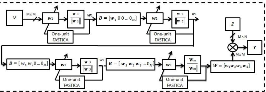
2.5.1 FastICA usingdeflationary orthogonalization

Deflationary orthogonalization is simple and the oldest technique in orthogonalization

[41]. It estimates the independent components one by one using Gram-Schmidt method.

Followed by running the one-unit FastICA for 𝒘_𝑚 where m is the number of independent components 𝑚 = 1, . . ,𝑀 . After every iteration, projections (𝒘_𝑚+1𝑇 𝒘_𝒊)𝒘_𝒊 where

𝑖= 1, … ,𝑀 of the previously estimated m vectors is subtracted from 𝒘_𝑚+1 [31]. After the first successful calculation, the values of the first weight vector 𝒘₁ are obtained.

Similarly, after the mth iteration , the values of the corresponding vector 𝒘m are obtained.

The resulting values of all the vectors obtained from the iterations are placed in the final

unmixing matrix 𝑾 of size 𝑀×𝑀.

It is worth noting that for simplicity purposes, an intermediate matrix 𝑩 is used by

the algorithm to hold the values of the generated 𝒘m as they are obtained in the

corresponding iteration. When the final iteration is complete, the final separation matrix

𝑾 is equivalent to 𝑩.

The final output matrix 𝒀 is then obtained by multiplying 𝑾 by the whitened data matrix

𝒁[32, 34, 42, 43].

The deflationary orthogonalization can be added to the one-unit FastICA so that the

algorithm can separate M independent components using the following steps [30]: 1. Center the input 𝑿 so that it has zero mean.

2. Whiten the 𝑿_𝑐𝑒𝑛 matrix to give 𝒁.

(35)

20 4. Initialize the vector 𝒘_𝑚 to any random numbers.

5. Initiate the FastICA algorithm on 𝒘_𝑚.

6. If 𝒘_𝑚 has not converged, go back to step 3.

7. Start the deflationary orthogonalization using the following Equation:

𝒘_𝒎← 𝒘_𝑚− ∑𝑚−1_𝑗=1 �𝒘_𝑚𝑇𝒘_𝑗�𝒘_𝑗 (2.18)

8. Normalize 𝒘_𝑚 by dividing it by its norm.

𝒘_𝑚 =𝒘_𝑚⁄‖𝒘_𝑚‖ (2.19)

9. Setm←m+1. If m is not greater than the desired number of IC, go back to step 2.

The norm in step 7 is the second norm [32]. The Deflationary orthogonalization is

shown in Fig. 2.5. It is clear that the process is serial, which indicates that the weight

vectors 𝒘_𝑀 are calculated sequentially.

Figure 2.5: Deflationary orthogonalization block diagram

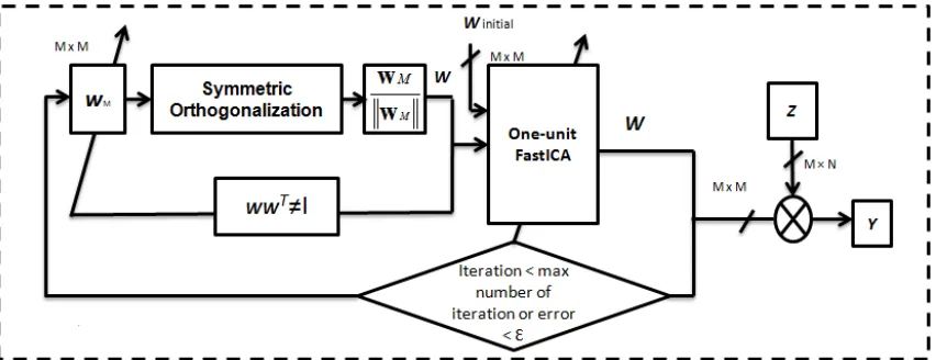
2.5.2 FastICA usingsymmetric orthogonalization

In some cases, sequential orthogonalization like the deflationary approach is not suitable

for implementation [28]. Symmetric orthogonalization on the other hand finds the

orthogonal vectors 𝒘_𝑚 that are the vectors of 𝑾 in parallel. Symmetric orthogonalization

(36)

21 by orthogonalizing 𝑾 using symmetrical method. The symmetrical orthogonalization is

performed using the following equation [30, 32, 36]:

𝑾 ←(𝑾𝑾𝑇)−1 2⁄ 𝑾 (2.20) In other words the FastICA steps using the symmetrical orthogonalization can be

described as:

1. Center the input 𝑿 so that it has zero mean.

2. Whiten the 𝑿_cen matrix to give 𝒁.

3. Choose 𝑀, the number of Independent components to be estimated. (Set 𝑚 = 1).

4. Initialize the vector 𝒘_𝑚 𝑚 = 1, … ,𝑀 to any random numbers.

5. Initiate the FastICA algorithm on every 𝒘_𝑚in parallel.

6. Perform a symmetric orthogonalization of the matrix 𝑾= [𝒘_𝟏, … ,𝒘_𝒎]𝑇 using

Equation (2.20).

7. Normalize 𝑾 by dividing it by its norm.

8. If 𝑾 has not converged, go back to step 3.

The inverse square root (𝑾𝑾𝑻)−1 2⁄ is obtained from the eigenvalue decomposition of

(𝑾𝑾𝑻_{) =}_𝑬_{𝑑𝑖𝑎𝑔}₍_𝑑

1, … ,𝑑𝑚) 𝑬𝑇[29], where E is an 𝑀×𝑀 matrix that contains the

eigenvectors of (𝑾𝑾𝑻) and �𝑑₁−1 2⁄ , … ,𝑑_𝑚−1 2⁄ � are the eigenvalues of (𝑾𝑾𝑻). The

eigenvalue decomposition can be further expanded as [38]:

(𝑾𝑾𝑻)−1 2⁄ = 𝑬𝑑𝑖𝑎𝑔�𝑑1−1 2

⁄ _{, … ,}_𝑑

𝑚−1 2⁄ �𝑬𝑇 (2.21)

Fig. 2.6 shows FastICA algorithm using symmetrical orthogonalization. The

algorithm starts by initializing 𝑾_{𝑖𝑛𝑖𝑡𝑖𝑎𝑙} to some random values. The orthogonalization is

performed after every iteration in the FastICA. The FastICA algorithm is monitored by

(37)

22 Figure 2.6: FastICA algorithm using Symmetric Orthogonalization

Notwithstanding, this method has some practical limitation due to the complexity of

the matrix inversion calculation [30], especially when the order of W is high. An

alternative iterative approach reported in [30, 32, 38] is used to solve this issue and is

described by:

1. 𝑾= 𝑾 ‖𝑾‖⁄ (2.22)

2. 𝑾= 3

2𝑾 − 1

2𝑾𝑾𝑇𝑾 (2.23)

3. If 𝑾𝑾𝑻 is not close enough to the identity matrix go back step 2.

The technique starts with a non-orthogonal matrix 𝑾. The iterations continue until

𝑾𝑾T_~_𝑰_{is achieved. The convergence of the method is proven in Appendix}_A_.

The advantage of this technique relies on the fact that matrix inversion is

computationally intensive and calculating Equation (2.20) in every loop in the FastICA

renders the hardware slow and inefficient [39]. Instead, Equations (2.22) and (2.23) are

used to replace Equation (2.20). The norm in Equation (2.22) can be any norm, but for

simplicity the second norm is used which is the maximum summation of the largest

(38)

23

2.6 Summary

In this chapter, the PCA and ICA models have been explained. Independent component

analysis (ICA) is a method for finding underlying factors or components from

multivariate (multidimensional) statistical data. What distinguishes ICA from other

methods is that it looks for components that are both statistically independent and

non-Gaussian where the PCA just decorelates the signals based on their variances. This

chapter also explained the FastICA algorithm and how to use orthogonalization

techniques to find all components of 𝑾. In addition, deflationary and symmetrical

(39)

24

Chapter 3 Proposed Architecture and FPGA Implementation

3.1 Introduction

Having presented the PCA and FastICA algorithms in Chapter 2, I now detail the

implementation process of the FastICA using PCA as a preprocessing stage. In Section

3.2, the proposed model is explained, after which the realization of the eigenvalues and

eigenvectors is given in Section 3.3. The FastICA orthogonalization process is explained in

Section 3.4. Section 3.5 gives the details of the hardware implementation while Section 3.6

presents the final implementation of the algorithm. The chapter ends with a summary in section

3.7.

3.2 Proposed model

The proposed BSS model accepts up to four input sensors. This assumption is interrupted

as the model can separate up to four mixed signals in the mixture. The sources in the

mixture are assumed to be independent and non-Gaussian. Let 𝒀describes the separated

signals in Equation (2.1) with the model being expanded to account for 4 signals. The

number of samples is set to 𝑁 = 128. The components of 𝒀 are estimated by multiplying

the 4 × 4 unmixing matrix 𝑾 by the 4 × 128 input matrix 𝑿. It is noted that the input

signals are also assumed to be independent and non-Gaussian.

𝒀 =𝑾𝑿= � 𝑤11 𝑤21 𝑤31 𝑤41 𝑤12 𝑤22 𝑤32 𝑤42 𝑤13 𝑤23 𝑤33 𝑤43 𝑤14 𝑤24 𝑤34 𝑤44 � � 𝑥11 𝑥21 𝑥31 𝑥41 𝑥12 𝑥22 𝑥32 𝑥42 𝑥13 𝑥23 𝑥33 𝑥43 ⋯ … ⋯ … 𝑥1,128 𝑥2,128 𝑥3,128 𝑥4,128

(40)

3 . P r o p o s e d A r c h i t e c t u r e a n d F P G A I m p l e m e n t a t i o n

25

Equation (3.1) shows the mathematical model used in the separation of the mixed signals.

The goal of the ICA algorithm is to estimate the unmixing matrix 𝑾. To do so, the PCA

algorithm is first applied to force the signals to be uncorrelated and then the FastICA

algorithm is applied. However, calculating the whitening matrix is not straightforward

since the 𝑪_𝑥 have the same dimension as 𝑾, i.e.

𝑪𝒙 = � 𝑐11 𝑐21 𝑐31 𝑐41 𝑐12 𝑐22 𝑐32 𝑐42 𝑐13 𝑐23 𝑐33 𝑐43 𝑐14 𝑐24 𝑐34 𝑐44

� (3.2)

Finding the eigenvalues and eigenvectors algebraically for large covariance

matrices such as Equation (3.2) is not computationally efficient. Instead, numerical

solution is used in implementation [28]. However, only few iterative techniques can

converge to find all the eigenvalues of the required matrices. For example, the power

method finds only the dominant eigenvalue. Moreover, the convergence of the power

method is the eigenvalues convergence is too slow and is not suitable for implementation

[28]. The only simple and robust numerical solution that can find all eigenvalues and

eigenvectors is the QR decomposition method [43]. However, the method works only on

symmetric and positive definite matrix, fortunately, the 𝑪_𝒙 have these two properties [44,

45].

Since the covariance matrix is symmetrical, the only elements in the covariance

matrix that are not repeated are the diagonal elements. Hence, the covariance matrix can

be put in the form:

𝑪_𝒙 = � 𝑐11 𝑐01 𝑐02 𝑐03 𝑐01 𝑐11 𝑐12 𝑐13 𝑐02 𝑐12 𝑐33 𝑐23 𝑐03 𝑐13 𝑐23 𝑐33

(41)

26

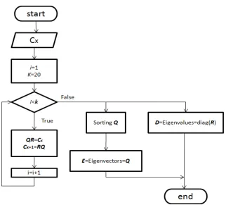
3.3 Realization of eigenvalues and eigenvectors

In this thesis, the QR decomposition is used to find the eigenvalues and eigenvectors

numerically instead of finding them algebraically. Figure 3.1 shows the flow chart that

describes the QR decomposition method [26].

The value K is the number of the maximum iterations. There is no specific value for K, however, QR decomposition can achieve good result if the value of K is more than 10 [26]. Nevertheless, in this work, it is decided to set 𝐾= 20 so that the result of the QR

decomposition is approximately close to 3-significant figures. The matrices 𝑹 and 𝑸 that

result from the method are both of size 𝑀×𝑀. High-precision approximation is required

because the hardware implementation is carried out using fixed-point number system and

the error that builds in the calculation may affect the result of the QR decomposition

method.

(42)

27

According to Fig. 3.1, the eigenvalues are obtained by taking the diagonal elements

of the 𝑹 matrix. However, the eigenvectors require more steps to get the final 𝑬matrix.

The output of the flowchart given in Fig. 3.1 is two matrices𝑫and 𝑬 representing

the eigenvalues and eigenvectors respectively. Their role is to obtain the whitening

matrix 𝑽 as given in Equation (3.4) given as follow:

𝑽=𝑫−𝟏/𝟐_𝑬𝑻 ₌_�

𝑑1−1 2⁄

0 0 0

0 𝑑2−1 2⁄

0 0

0 0 𝑑3−1 2⁄

0

0 0 0 𝑑4−1 2⁄

� � 𝑒11 𝑒21 𝑒31 𝑒41 𝑒12 𝑒22 𝑒32 𝑒42 𝑒13 𝑒23 𝑒33 𝑒43 𝑒14 𝑒24 𝑒34 𝑒44 � 𝑇 (3.4)

In the equation, for each eigenvector of matrix 𝑬 (e.g. [𝑒₁₁𝑒₁₂ 𝑒₁₃ 𝑒₁₄]𝑇) is

represented by a column denoting the corresponding eigenvalue in matrix

𝑫 ([𝑑₁−1 2⁄ 0 0 0]𝑇_).

The uncorrelated output 𝒁 is obtained by multiplying the whitening matrix 𝑽

obtained from Equation (3.4) by 𝑿_𝒄𝒆𝒏. Fig. 3.2 shows the complete centering and

whitening process using the QR decomposition.

(43)

28

3.4 FastICA using symmetric orthogonalization

This thesis focuses on implementing the FastICA algorithm by utilizing symmetric

orthogonalization. This modification entails that the final unmixing matrix 𝑾 (shown in

Fig. 2.6 of Chapter 2) is 4 × 4 as given in Equation (3.1).

To begin with, finding the symmetric orthogonalization of the unmixing matrix 𝑾

((𝑾𝑾𝑇)−1 2⁄ 𝑾 given in Equation (2.20) requires calculating the term (𝑾𝑾𝑇)−1 2⁄ . A

standard algebraic method is to multiply the eigenvalues and eigenvectors 𝑬 and 𝑫 of the

term (𝑾𝑾𝑇) [31]. The problem is that for higher-order matrices (such as the 4 ×

4 unmixing matrix𝑾 of this work), calculating the eigenvalues and eigenvectors 𝑬 and

𝑫 (both 4 × 4) is computationally-intensive [32]. What complicates the matter further is

that this calculation must be performed iteratively in every step of the FastICA algorithm

given in Chapter 2.

Alternative approaches have been proposed. One such approach is to use an

iterative model to speed up the process of symmetrical orthogonalization. This approach

was introduced in Chapter 2, Equations (2.22) and (2.23). Indeed, the iterative method

converges to the same solution provided by the more expensive algerbraic method after

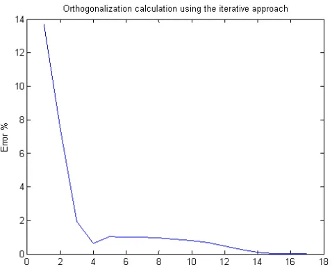
less than 20 iterations as the simulation I performed given in Fig. 3.3 shows. The

simulation given in the figure is separates the sources using the iterative method. The

x-axis represents the number of iterations required for convergence while the y-x-axis

represents the error between the current result of the iterative approach and the final

result given by the algebraic approach. The simulation ends when the two solutions

match giving zero error.

(44)

29

because we are only modeling the number of iterations and not the time required to reach

a solution. In fact, the 15 iterations performed by the iterative method converge to a

solution much faster than the computations performed algebraically. This is a known

property of iterative methods [34].

Figure 3.3: Symmetrical orthogonalization simulation using iterative approaches

3.5 FPGA implementation

It is well-known that the FPGA implementation of the FastICA algorithm is carried out

using XILINX virtex5-XC5VLX50t FPGA chip. The LX50t chip has superior speed and

larger area over the other virtex5 family [46]. The design is implemented using VHDL

language. Since the system is designed to account for higher order data (four sensors),

hierarchy is adopted throughout the design to provide a better control over the overall

hardware structure and to monitor the overflow and underflow of each block.

Furthermore, implementation of DSP systems using floating-point arithmetic

requires a huge hardware area and may lead to inefficient design especially for FPGA

implementation [18]. On the other hand, fixed-point representation results in efficient

(45)

30

consists of an integer part and a fractional part as shown in Fig. 3.4.

Figure 3.4: Fixed-point representation

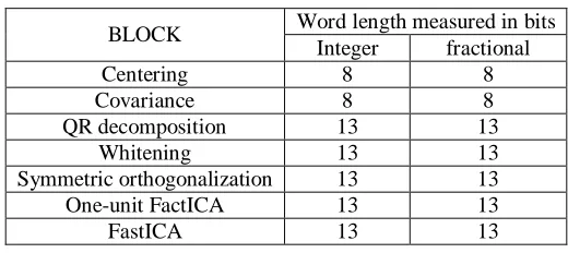
The word length was selected based on several simulation attempts. Most of the

results were faulty when a small word length was used since the small word length was

not sufficient to represent the values. After several simulations attempts, the choice of the

word length was decided not to be the same for various implementation blocks. For

example, the QR decomposition block, the I/O and the intermediate signals word lengths

were set to (26:13) which indicates 26 bits with 13 bits representing the integer part and

13 bits representing the fractional bits. This way, the integer part can represent numbers

in the range of 213 = 8192. For the Centering and Covariance blocks, the word length

was set to 16 bits because the calculation of the Centering and the Covariance were not

complex and 16 bits were enough to represent for the intermediate variables like signals

and storage elements within the implementation blocks. In general, the word lengths of

(46)

31

Table 3.1: Blocks word length used.

BLOCK Word length measured in bits Integer fractional

Centering 8 8

Covariance 8 8

QR decomposition 13 13

Whitening 13 13

Symmetric orthogonalization 13 13

One-unit FactICA 13 13

FastICA 13 13

3.6 Hardware implementation

This Section describes the implementation stages of the complete system. The main block

is divided into two stages namely Whitening and FastICA as shown in Fig. 3.5. Both

stages have no control over each other. However, when the first stage, i.e. the whitening

stage finishes its operation and the result is ready, the second stage is triggered by the

main controller in Fig. 3.5. The main controller starts the process of the entire design; it

enables and disables each block in the design based on the order of operation.

The controller consists of a finite state machine (FSM). The GO_FASTICA and

GO_whitening signals are used to enable both stages in the design. In addition,

CLK_whitening and CLK_FASTICA are the clocks supplied to Whitening and FastICA

blocks. Address_sel_mem1 and CLK_mem1 are used for an intermediate RAM that

holds the result of the Whitening stage and feed it to the FastICA block when required.

Different clocks are used to reduce the power consumption and to provide a better control

over the design. First, the controller activates the Whitening block to preprocess the

signals and when the process is complete, the Whitening_busy signal becomes low

allowing the controller to activate the FastICA. However, in order to pipeline the design,

the Whitening block stays on after the process is complete to process another packet of

(47)

32

New_one control signal activates the whole process again when the FastICA finishes

processing the first packet, the signal FastICA_Busy goes low when the first packet is

processed by the FastICA to indicate that FastICA is ready to take another block of data

from the Whitening block. Each packet contains 26 × 128 × 4 bits of data stored in a

ROM. Nevertheless, for the sake of simulation, only one packet of 128 samples is used in

testing the implementation.

(48)

33

Table 3.2: Complete system FPGA resources utilization report.

Information Count Percentage Use

Slice Registers 27779 of 28800 96%

Slice LUTs 28403 of 28800 99%

Slice LUTs used as Logic 28584 of 28800 99% Slice LUTs used as RAM 413

LUT Flip Flop pairs used 27674

LUT Flip Flop pairs with an unused Flip Flop 10689 of 27674 39% LUT Flip Flop pairs with an unused LUT 5432 of 27674 20% Fully used LUT-FF pairs 11553 of 27674 41%

Unique control sets 326

IOs 240

Bonded IOBs 240 of 360 67%

BUFG/BUFGCTRLs 26 of 32 81%

Block RAM/FIFO 51 of 60 85%

DSP48Es 45 of 48 94%

Table 3.3: Complete system performance report.

Clock

name Frequency response MAX operating frequency Estimated period

Input sampling

CLK 20.0 MHz 16.2 MHz 62.5 ns 1.857

KSPS

Table 3.2 shows the complete system FPGA resources utilization report. In can be

noticed that the system has been fully synthesized on a single FPGA chip since the area

of implementation is still less than 28800 registers which is the available Slice registers in

virtex5-XC5VLX50t. The total number of I/O pins used is 240 pins out of 360. Table 3.3

shows the maximum operating clock which is measured as 16.2 MHz when the system

CLK is 20 MHz. The following sections describe the details of implementation of the

algorithm.

3.6.1 Implementation of whitening

The Whitening block contains three stages namely, Centering, Covariance, and QR

(49)

34

Figure 3.6: Whitening block

The first stage is the Centering block where the data is first fetched from the

memory and the expected values are calculated and subtracted from the 𝑿 according to

Equation (2.2). The second stage calculates the covariance matrix of the centered signals

while the third stage calculates the eigenvalues and eigenvectors of the covariance

matrix. The MAIN CONTROLLER activates the Whitening block first. The Whitening

implementation block is shown in Fig. 3.7. There are 128 samples fetched to the

centering block for processing. RAM block 1 is activated to store 𝑿_𝑐𝑒𝑛 after the data is

centered. R_w1 and R_w2 are the controller’s read and write operations in both RAM

Modules. RAM Module 2 is in read mode as the Whitening result is available and the

whiten_busy signal goes low. Multiplier 2 whitens the data by multiplying the 𝑽 by 𝑿_𝑐𝑒𝑛.

RAM Module 2 keeps the whitened results for further analysis by other blocks. In

addition, the data in RAM Module 2 will be available until another packet of information

(50)

35

Figure 3.7: Whitening implementation block

Table 3.4 shows the resources utilization of the Whitening block when implemented

separately. The overall area utilization is about 25% of the overall FPGA chip area. In

addition, Table 3.5 indicates the Whitening maximum frequency, which is measured as

63 MHz when the block is simulated using the input CLK_Whitening set to 50 MHz .

Table 3.6 is an extension of Table 3.5. It shows the timing details of CLK_Whitening

through the Whitening clock.

Table 3.4: Whitening FPGA resources utilization report.

Information Count Percentage

Use

Slice Registers 7407 of 28800

25%

Slice LUTs 8382 of

28800 29%

Slice LUTs used as Logic 8202 of

28800 28%

Slice LUTs used as RAM 180 LUT Flip Flop pairs used 10834 LUT Flip Flop pairs with an unused Flip

Flop

3427 of

10834 31%

(51)

36 10834

Fully used LUT-FF pairs 4955 of

10834 45%

IOs 240

BUFG/BUFGCTRLs 1 of 32 3%

DSP48Es 27 of 48 56%

Table 3.5: Whitening performance report.

Clock name Input frequency MAX operating

frequency

Estimated period

Input sampling

CLK_Whitening 50.0 MHz 62.189 MHz 16.08 ns 6.857 KSPS

Table 3.6: Whitening timing report.

Clock name Path name Estimated

Frequency Estimated period

CLK_Whitening Input to Register 135.2 MHz 7.3964 ns

CLK_Whitening Register to

Register (worst case) 62.189 MHz 16.08 ns CLK_Whitening Register to Output 265.4 MHz 3.7679 ns

It is worth noting that there is an apparent discrepancy between the input frequency

in Tables 3.3 and 3.5. In order to explain this, I draw attention to the fact that for blocks

varying in complexity, the maximum frequency that can be assigned to the block will

vary. This is because each block can take a certain frequency after which the simulation

will not be correct due to internal delays.

For example, in Table 3.3, the input frequency assigned to the complete system has

to be low to account for all the blocks in the design to avoid timing problems. This is

because if a higher frequency is used, the intermediate blocks will not produce the correct

results in time for the following blocks to process the data. Using the same logic, a higher

(52)

37

therefore permit such increase. In the rest of this section, different input frequencies will

be set to accommodate the design complexity accordingly.

3.6.1.1 Implementation of Centering block

The centering stage is the first sub block of the whitening operation. Centering means

removing the mean of each input vector (128 samples) by subtracting the mean values

from the original signals. The Centering stage contains 16-bit adders, 16-bit dividers and

16-bit subtractors. The mean of the four signals are calculated simultaneously since the

signals are loaded at the same time to the Centering block as shown in Fig. 3.8. Table 3.7

also shows the mean gate-level results in comparison with the simulated MATLAB.

According to Table 3.7, the results from the MATLAB simulation is considered very

close to the gate-level simulation.

Figure 3.8: Implementation of centering

In addition, the accuracy of the Centering block can be increased by increasing the

(53)

38

implementation process, 16 bits is considered adequate for all signals in the Centering

block given in Fig. 3.8.

Table 3.7: Mean calculations result.

The Centering Controller enables the three blocks in series using FSM. After the adder’s

result is available, a 16-bit divider is used to compute the mean of the four results over

128 samples according to Equation (2.4). Moreover, the ROM that holds the input

requires 128 cycles to load the 128 input samples to the Centering block. In addition, the

adder, the divider and the subtractor require 3 clock cycles to complete their task.

According to the simulation results, the Centering output is available after 131 clock

cycles. Table 3.8 shows the Centering FPGA resources utilization report. Table 3.9 shows

the maximum frequency when the input the CLK_cen frequency is 100 MHz. It is measured

as 150.7 MHz, in other words, this block cannot accept more than 150 MHz as CLK_cen.

Table 3.10 provides more details about the CLK_cen path throughout the design.

Table 3.8: Centering FPGA resources utilization report.

Information Count Percentage Use

Slice Registers 2548 of 28800 8%

Slice LUTs 1417 of 28800 4%

Slice LUTs used as Logic 1417 of 28800 4% LUT Flip Flop pairs with an unused Flip Flop 369 of 2917 12%

LUT Flip Flop pairs with an unused LUT 1500 of 10865 51% Fully used LUT-FF pairs 1048 of 10865 35%

IOs 134

Variable name MATLAB Result Gate-level Simulation

res1 0.3488 0.3486

res2 0.2758 0.2756

res3 0.3044 0.3041

FPGA Implementation of Blind Source Separation using FastICA

Scholarship at UWindsor

Scholarship at UWindsor

FPGA Implementation of Blind Source Separation using FastICA

FPGA Implementation of Blind Source Separation using FastICA

FPGA Implementation of Blind

Source Separation using FastICA

Author’s Declaration of Originality

Abstract

Acknowledgments

Table of Contents

List of Figures

List of Tables

List of Abbreviations

Chapter 1

Introduction

𝑿

=

�

𝒙

𝒙

.

𝒙

�

=

�

𝑥

⋮

⋯ 𝑥

⋱

⋮

𝑥

⋯ 𝑥

�

=

�

𝑎

⋮

⋯ 𝑎

⋱

⋮

𝑎

⋯ 𝑎

� �

𝑠

⋮

⋯ 𝑠

⋱

⋮

𝑠

⋯ 𝑠

�

Independent Component Analysis

Chapter 2

Chapter 3

Proposed Architecture and FPGA Implementation