ABSTRACT
BILLINGS, JERILYN MARIE. Evolution and Maintenance of the 2223 June 2003 Noc-turnal Convection during BAMEX. (Under the direction of Matthew D. Parker.)
On 2223 June 2003 two mesoscale convective systems (MCSs) evolved throughout the evening and night time hours and were observed by the Bow Echo and Mesoscale convective vortex Experiment (BAMEX). These two MCSs were studied by analyzing the observations, and performing both case study and idealized model simulations. The rst of these MCSs originated from a group of supercells that had been initiated in a northsouth line along a preexisting outow boundary in eastern Nebraska. These supercells anchored to the preexisting outow boundary leading to large rainfall totals and facilitating cell mergers. These cell mergers increased the depth and strength of the surface cold pool, which became the forcing mechanism for new convection. As this happened, the convection reoriented from a northsouth line of isolated supercells into an eastwest, southward propagating squall line. While the squall line was developing and reorienting, isolated supercells developed along the dryline in northcentral Kansas. These supercells moved northeastward, eventually passing the southward propagating squall line and evolving into a small MCS that continued to move northeastward during the night.
Evolution and Maintenance of the 2223 June 2003
Nocturnal Convection during BAMEX
by
JERILYN MARIE BILLINGS
A thesis submitted to the Graduate Faculty of North Carolina State University
in partial fulllment of the requirements for the Degree of
Master of Science
Marine, Earth, and Atmospheric Sciences
Raleigh, North Carolina 2007
APPROVED BY:
Matthew D. Parker, Chair of Advisory Committee
Dedication
Biography
Jerilyn Billings was born on June 6th, 1982 and grew up in Kearney, Nebraska. After a short weather section in 8th Grade Earth Science sparked her interest, she knew she wanted to become a meteorologist.
After graduating from Kearney Senior High School in 2000, she attended the Univer-sity of Nebraska at Kearney, before transferring to the UniverUniver-sity of Oklahoma to fulll her dream. While she was an undergraduate she volunteered at the National Weather Service in both Hastings, Nebraska and Norman, Oklahoma and realized that operational meteorology was what she ultimately wanted to pursue. One opportunity that was in-valuable to her, took place during the spring semester of her junior year at Oklahoma when she took part in the Study Abroad program in at the University of Reading in Reading, England where she continued to study meteorology. Jerilyn graduated with a Bachelor's of Science in Meteorology in August 2004. After taking a year o from school, she began the master's program at North Carolina State University in the Fall of 2005. Following the completion of her degree she will pursue a career in operational meteorology.
Jerilyn enjoys traveling and was blessed with the opportunity to travel throughout the United States when she was younger which instilled a love for traveling that continues to this day. Jerilyn will take trips to wherever and whenever she can. Driving, ying, or taking the train it's all an adventure and she hopes to visit all the ends of the earth. Although she had been to Europe before, after living in England for six month, her love for Europe grew and she plans on taking an extended trip following the completion of her Master's degree.
Acknowledgments
Contents
List of Figures vii
List of Tables xii
1 Introduction 1
2 Background 4
2.1 Supercell Dynamics . . . 7
2.2 Mesoscale Convective System Dynamics . . . 10
3 Data and Methods 14 3.1 Observations . . . 14
3.2 Numerical Models . . . 16
3.2.1 Case Study Simulations . . . 16
3.2.2 Idealized Simulations . . . 21
4 Observational Analysis 31 4.1 Synoptic Environment . . . 31
4.2 Background Mesoscale Environment . . . 32
4.3 Initial Supercells . . . 39
4.4 Consolidation into a Squall Line . . . 43
4.5 Subsequent Evolution . . . 47
4.5.2 Isolated Northeastward moving Nocturnal Storms . . . 53
4.5.3 Nocturnal Event . . . 60
4.6 Observational Conclusions . . . 61
5 Case Study WRF Simulations 64 5.1 Initial WRF Run . . . 64
5.2 Articial Addition . . . 76
6 Idealized Simulations 83 6.1 Simulations with Simple Forcing . . . 84
6.1.1 Warm Bubble . . . 85
6.1.2 Cold pool . . . 90
6.1.3 Simple forcing Conclusions . . . 92
6.2 Simulations with Complex forcing . . . 93
6.3 Simulations with Colliding Storms . . . 98
6.4 Articial Nocturnal Cooling . . . 104
6.4.1 Nocturnal Chilling Applied to a Warm Bubble Simulation . . . . 105
6.4.2 Nocturnal Chilling applied to the Merger Simulation . . . 111
6.5 Idealized Simulation Conclusions . . . 118
7 Concluding Remarks 119 7.1 Discussion . . . 119
7.2 Future Work . . . 122
7.3 Conclusions . . . 123
List of Figures
1.1 Base radar reectivity at 0702 UTC and 0832 UTC from KUEX. . . 3
2.1 Accumulated precipitation during the warm season. . . 5
2.2 Hovmöller diagram showing the maximum in nocturnal convection. . . . 6
2.3 Pressure and vertical vorticity perturbations that arise when an updraft interacts with environmental wind shear. . . 9
2.4 Idealized ow associated with vertical wind shear and a surface cold pool. 11 3.1 National Weather Service sites and radar locations. . . 15
3.2 Comparison of surface temperatures between observations and case study model simulations. . . 18
3.3 Outer and inner model domains for case study simulations. . . 19
3.4 Potential temperature at 925 hPa showing articial warm bubble. . . 21
3.5 SkewT lnp plots for dropsondes 16, 17, and 18. . . 22
3.6 Dropsonde locations with respect to the convective line at 0623 UTC. . . 23
3.7 Observed 0000 UTC sounding from Topeka, KS and the point sounding from the case study simulation. . . 24
3.8 The initial temperature perturbations for the simple forcing idealized model simulations. . . 26
3.10 Initial temperature perturbation for the idealized merger model
simula-tion. . . 29
4.1 Synoptic environment on 1200 UTC 22 June 2003. . . 33
4.2 Synoptic environment on 0000 UTC 23 June 2003. . . 34
4.3 Synoptic environment on 1200 UTC 23 June 2003. . . 35
4.4 Surface boundaries valid at 2200 UTC 22 June 2003. . . 36
4.5 Base reectivity of the morning storms over eastern Nebraska. . . 37
4.6 0000 UTC 23 June 2003 skewT lnp plots and hodographs for Topeka, KS and Omaha, NE. . . 38
4.7 Base radar reectivity and radial velocity at 0003 UTC 23 June 2003. . 40
4.8 Vertical cross section through the storms at 0003 UTC. . . 41
4.9 Storm tracks through the event for the storms of interest. . . 42
4.10 Base radar reectivity at 0033 UTC 23 June 2003 and RHI cross section. 44 4.11 Base scan radar reectivity and radial velocity at 0208 UTC 23 June 2003. 46 4.12 Vertical cross section through the storms at 0208 UTC. . . 47
4.13 Base radar reectivity and radial velocity at 0332 UTC 23 June 2003. . 48
4.14 Vertical cross section through the storms at 0332 UTC. . . 49
4.15 Surface temperatures at 0600 UTC showing the cold pool under the squall line. . . 50
4.16 Base radar reectivity and the location of ASOS and Dropsondes. . . 51
4.17 SkewT lnp plots for dropsondes 11 and 17. . . 52
4.18 Base scan and cross section of radial velocity at 0959 UTC 23 June 2003. 54 4.19 Base radar reectivity from KDDC at 0153 UTC 23 June . . . 55
4.20 Base radar reectivity of the northeastward moving storms. . . 56
4.21 Radial velocity at 2.4◦showing the mesocyclone in supercell I. . . . 57
4.22 Base radar reectivity and radial velocity at 0702 UTC from KUEX. . . 58
4.24 Hodographs of dropsondes 15, 16, 17 and 18. . . 61 4.25 Base radar reectivity and radial velocity at 0832 UTC from KUEX. . . 62 4.26 Vertical cross section through the storms at 0832 UTC. . . 63
5.1 Comparison of observations and the case study simulation at 1800 UTC 22 June. . . 65 5.2 Simulated reectivity at 2110 UTC in case study simulation. . . 67 5.3 Cold pool of squall line in the case study simulation at 0050 UTC 23 June
2003. . . 68 5.4 SkewT lnp plots from south and west of the cold pool at the surface at
0050 UTC. . . 69 5.5 The presence of a moist absolutely unstable layer (MAUL) ahead of the
convective line. . . 70 5.6 Simulated reectivity of squall line at 0200 UTC. . . 71 5.7 SkewT lnp diagram ahead of the squall line at 0700 UTC 23 June. . . 72 5.8 Simulated reectivity at 925 hPa of the squall line. . . 73 5.9 Cross section through the squall line at 0700 UTC. . . 74 5.10 Parcel trajectories launched ahead of the squall line in the case study
simulation. . . 75 5.11 Maximal heights of 400 parcels launched in the lowest 500 m AGL between
0630 and 0730 UTC. . . 76 5.12 SkewT lnp diagrams comparing the observed location of the supercells
and the location where the articial warm bubbles were placed. . . 77 5.13 Simulated reectivity of supercell at 0210 UTC 23 June 2003 in case study
simulation. . . 78 5.14 Simulated reectivity of the squall line and supercell at 0210 UTC 23 June
5.16 Cross section through the supercell showing vertical vorticity and pertur-bation pressure at 0210 UTC. . . 81 5.17 Parcel trajectories from the updraft of the supercell in the case study
simulation. . . 82
6.1 Simulated reectivity and vertical vorticity showing rotating updrafts at 35 min. . . 86 6.2 Cross section through the updraft showing vertical velocity and the
pres-sure perturbation. . . 87 6.3 Simulated reectivity and the cold pool at the surface at 1 hr in the warm
bubble simulation. . . 88 6.4 Simulated reectivity and the cold pool at the surface at 3 hours. . . 88 6.5 Vertical cross sections through the rightmoving supercell and the center
of the squall line. . . 89 6.6 Vertical cross section through the cold pool, in the cold pool forcing
sim-ulation. . . 91 6.7 Simulated reectivity and the cold pool at the surface in the cold pool
simulation. . . 92 6.8 Comparison of the "complex" model setup and the observed environment. 94 6.9 Simulated reectivity and the cold pool of the complex simulation at 1
hour. . . 95 6.10 Simulated reectivity and the cold pool of the complex simulation at 2
hours. . . 95 6.11 Evolution of the complex simulation at 3.5 hours showing simulated
re-ectivity and the cold pool. . . 96 6.12 Simulated reectivity and the cold pool at the surface showing storm D is
6.14 Simulated reectivity and the cold pool at the surface in the Merger sim-ulation at 1 hour. . . 99 6.15 Simulated reectivity showing storm mergers and new storm F. . . 100 6.16 Simulated reectivity and cold pool 10 minutes after the merger. . . 101 6.17 Time series of column averaged values for the area surrounding the merger. 102 6.18 Rainfall dierence between hours 2 and 3 following the cell mergers. . . 103 6.19 Simulated reectivity showing propagation of the eastern half of the squall
line. . . 104 6.20 Comparison of the cold pool's at the surface in the simulations with and
without chilling. . . 107 6.21 Cross sections through the cold pools in the simulations with and without
chilling. . . 108 6.22 Lifting due to the vertical pressure gradient force in the nocturnal warm
bubble simulation. . . 110 6.23 Cross section of buoyancy and vertical pressure gradient force. . . 111 6.24 Parcel trajectories entering the updrafts in the nocturnal warm bubble
simulation. . . 112 6.25 Comparison of the simulated reectivity of the squall line in the
List of Tables
3.1 Physics options used in the case study WRF simulations. . . 20 3.2 Initial model setup for idealized model runs. . . 25
Chapter 1
Introduction
Mesoscale convective systems (MCSs), dened as a contiguous area of precipitation that is at least 100 km in one direction, are extremely common in the midlatitudes, and account for a large percentage of the warm season precipitation in these regions of North America (Fritsch et al. 1986). While this precipitation is benecial to agriculture and key to the growing season, MCSs are often associated with localized ooding and severe weather as well, having a detrimental impact on society. It has also been shown in previous studies that a nocturnal maximum in organized convection exists over the central Great Plains (Carbone et al. 2002). The high societal impact of MCSs implies a need for accurate forecasts of MCS events. However, forecasting nocturnal convection is dicult because the mechanisms that sustain these convective systems are poorly understood (McNulty 1995). Many nocturnal convective events are believed to be elevated, feeding on air above the stable nocturnal layer. Elevated convective systems are less likely to produce severe winds and tornadoes, thus it is important to know whether nocturnal systems are elevated or surfacebased. Surfacebased convection is dened for this study as convection that ingests air from the surface layer (below 500 m)1. However, without a continual means of sampling the entire lower troposphere it is dicult to determine in real time whether MCSs are elevated or not. Numerical models often produce inaccurate
forecasts of convective mode and motion, likely due to incorrect representation of physical processes such as cloud microphysics (Fritsch and Carbone 2004). Therefore, in order for operational forecasts to improve, our understanding of physical processes must be advanced, especially when it comes to nocturnal convection. With this in mind, a key question to be answered is: what mechanism is responsible for lifting air parcels to their level of free convection in elevated and surfacebased nocturnal MCSs?
0702 UTC
L
M
(a) 0702 UTC
0832UTC
L
M
(b) 0832 UTC
Figure 1.1: Base scans of radar reectivity (dBZ) at (a) 0702 UTC and (b) 0832 UTC 23 June 2003 from KUEX.
remain surfacebased within a seemingly similar, stable, nocturnal environment.
Chapter 2
Background
MCSs have been widely discussed in the literature, including many signicant papers about their organization, evolution and propagation. Much of the knowledge base was reviewed in two very detailed summary papers by Fritsch and Forbes (2001) and Houze (2004) . MCSs have a region of deep moist convection that is at least 100 km long in one direction (Houze et al. 1990, 2004), often with an associated stratiform precipitation area. Common severe weather threats from MCSs include ooding, strong winds, large hail, and weak tornadoes. Fritsch et al. (1986) quantied the eect that MCSs have on the agriculturally dependent central Great Plains, concluding that MCSs account for a large fraction (30% to 70%) of the precipitation that falls during the warm season (AprilSeptember) (Fig. 2.1).
Figure 2.1: Accumulated precipitation (cm) from 44 MCC's from the 1982 warm season taken from Fritsch et al. (1986). Hatched and shaded regions indicate precipitation accumulations of 1 to 5 cm and ≥20 cm, respectively.
During the summer of 2003 a eld program was conducted over the Great Plains and Midwest to further study MCSs. The Bow Echo and MCV Experiment (BAMEX; Davis et al. 2004) focused on the dynamics of bow echoes (Weisman 1993, 2001) and mesoscale convective vortices (MCVs; Menard and Fritsch 1989; Cotton et al. 1989; Houze 2004), both of which are commonly associated with MCSs. Many studies of bow echoes and MCVs have been undertaken using the copious data from BAMEX. However, one event during BAMEX was memorable for its intense supercells that eventually evolved into a squall line during the evening and overnight hours on 2223 June 2003. Two of the initial supercells were very strong; the Aurora, Nebraska supercell (Guyer and Ewald 2004) which produced the largest hailstone on record (Knight and Knight 2005), and the Superior, Nebraska supercell, (Wakimoto et al. 2004) which had the highest measured wind speeds ever recorded in a mesocyclone. While these two phenomena are interesting and important to understand, the focus of the current research is the complex evolution of the supercells into a squall line, the additional supercells that evolve into an MCS and the subsequent propagation of these two MCS. In contrast to MCSs, supercells are smaller, strong, isolated storms which carry a high potential for producing large hail, strong damaging winds and violent tornadoes. The dynamics of both supercells and MCSs were important in this case, and will be reviewed in turn.
2.1 Supercell Dynamics
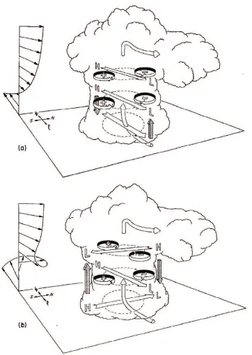
cycloni-cally/anticyclonically rotating cells after they split (Rotunno and Klemp 1982, 1985; Klemp 1987). In a clockwise/counterclockwise turning vertical wind shear prole the right/left moving cell is sustained by a dynamically induced vertical pressure gradient force (Fig. 2.3; Rotunno and Klemp 1982, 1985; Weisman and Klemp 1984; Klemp 1987). Weisman and Klemp (1984) concluded that these dynamic eects account for 60% of the updraft strength, with buoyancy accounting for the remaining 40%. Weis-man and Rotunno (2000) found that both linear (the "preferred right/left mover eect") and nonlinear (the "storm splitting eect") eects are important and impact the prop-agation of a supercell, but they found that the nonlinear eects give the best overall explanation of supercell propagation. In either case, the relevance to the present study is that supercells can dynamically lift environmental air even when its buoyancy is small (or even negative).
There are additional studies in the literature that discuss the initiation and evolution of supercells. In an idealized study, Bluestein and Weisman (2000) found that the orien-tation of the vertical wind shear vector with respect to a line of cells was important in determining whether individual cells merged together or remained isolated. In their sim-ulations, right/left moving supercells from the interior of the line often merged with the adjacent left/right moving cell while supercells on the ends of a line remained longlived and isolated. Supercells located on the end of a line are likely to remain isolated and longlived due to the reduced chance of interactions with other supercells and/or their cold outow boundaries.
(1994). Many studies have found that merging cells often have enhanced precipitation production, possibly due to reduced entrainment of dry air and increased precipitation eciency due to the large volume of hydrometers among the merged cells. In addition to the enhanced precipitation production it has also been suggested in the literature that cell mergers can be precursors to tornadogenesis (Lemon 1976; Finley et al. 2001; Lee et al. 2006). In observational studies by Lemon (1976) and Finley et al. (2001) and numerical studies by Kulie and Lin (1998) updraft strength and midlevel rotation increased after a cellmerger. In the present case, supercell mergers over time led to a large, intense MCS. The dynamics relevant to the MCSs phase are reviewed next.
2.2 Mesoscale Convective System Dynamics
The summary paper by Fritsch and Forbes (2001) discusses two dierent types of MCSs that are identied based on their dierent dynamical forcing mechanisms. "Type 1" MCSs occur as a result of potentially unstable air being forced upward at a frontal zone or other baroclinic boundary. In other words, the ascent is a consequence of synoptic scale features. "Type 2" events rely upon systemscale cold pool forcing; the ascent is maintained by features developed by the convection itself. Many nocturnal MCSs we presume to be "type 1" systems, driven by the moisture uxes and upglide associated with the lowlevel jet. Such systems are decoupled from the nocturnal or postfrontal boundary layer and hence are "elevated". The storms present on 23 June developed along a preexisting cold outow boundary in Nebraska and transitioned into a squall line. The analysis in chapters 4 6 strongly suggest that this squall line was surfacebased and cold pooldriven. In other words, it was of the "type 2" variety. Hence, we review here literature that is relevant to "type 2" (cold pooldriven) squall lines.
Figure 2.4: Idealized ow associated with vertical wind shear and a surface cold pool, taken from Weisman and Rotunno (2004). Left: cold pool spreads away from a decaying convective cell in an environment with no vertical wind shear. Right: lowlevel vertical wind shear balances coldpool circulation on the downshear side, enhancing the ability to regenerate convective cells through deeper lifting.
squall lines, now known as RKW theory (named for the authors Rotunno, Klemp, and Weisman). RKW theory posits that vertical wind shear can maintain a squall line by favoring the development of new convection on the downshear side of a surface cold pool, where the environmental wind shear opposes the circulation associated with the cold pool (Fig. 2.4). Rotunno et al. (1988) and Weisman and Rotunno (2004) provide evidence that an "optimal" state can be achieved for a squall line when moderate to strong shear is conned in the lowest 22.5km above ground level. Numerous other studies have since shown that the cold pool and wind shear play a large role in the organization of a squall line. Robe and Emanuel (2001) also found in their study that linear convective systems tend to reorient themselves such that their orientation becomes perpendicular to the lowlevel shear.
of Mexico. This moisture transport and isentropic lift by the nocturnal LLJ appears to be one of the most important factors for the initiation, maintenance and propagation of nocturnal convection over the Great Plains (Blackadar 1957; Astling et al. 1985; Colman 1990a,b; Trier and Parsons 1993; Trier et al. 2006). Nocturnal convection, especially that associated with the LLJ, is often thought to be elevated convection; in other words, it is thought to be maintained by feeding on air parcels located above the boundary layer. Observational studies by Colman (1990a, 1990b), Rochette and Moore (1996), and Moore et al. (2003), among others, have documented that the majority of elevated convective systems are initiated north (on the cold side) of a surface front. The surface front, coupled with warm, moist advection and the secondary circulations associated with the LLJ provide ascent along and north of the boundary, where conditional or potential instability can be realized (Rochette and Moore 1996; Moore et al. 2003). In the present case the convective event was not on the cold side of a front; the isolated thunderstorms began as surfacebased storms during the late evening hours, and then the atmospheric boundary layer slowly cooled nocturnally, bringing into question whether these storms remained surfacebased, or transitioned into an elevated system during the night.
cooled throughout the night, meaning that it may be an example of a nocturnal convective system that is actually surfacebased.
Chapter 3
Data and Methods
3.1 Observations
BAMEX was an observational eld program based at MidAmerica St. Louis Airport near St. Louis, Missouri. The objective of BAMEX was to use mobile platforms to gain unprecedented highdensity kinematic and thermodynamic observations within and near MCSs in order to study bow echoes and MCVs. The mobile platforms included two P3 aircraft. A Learjet from Weather Modication Inc (WMI) deployed dropsondes from 12 km above ground level (AGL) (Davis et al., 2004).
KLBF
KOAX
KUEX
KTOP
KDDC
Figure 3.1: The National Weather Service sites and radar sites used in this study: Hast-ings, NE (KUEX), Omaha, NE (KOAX), North Platte, NE (KLBF), Topeka, Kansas (KTOP), and Dodge City (KDDC). Radar reectivity at 0623 UTC 23 June 2003 to show locations of radars with respect to the storms.
Weather Service (NWS) sites were analyzed, including Hastings, Nebraska (UEX), Om-aha, Nebraska (OAX), North Platte, Nebraska (LBF), Topeka, Kansas (TOP), Dodge City, Kansas (DDC), and Goodland, Kansas (GLD) (Fig. 3.1).
June 2003. In addition to the surface data, upper air data at the mandatory levels (925 hPa, 850 hPa, 700 hPa, 500 hPa, 300 hPa, and 250 hPa) were also analyzed using the NARR data in order to depict the synoptic environment of the event.
Dropsonde data from the BAMEX eld catalog were plotted, and then multiple thermodynamic and kinematic variables, including convective available potential energy (CAPE), convective inhibition (CIN), lifted condensation level (LCL), level of free convec-tion (LFC), equilibrium level (EL) and equivalent potential temperature were computed. The thermodynamic parameters were calculated for three dierent parcels, the surface based parcel (SB), the most unstable parcel (MU), and a parcel with mean values from a 1 km mixed layer (ML). Hodographs were also created and analyzed using the wind values from the dropsondes and other soundings. Additionally, operational NWS sound-ings from the OAX, LBF, TOP sites were also used to depict the vertical prole of the prestorm environment near the MCSs.
3.2 Numerical Models
Case study and idealized model simulations were conducted to supplement the de-tailed observational analysis. The 2223 June 2003 MCSs were simulated with real data using the Advanced Research (ARW) core of the Weather Research and Forecasting (WRF) Model . In order to isolate and strip down the dynamics and processes occurring during the event, idealized simulations were also produced using the Bryan Cloud Model 1 (CM1, Bryan and Fritsch 2002).
3.2.1 Case Study Simulations
The WRFARW is a fully compressible nonhydrostatic model. Atmospheric elds were integrated using the 3rd order RungeKutta time scheme, 5th order horizontal ad-vection and 3rd order vertical adad-vection. Case study simulations were initialized using the 32 km gridded North American Regional Reanalysis (NARR) data (Mesinger et al., 2006) in the WRF standard initialization (WRFSI) preprocessing software. The simula-tions were initialized at 1800 UTC on 22 June 2003 and integrated for eighteen hours. The NARR data were also used to update the domain's lateral boundary conditions every three hours.
During the time period in which this research was conducted, a new version of WRF was released, version 2.2. In order to test the robustness of the results, new simulations were performed using version 2.2. However, these simulations did not perform as well as those run with version 2.1.1. One main dierence between version 2.1.1 and version 2.2 was the preprocessing system, with version 2.1.1 using the WRF standard initialization and version 2.2 using the WRF preprocessing system. The same input NARR data were interpolated onto the model grid with an initial time of 1800 UTC 22 June 2003, but the initial elds in the version 2.2 simulation were radically dierent from both those in the simulation using version 2.1.1, and the objectively analyzed observations (Fig. 3.2a,b,c). While some of the model variables in version 2.2 had magnitudes that were closer to those observed, their placement and overall shapes were dierent. The positions of the observed outow boundary, stationary front, and dry line were very important for the subsequent initiation and location of the storms that developed; and the positions of these features in version 2.1.1 were much closer to those observed. The surface values in version 2.2 also had very unusual and unrealistic jumps. Due to these dierences, and the fact that it produced a simulation that was a closer representation to what was observed, version 2.1.1 was used for the "production simulations" in this research.
(a) Version 2.1.1 (b) Version 2.2
Observed surface temperature (F) at 1800 UTC 22 June 2003
(c) observed surface temperature
Figure 3.2: Comparison of temperature (◦F, contoured) at the rst model level at 1800
d02
d01
Figure 3.3: Outer(d01) and inner(d02) model domains used in the case study simulations.
approximately 760 km by 760 km in size with a horizontal grid spacing of 1.33 km in the x and y directions, was used to better represent the convection over Nebraska and Kansas (Fig. 3.3). While a horizontal grid spacing of 1.33 km does not exactly repli-cate the small scale circulations associated with squall lines, horizontal grid spacing on the order of 1 km does reproduce basic squall line circulations as discussed by Weisman et al. (1997) and Bryan et al. (2003). The computational expense of high resolution simulations dictated, to a certain degree, the horizontal grid spacing for the simulations. Both the inner and outer domains had 31 stretched vertical levels with the top level at 100 hPa. The 100 hPa model top is a restriction due to the use of the NARR data for the initialization and lateral boundary conditions. The average vertical grid spacing was approximately 520 m, ranging from ∼81 m in the lowest level of the domain to ∼1000 m
Table 3.1: The physics options used for the case study WRF simulations
Process Longwave
Radiation
Shortwave Radiation
Surface Layer Land Surface
Model Planetary Boundary Layer Paramet-erization Rapid Radiative Transfer Model (RRTM) Dudhia Monin-Obukhov Six layer Rapid Update cycle (RUC) Yonsei University (YSU)
parameterization was not used. Water and phase change processes were controlled using a six class water microphysics scheme as developed by Lin et al. (1983) on both the inner nested and outer model domains. The additional physics options used for the simulations are included in table 3.1.
Figure 3.4: Potential temperature (K, shaded) at 925 hPa at 0130 UTC from the case study simulation. Warm bubble is outlined by the black circle above.
discussed in detail in Chapter 5.
3.2.2 Idealized Simulations
The Cloud Model Version 1 (CM1), release 11 was used to conduct the idealized model simulations. CM1 was developed by George Bryan and Michael Fritsch at The Pennsylvania State University (PSU) and is supported by George Bryan. The model's dynamical framework is described by Bryan and Fritsch (2002) and is designed primarily for idealized research.
dierenc-(a) Dropsonde 16 (b) Dropsonde 17 (c) Dropsonde 18
Figure 3.5: SkewT lnp plots for dropsondes used as a base state sounding for idealized model runs. (a) Dropsonde 16 from 0626 UTC, (b) dropsonde 17 from 0634 UTC, and (c) dropsonde 18 from 0640 UTC. All dropsondes were launched during BAMEX on the 23 June 2003. Dropsonde locations are shown in Fig. 3.6.
ing scheme, 6th order horizontal advection and 5th order vertical advection schemes. To reduce small scale numerical noise, 6th order monotonic horizontal and vertical diusion were also present in the model. The model domain size varied with the dierent idealized simulations, but the horizontal grid spacing of 1 km was kept constant in both the x and y directions. The domain height was 20 km for all of the idealized simulations; however, the vertical grid was stretched to allow for better resolution in the lowest layers of the model. The average grid spacing in the vertical was 350 m, ranging from 200 m in the lowest level of the domain to 500 m above 3 km. All of the lateral boundaries were openradiative to allow gravity waves to propagate o of the domain. For each test a selected external sounding was used for the base state environment, and the convection was initiated using several dierent methods described below.
Drop15 Drop16 Drop17
Drop18 Drop11
Drop15 Drop16 Drop17
Figure 3.6: Dropsonde locations with respect to the convective line at 0623 UTC 23 June 2003.
(a) Topeka, KS 0000 UTC (b) Point Sounding
Figure 3.7: Soundings used as base state soundings in the idealized simulations. (a) 0000 UTC Topeka, KS sounding, and (b) a point sounding, from−98.5 W longitude and 40.21 N latitude at 0128 UTC in the case study simulation.
of 2223 June was observed to develop.
Convection was initiated in the idealized domain using various warm bubble and cold pool congurations (Table 3.2). In the rst variation, a gaussian shaped warm bubble was inserted. The warm bubble was centered 1.5 km above the ground, with a 10 km horizontal radius, a 1.5 km vertical radius and was 3 K warmer than the environment at its center (Fig. 3.8a,b). The second method to initialize convection was a cold pool; a dome of cold air with a constant potential temperature perturbation. The cold pool was 8 K colder than the environment at its center, was centered at the ground and had a horizontal radius of 50 km and a depth of 3 km (Fig. 3.8c,d).
Table 3.2: Initial model set up for idealized model runs. This table includes four model congurations: the rst, a single warm bubble (see Fig. 3.8a,b), second, a single cold pool (see Fig. 3.8c,d), the third is a complex setup with a quarter circle cold pool (CP) and 4 warm bubbles (WB) (see Fig. 3.9), and the nal model setup, the merger setup, with a quarter circle cold pool (CP) and 5 warm bubbles (WB) (see Fig. 3.10).
Model Run Name Initial Sounding Domain Size (km)
Perturbation Horizontal (H) and
Vertical (V) Radii of perturbations
Warm Bubble 16, 17, 18,
TOP, PS
400 x 400 3 K H: 10 km
V: 1.5 km
Cold Pool 16, 17, 18,
TOP, PS
400 x 400 −5 K H: 50 km
V: 1.5 km
Complex PS 400 x 600
Two dierent model setup's:
1. −2 K (CP)
and 3 K (WB)
2. −5 K (CP)
and 3 K (WB)
Initial cold pool:
H: 300 x 300 km
V: 1.5 km
Warm Bubbles:
H: 10 x 10 km
V: 1.5 km
Merger PS 400 x 600
Two dierent model setup's:
1. −2 K (CP)
and 3 K (WB)
2. −5 K (CP)
and 3 K (WB)
Initial cold pool:
H: 300 x 300 km
V: 1.5 km
Warm Bubbles:
H: 10 x 10 km
(a) Warm bubble perturbation (b) Cross section through warm bubble
(c) Cold pool perturbation (d) Cross section through cold pool
cold pool initial perturbation, the overwhelming tendency was for new convection to form on the downshear side of the initial perturbation. Rotunno et al. (1988) and Weisman and Rotunno (2004) describe this eect, often referred to as "RKW Theory". RKW theory states that the deepest lifting occurs on the side of the cold pool where the circulation associated with the vertical wind shear opposes the circulation associated with the cold pool. Because the goal of the simulation was to simulate convection similar to what was present during the 2223 June event, more complex initial perturbations were created to mimic the observed prestorm conditions and deemphasize the convection produced on the downshear side of any cold pools in the model.
A
C
B
D
Figure 3.9: Initial potential temperature perturbation (K, shaded) for the "complex" set up at 1 km AGL. One km AGL was chosen to show the locations of all features. The cold pool had a minimum temperature perturbation of−2 K at the surface and the four 3 K warm bubbles (AD) are centered at 1.5 km AGL.
a vertical radius of 1.5 km.
The "merger" model initialization setup built on the previous "complex" model setup by adding another warm bubble (E) to the domain (Fig. 3.10). The additional warm bubble was placed in the domain such that it would produce a storm that collided with the storm produced by warm bubble D during the simulation. Observations revealed that cell mergers were important in the evolution of the squall line in this case (see section 4.4, Fig. 4.10). This simulation was also run twice with two dierent cold pool temperatures,
−2 K and −5 K.
E
D A
C B
Figure 3.10: Idealized merger model domain setup with added warm bubble E. Potential temperature perturbation (K, shaded) at 1 km AGL to showing all of the features, the cold pool and warm bubbles. The cold pool had a minimum temperature perturbation of −5 K at the surface with the ve 3 K warm bubbles centered at 1.5 km AGL.
Tref = 301K−(t−3h)•n
K
h (3.1)
at each timestep after t = 1h for the nocturnal warm bubble simulation or t = 3h for the nocturnal merger simulation, with 301 K as the starting temperature at the surface. The temperature at all points below 1.5 km AGL was reset to be:
T =min(T, Tref). (3.2)
Chapter 4
Observational Analysis
During the evening hours of 22 June 2003 and the early morning hours of 23 June 2003, two MCSs were present over eastern Nebraska and northeastern Kansas. An initial northsouth oriented line of isolated thunderstorms and a few supercells evolved into two separate MCSs, covering portions of Nebraska and Kansas. However, these MCSs were two dierent modes of convection moving in dierent directions. This chapter provides an analysis of the observations.
4.1 Synoptic Environment
advected moisture northward into eastern Nebraska leading up to the event (Fig. 4.2). The nocturnal LLJ present throughout the event on the early morning hours of 23 June 2003 (Fig. 4.3) continued to provide a source of lowlevel moisture for the MCSs.
At the surface throughout the event, a high pressure system dominated the Midwest while a stationary front was draped across the central Plains (Fig. 4.1d, 4.2d, 4.3d). A dryline was present at the surface in western Kansas extending south/southwestward into the Oklahoma and Texas panhandles (Fig. 4.4). The stationary front and dryline will be discussed further in section 4.2. Twentyfour hours before the event in this study, scattered thunderstorms occurred over the central Plains on the evening of 21 June 2003 and had moved into eastern Nebraska by the early morning hours of 22 June 2003 (Fig. 4.5). This convection had a signicant impact on the mesoscale environment over eastern Nebraska and will be discussed further in the next section.
4.2 Background Mesoscale Environment
The thunderstorms from the morning of 22 June produced a stable and persistent outow boundary over the majority of eastern Nebraska, extreme northeastern Kansas into South Dakota and Iowa (Fig. 4.4). The outow boundary slowly moved westward into central Nebraska throughout the day. Solar heating warmed the surface boundary layer throughout the afternoon on 22 June 2003, however, the cool, stable outow warmed at a dierent rate. To the south and west of the outow boundary at TOP the warming destabilized the atmosphere, the convective available potential energy (CAPE) was high (3808 J kg−1), and there was essentially no convective inhibition (CIN, −0 J kg−1) (Fig.
(a) 250 hPa (b) 500 hPa
(c) 850 hPa
H
(d) Surface
Figure 4.1: Synoptic environment objectively analyzed from NARR data (chapter 3.2.1) on 1200 UTC 22 June 2003. Constant pressure plots at (a) 250 hPa with height (m, black contours, interval 12 dam), temperature (◦C, red contours, interval 5◦C) and wind
(knots, shaded, interval 25 knots above 75 and contoured at 50 knots). (b) 500 hPa with height (m, black contours, interval 6 dam), temperature (◦C, red contours, interval
5 ◦C) and wind (knots, shaded, interval 10 knots above 50 knots and contoured at 40
knots). (c) 850 hPa with height (m, black contours, interval 3 dam), temperature (◦C, d
contours, interval 5 ◦C), mixing ratio (g kg−1, green dashed contours, interval 2 g kg−1)
(a) 250 hPa (b) 500 hPa
(c) 850 hPa
H
(d) Surface
(a) 250 hPa (b) 500 hPa
(c) 850 hPa
H
(d) Surface
Outflow
Boundary
Dryli
ne
Stati
onary
Front
Remnants of morning convection
Figure 4.5: Base reectivity of the morning storms over eastern Nebraska at 1600 UTC 22 June 2003.
waves on top of the stable layer persisted throughout the afternoon (Fig. 4.4). The cold outow was approximately 5 K colder than the environment to its south and west. The Omaha, NE 0000 UTC (Fig. 4.6b) sounding characteristic of the environment within the outow layer had less CAPE (2473 J kg−1) and more CIN (−33 J kg−1) than the
environment outside the layer. The western edge of the outow boundary was roughly aligned from north to south in central Nebraska, while the southern edge was aligned almost from west to east over extreme northeastern Kansas (Fig. 4.4). This orientation of the outow boundary was key in the eventual evolution of the observed squall line.
0 -4 0 -2 0 0 2 0 4 0
LCL (hPa) 876 LF C (hPa) 875 CA PE (J /k g ) 3 80 8 CIN (J /k g ) 0
E H (0 -3 ) 3 64
S tm D ir 2 5 8 S tm S p d 2 2
(a) Topeka, KS 0000 UTC
0 -4 0 -2 0 0 2 0 4 0
LCL (hPa) 863 LF C (hPa) 7 7 0 CA PE (J /k g ) 2 64 0 CIN (J /k g ) -34
E H (0 -3) 2 4 5
S tm D ir 2 5 2 S tm S p d 2 0
(b) Omaha, NE 0000 UTC
Oklahoma panhandle and into the Texas panhandle (Fig. 4.4). Even though storms did enter the more stable environment over the Nebraska panhandle from northeast Colorado and eastern Wyoming, they did not persist in the nocturnal environment and they did not have any impact on the MCSs in the eastern part of Nebraska. With the added lift provided by the outow boundary and the moisture rich, strongly sheared, and con-ditionally unstable air to its south, the environment was prime for the development of severe thunderstorms over eastern Nebraska and northeastern Kansas.
4.3 Initial Supercells
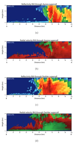
Isolated storms were initiated on the western edge of the northsouth oriented outow boundary in southcentral Nebraska around 2200 UTC 22 June 2003. Some of these storms quickly matured into supercells. Two of them, one located over the city of Aurora, Nebraska (storm A) and the other located south of it over the town of Deshler, Nebraska (Storm B, Figs. 4.7a,b) will be discussed further. Storm tracks of the labeled storms referenced below are shown in Fig. 4.9.
Ouflow Boundary Dry Line
B
A
0003 UTC
‘
A B
B’ A’
(a) radar reectivity
A
B
0003 UTC
(b) radial velocity
Reflectivity RHI through Aurora supercell
5 10 15
0
0 10 20 30 40 50 60 70 80 90 100
H e ig h t (k m )
D istance (km )
0003 U TC
A A’
(a)
Radial velocity RHI through Aurora supercell
5 10 15
0
0 10 20 30 40 50 60 70 80 90 100
H e ig h t (k m )
D istance (km ) 0003 U TC
A A’
(b)
Reflectivity RHI through Deshler supercell
5 10 15
0
0 10 20 30 40 50 60 70 80 90 100
H e ig h t (k m )
Distance (km ) 0003 U TC
B B’
(c)
Radial velocity RHI through Deshler supercell
5 10 15
0
0 10 20 30 40 50 60 70 80 90 100
H e ig h t (k m )
Distance (km ) 0003 U TC
B B’
(d)
Aurora
Superior
Deshler
KU EX
a
b
A
B
d
e
c
j
k
i
g
h
K
I
H
G
J
C
D
E
f F
N ebraska
Kansas
Storm tracks for im portant storm s
N ebraska Kansas
throughout the event.
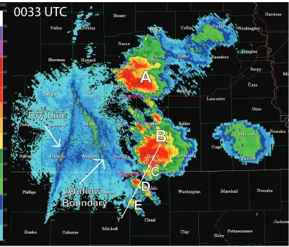
The rst couple of isolated storms that developed along the NebraskaKansas state line moved to the northeast toward Deshler, Nebraska. The northernmost storm became quasistationary along the preexisting outow boundary (storm B, Figs. 4.7, 4.8c,d, and 4.10a,b), while a storm to its southwest collided with it (storm C, Fig. 4.10). Around the same time that the Aurora supercell was dropping extremely large hailstones (0000 UTC 23 June), several tornadoes were reported near Deshler, NE. Although these severe storms were not the focus of the present study, they reected an environment that favored strong supercells. The storms also set the stage for the subsequent evolution investigated here. The Deshler storm remained quasistationary for some time, while storm mergers began to change its structure.
4.4 Consolidation into a Squall Line
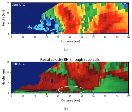
Between 2200 UTC 22 June and 0200 UTC 23 June 2003, at least six individual storms merged with the Deshler supercell. The mergers of the isolated storms into the Deshler supercell impacted its evolution and subsequent characteristics. The fourth (storm C), fth (storm D) and sixth (storm E) of these colliding storms can be seen in the 0033 UTC Hastings, Nebraska (KUEX) Doppler radar scan (Fig. 4.10). At 0033 UTC storm C had already collided with the Deshler Supercell (storm B), storm D had developed and storm E was beginning to form. By 0208 UTC, KUEX Doppler velocity data showed a large region of northerly outow winds (highlighted in Figs. 4.11b and 4.12b) indicating that the Deshler storm was no longer rotating and was predominated by lowlevel outow (Figs. 4.11a,b). The mergers cut o the updraft of the Deshler storm ultimately leading to its demise and a new dominant supercell (storm F) was able to develop to the south of the dissipating Deshler supercell, ingesting the high Θe air south of the outow boundary. A
B
A
C
D
E
Oufl
ow
Boundary
Dry
Li
ne
0033 UTC
Y
Y’
(a)
Reflectivity RHI through merging cells
5 10 15
0
0 10 20 30 40 50 60 70 80 90 100
H e ig h t (k m )
D istance (km)
0033 U TC
Y’
Y
(b)
(Fig. 4.11b), near Superior, Nebraska. The Superior supercell was also quasistationary throughout its lifetime, similar to the Deshler Supercell, anchoring to the preexisting outow boundary. In addition to the operational KUEX radar, the Superior supercell was sampled by the BAMEX airborne radars (Wakimoto et al. 2004). The Doppler velocity measurements from the airborne radars recorded the strongest mesocyclone in history (Wakimoto et al. 2004).
F
A
B
0208 UTC
(a) radar reectivity
F
A
B
0208 UTC
(b) radial velocity
5 10 15
0
0 10 20 30 40 50 60 70 80 90 100
H e ig h t (k m )
D istance (km )
0208 U TC
(a)
Radial velocity RHI through supercells
5 10 15
0
0 10 20 30 40 50 60 70 80 90 100
H e ig h t (k m )
D istance (km )
0208 U TC
(b)
Figure 4.12: Range height indicator vertical (RHI) cross sections at 0208 UTC 23 June 2003 of (a) radar reectivity and (b) radial velocity through the Deshler and Superior supercells (storms B and F) with area of interest highlighted. Color scales and location (left side of the cross section is the west end of the white line) can be found in Fig. 4.11a.
4.5 Subsequent Evolution
0332 UTC
A
F
J
I
H
(a) radar reectivity
0332 UTC
A
F
Outflow from Supercell
(b) radial velocity
Reflectivity RHI
5 10 15
0
0 10 20 30 40 50 60 70 80 90 100
H e ig h t (k m )
D istance (km )
0332 U TC
(a)
Radial velocity RHI
5 10 15
0
0 10 20 30 40 50 60 70 80 90 100
H e ig h t (k m )
D istance (km )
0332 U TC
(b)
Observed surface temperature at 0600 UTC
Figure 4.15: Objectively analyzed observed surface temperatures (◦F, blue contours) at
0600 UTC showing the cold pool (black circle) associated with the squall line.
4.5.1 Nocturnal Squall Line
The cold pool present over southeastern Nebraska and northeastern Kansas was ap-proximately 710◦F (45 K) cooler than the surrounding environment (Fig. 4.15). The
Concordia (KCNK) and Manhattan (KMHK), Kansas surface observations (locations can be found in Fig. 4.16) reveal that the squall line continued to possess a surface cold pool well into the nighttime hours. At 0455 UTC the KCNK Automated Surface Ob-serving System (ASOS) recorded a surface temperature of 27◦C with a southerly wind.
Approximately ten minutes later the temperature decreased by 7◦C and the wind became
northerly. However, at KMHK, approximately 65 miles (104 km) south of KCNK, the ob-servations remained at 26◦C with southsoutheasterly winds over the next hour. These
TWX
0502 UTC
I
F
(a) 0502 UTC
TWX
Portion of lead ing ed ge of cold p ool
0603 UTC
I
K
M
(b) 0603 UTC
(a) Dropsonde 11 (b) Dropsonde 17
Figure 4.17: SkewT lnp plots for dropsondes released into and near the convection on 23 June 2003 (a) dropsonde 11 released at 0546 UTC and (b) dropsonde 17 released at 0634 UTC. Locations are shown in Fig. 3.6.
In addition to the surface observations, numerous dropsondes were launched in and around the MCSs during the nighttime hours, providing valuable assessments of the environment in front of and within the cold pool. Dropsonde 11 was released at 0546 UTC (Fig. 4.17a) behind the convective squall line in the environment containing the cold pool (Figs. 3.6 and 4.16). This environment was very stable with small surface based CAPE (536 J kg−1) and large surface based CIN (−467 J kg−1), characteristic of an MCS
cold pool. The environment in front of the cold pool was sampled by dropsonde 17 which was released at 0634 UTC (Fig. 4.17b). A comparison between dropsondes 11 and 17 reveal that the cold pool at the surface is approximately 3.6◦C colder than environment.
higher surface based CAPE values (2524 J kg−1) and much lower surface based CIN
values (−186 J kg−1). Even though the surfacebased CIN was much smaller in front of
the squall line than behind it,−186 J kg−1 is still a large amount of convective inhibition
for a surfacebased air parcel to be lifted through. In order to realize any surface based CAPE, deep cold pool lifting would be needed. Dropsonde analysis (Bryan et al. 2005) shows that the cold pool depth well behind the squall line was approximately 1.7 km, while radar analysis using Doppler velocities show that the northerly outow winds were approximately 22.5 km deep (Fig. 4.18). The surface based LFC in front of the squall line, calculated from dropsonde 17, was approximately 2.5 km above ground level. The observed cold pool depth, particularly in a strongly sheared environment (Fig. 4.17b), is capable of accomplishing lifting of this depth at an outow boundary (Weisman and Rotunno 2004). It is dicult to denitively prove that the system was not elevated, but Parker (2007) showed that a symptom of elevated squall lines is "under ow", in which surface air does not acquire its LFC and simply passes under the convective region. This does not appear to be the case on 23 June: no under ow regime was evident in the surface observations (KCNK experienced a windshift) nor in the radar velocities (Fig. 4.18). Altogether the observational evidence supports the hypothesis that the squall line remained surfacebased and cold pool driven throughout the nocturnal hours. The slow southward propagation of the cold pool explains the squall line's southward storm motion in an environment with prevailing southerly ow.
4.5.2 Isolated Northeastward moving Nocturnal Storms
0959 UTC
X X’
(a) radar reectivity
0959 UTC
X X’
(b) radial velocity
1 2 3 4 5 H e ig h t (k m )
8 16 24 32 40 48 56
0 64
Distance (km )
X
X
’
(c) radial velocity cross section
0153 UTC
G
Dryl
i
ne
F
B
Figure 4.19: Base scan of radar reectivity at 0153 UTC 23 June from Dodge City, KS (KDDC) showing the ne line (dryline) and the developing storms. Storms are labeled for reference in the text.
0203 UTC
G H
F B
(a) 0203 UTC
0402 UTC
H I
F N
(b) 0402 UTC
0538 UTC
K I
(c) 0538 UTC
0647 UTC
L
I K
(d) 0647 UTC
K
I
0538 UTC
2.
4
(a) 0538 UTC 2.4 degree radial velocity
Figure 4.21: Radial velocity at 2.4◦at 0538 UTC 23 June 2003, the circle highlights the
mesocyclone associated with supercell I. The base scan radar reectivity for the same time is visible in Fig. 4.20c.
storms eventually dissipated. New storms (storm area L, Fig. 4.20d) continued to form to the "system's" west and move to the northeast well into the early morning hours.
Dropsonde 15 was released at 0618 UTC (Fig. 4.23) over northcentral Kansas near the northeastwardmoving group of storms. The environment characterized by dropsonde 15 had large surfacebased CAPE (2960 J kg−1) and large surfacebased CIN (−219 J
kg−1). These high surfacebased CIN values would likely suppress surfacebased
0702 UTC
L
M
(a) radar reectivity
0702 UTC
L
M
(b) radial velocity
north-Figure 4.23: SkewT lnp plot for dropsonde 15 released at 0618 UTC 23 June 2003.
4.5.3
Nocturnal Event
The MCSs that began in the evening on 22 June 2003 continued into the early morning on 23 June 2003. As a result of storm mergers, the initial supercells along the preexisting outow boundary evolved into a surfacebased, southward propagating squall line, while storms that began in northcentral Kansas continued to develop and move toward the northeast (Fig. 4.9). Several dropsondes were released over 30 minutes in advance of the convective system. Hodographs of these dropsondes (dropsonde 15 released at 0618 UTC, dropsonde 16 released at 0626 UTC, dropsonde 17 released at 0634 UTC and dropsonde 18 released at 0640 UTC (Fig. 4.24)), reveal that the northeastward moving cells and the slowly southward moving squall line existed in environments with similar vertical wind shear, suggesting that other factors are responsible for their dierences in motion. In general, the hodographs favored northeastward storm motion. Radar animations reveal that within the squall line, individual cell motions were toward the northeast. However propagation due to retriggering along the system's outow boundary caused the line to move slowly southward. This further reinforces the notion of a cold pool driven system, and reinforces the interesting possibility that some nocturnal convective systems may be surfacebased despite large amounts of CIN.
0 -40 -20 0 20 40 900 500 250 850 sfc 0 -40 -20 0 20 40 900 500 250 850 sfc 0 -40 -20 0 20 40 900 500 250 850 sfc 0 -40 -20 0 20 40 900 500 250 850 sfc Hodographs of Dropsondes 15, 16, 17 and 18
Figure 4.24: Hodograph (knots) of dropsondes 15(red), 16(green), 17(blue), 18(black).
storms lack a deep surfacebased cold pool, but do contain a midlevel inow front to rear ow (green area in the middle of Fig. 4.26b). However, the presence of tornadoes and the hail and wind reports support the idea that if this MCS is surfacebased, then another forcing mechanism must be responsible for its maintenance. The structure of the northeastward moving MCS (Fig. 4.26a,b) is dierent than the southward propagating squall line (Figs.4.14a,b and 4.18c) further supporting the conclusion that dierent forc-ing mechanisms are maintainforc-ing the two MCSs. The northeastward movforc-ing MCS reached the NebraskaSouth Dakota border around 1630 UTC and dissipated soon thereafter.
4.6 Observational Conclusions
0832UTC
L
M
(a) radar reectivity
0832 UTC
L
M
(b) radial velocity
Reflectivity RHI through northeastward moving squall line
5 10 15
0
0 10 20 30 40 50 60 70 80 90 100
H e ig h t (k m )
D istance (km)
0832 U TC
(a)
Radial velocity RHI through northeastward moving squall line
5 10 15
0
0 10 20 30 40 50 60 70 80 90 100
H e ig h t (k m )
D istance (km) 0832 U TC
(b)
Figure 4.26: RHI cross sections at 0832 UTC 23 June 2003 of (a) radar reectivity and (b) radial velocity through the northeastward moving MCS (storm L). Color scales and location can be found in Fig. 4.25a, where the left side of the cross sections corresponds to the south end of the white line.
Chapter 5
Case Study WRF Simulations
Following the detailed analysis of the observations of the 2223 June nocturnal MCSs event in chapter 4, case study WRF simulations were conducted. These simulations were run in order to create a highly resolved data set with which to test the hypothesized explanations for the observed features and processes.
5.1 Initial WRF Run
Observed temperature, dew point temperature and winds at 1800 UTC 22 June 2003.
X
X
(a) objectively analyzed observations
X
X
(b) real world simulation
Figure 5.1: Model initialization and placement of features compared to the objectively analyzed observations at 1800 UTC 22 June 2003. 2-m temperature (◦F, red contours,
interval 2 ◦F), dewpoint temperature (◦F, green dashed contours, interval 2 ◦F) and 10
m winds (ms−1) for (a) model domain and (b) objectively analyzed observations. The
X's show the location of the skewT lnp plots from Fig. 5.12, purple X (Fig. 5.12a) and black X (Fig. 5.12b).
similar to what was observed.
UTC they began to deviate from their northeastward motion and reorient themselves. Each of the many storms produced its own cold pool, all of which eventually merged into one large cold pool that started to spread southward with new storms developing on its south side (Fig. 5.3a). This larger cold pool was about 5 ◦C colder than the
environment and was about 1 1.25 km AGL deep (reaching∼800 hPa) along the western ank (Fig. 5.3b) and between 1.25 and 2 km AGL (reaching 800 hPa and upward to 740 hPa) deep on its southern ank (Fig. 5.3c). While the strongest temperature gradient was on the cold pool's west side, this was moving into dryer air (Fig. 5.1b), and thus the south side was more favorable for continued convective development. In the warmer and more moist air south of the cold pool the LCL (885 hPa, 0.45 km AGL) and LFC (860 hPa, 0.6 km AGL) were lower, enabling the cold pool to lift air to its LFC and produce new convection (Fig. 5.4a). On the western side of the cold pool, the cold pool's top was about 0.25 0.5 km lower than the LFC (790 hPa, ∼1.5 km AGL), apparently suppressing the opportunity for storms to form on that side of the cold pool despite the minimal CIN (Fig. 5.4b). In addition to the high LFC heights, the western side was the upshear side of the cold pool, which is unfavorable for the development of new convection (Rotunno et al. 1988; Weisman and Rotunno 2004). While the depth of the cold pool was sucient to lift surface parcels to their LFC, the lifting at the leading edge of the cold pool was likely not acting alone. Saturated, potentially unstable air (also known as a MAUL, Bryan and Fritsch 2000) ahead of the convective line enhanced the instability and aided in maintaining the squall line (Fig. 5.5).
(a)
(b)
A A’
B X B’
X
(a) Plan view of cold pool
‘
A’
A
900 850 800 750 700 650 600 550 500 450 400 350 300 250 200 150(b) Cross section A-A'
‘
B’
B
900 850 800 750 700 650 600 550 500 450 400 350 300 250 200 150(c) Cross section B-B'
Figure 5.3: Cold pool at 0050 UTC in the case study simulation. (a) Cold pool tempera-ture at the surface (◦C, shaded) with locations of cross sections and skewT lnp shown.
(b) Northsouth cross section (AA') through the south side of the cold pool and (c) eastwest cross section (BB') through the western side of the cold pool. Both (a) and (b) show potential temperature perturbation (K, shaded) and upward vertical velocity (ms−1, red contours, interval 1 ms−1). In addition to the cross sections, the white and
LFC
Sounding south of the Cold Pool at 0050 UTC
LCL (hPa) 8 8 5 LFC (hPa) 8 6 0 CA PE (J ) 3 8 01 CIN (J ) 1
(a) South of Cold Pool
LCL (hPa) 800 LF C (hPa) 7 9 0 CA PE (J ) 2 6 1 4 CIN (J ) 0
LF C
S o u n d in g w e s t o f the Co ld Po o l at 005 0 U T C
(b) West of cold pool
Figure 5.5: The presence of a moist absolutely unstable layer (MAUL) ahead of the convective line at 0700 UTC 23 June 2003 in the case study simulation. Equivalent potential temperature (K, shaded, interval 3 K), relative humidity (%, white contours, interval 20) and vertical velocity (ms−1,black contours, interval 2 ms−1).
(Fig. 5.6). This new squall line extended from southcentral Nebraska northeastward into west central Iowa. The reorientation happened about three hours earlier in the simulation than in the observed squall line on 2223 June 2003, and it also did not extend as far toward the northeast as the simulated squall line did.
Figure 5.6: Simulated reectivity of the squall line at 925 hPa at 0200 UTC 23 June 2003 in the case study simulation.
the cold pool associated with the squall line became the dominant forcing mechanism, forcing air upward, reaching the LFC and sustaining the squall line. Dropsondes from the observational analysis show that deep lifting is needed in order to overcome the large environmental CIN. Like the observed squall line, the cold pool associated with the squall line in the case study simulation was also responsible for lifting surface air to its LFC sustaining the convection even as the nocturnal boundary layer's stability increased (Fig. 5.7).
Sounding Ahead of Squall Line at 0 7 0 0 U T C 2 3 J une 2 0 0 3
LF C
LC L (hP a) 9 1 5 LF C (hP a) 7 8 0 C AP E (J ) 2 7 4 8 C IN (J ) 7 5
Figure 5.7: SkewT lnp diagram from the case study simulation ahead of the squall line at 0700 UTC. Position of sounding can be found by the X in Fig. 5.8.
km are lifted by the leading edge of the cold pool and are then swept north. Some of the parcels are lifted to their LFC and continue in the updrafts, helping to sustain the convection (Fig. 5.10). Out of 400 forward parcel trajectories launched in lowest 500 m AGL at 0630 ahead of the squall line and followed for an hour, 81% reach a maximum height of 3 km or greater (Fig. 5.11). While the majority of the 400 parcels reach a maximum height in the midlevels (between 3 and 5 km), surfacebased parcels are still found within the convective updrafts (reaching heights greater than 7 km). This sup-ports the interpretation that the squall line was surfacebased. Elevated squall lines are generally characterized by boundary layer parcels that ow under the convective region without ascending (Parker 2007).
A
A’
X
Figure 5.8: Simulated reectivity at the surface of the squall line at 0700 UTC in the case study simulation. AA' is a cross section shown in 5.9 and the fuchsia X is the location of the skewT lnp plot in Fig. 5.7.
themselves in an eastwest line much as was observed on 22 June. The results from this case study simulation further support the observational evidence and hypothesis that the squall line remained surfacebased throughout the evening and overnight hours. However, even though the evolution of the squall line was similar to the observed case, the isolated northeastward moving storms observed in Kansas (e.g. Fig. 4.20) did not develop in the simulation. This prevented a full comparison of the relevant processes.
was similar to the observed case, however, it was much broader (Fig. 5.1a,b), perhaps due to the resolution limits of the NARR dataset. Because of the diuse dryline, the highest Θe air at the surface was located farther to the east in the simulation. This meant that
the observed storms' locations was within the dryline zone in the case study simulation. The air within and behind the dryline zone had lower CAPE, higher CIN, and the LCL and LFC were much higher than the air ahead of it (Fig. 5.12a); storms were not able to develop and survive in that environment. Despite the unfavorable environment,a goal of this study was to analyze the processes that diered between the two modes found within the observed MCSs. Therefore, steps were taken to articially initiate the northeastward moving storms.
‘
A
A’
Figure 5.9: Cross section AA' through the squall line at 0700 UTC in the case study simulation. Potential temperature perturbation (K, shaded) and upward vertical velocity (ms−1,red contours, interval 3 ms−1). The location of the cross section can be found in
(a) late evening trajectories
(b) overnight trajectories
Figure 5.11: Maximal heights of 400 parcels launched in the lowest 500 m AGL between 0630 and 0730 UTC. Bar graph with maximum height reached along the yaxis, and the number of parcels along the xaxis.
5.2 Articial Addition
LCL (hPa) 685 LFC (hPa) 535 CAPE (J) 879 CIN (J) 39 Observed storm location 0128 UTC
LFC
(a) Observed storm location
Artificial bubble location at 0128 UTC
L F C
L CL (h P a) 85 0 L F C (h P a) 7 9 5 CAP E (J ) 4 3 4 8 CIN (J ) 11
(b) Articial bubble location
A A’
(a) Supercell at 0210 UTC
Figure 5.13: Plan view of supercell at 0210 UTC in the case study simulation. Simulated reectivity (shaded) at 900 hPa and storm relative winds (ms−1, vectors) at 600 hPa.
Cross section AA' in Figs. 5.15 and 5.16.
the warm bubble to remain longlived enough to develop into a supercell, it had to be placed further to the north and east in Nebraska (e.g. black X in Fig. 5.1 and Fig. 3.4) on the moist side of the dry line in the high Θe air. This simulation was identical to the
initial case study simulation until 0130 UTC, seven and a half hours into the simulation. At 0130 UTC a 3 K warm bubble was placed into the model domain in southcentral Nebraska and the model integration continued until 1200 UTC.