Neural dynamics and population coding in the insect brain

(1)

Coding in the Insect Brain

Thesis by

O



M



In Partial Fulfillment of the Requirements

for the Degree of

Doctor of Philosophy

California Institute of Technology

Pasadena, California

2005

(2)

Ofer Mazor

(3)

(4)

Acknowledgements

I could not have completed the work presented in this thesis without the help of many people. I would like to thank my advisor, Gilles Laurent, for all his help and ideas, and for letting me explore the questions that interested me. I am grateful to the members of my thesis committee, Thanos Siapas, Pietro Perona, Michael Dickinson and Mark Konishi, who provided me with many helpful ideas and suggestions.

Significant portions of the work described in this thesis were the result of col-laborations. I enjoyed working with Christophe Pouzat, Javier Perez-Orive, Stijn Cassenaer, Glenn Turner, and Rachel Wilson, without whom this work would not have been possible.

In addition, for my first three years at Caltech I was generously supported by a Department of Defense NDSEG Fellowship.

❦

I am grateful to all the members of the Laurent Lab, who made the last six years of my life so enjoyable and intellectually stimulating. I would especially like to thank Christophe Pouzat, who is a great friend and was instrumental in my development as a scientist. He taught me to be skeptical, and he introduced me to cycling and jazz. I am indebted to Stijn Cassenaer for his friendship, generosity and wit, both in the lab and on the bike. The discussions I have had with Vivek Jayaraman over the past few years, about science and everything else, have been invaluable. I would also like to thank Roni Jortner, Dan Gold, Ben Rubin, Mark Stopfer, Sarah Farivar, Javier Perez-Orive, Maria Papadopoulou, Anusha Narayan, Cindy Chiu, Laurent Moreaux, Ania Mitros, Adam Hayes, and the rest of my first-year CNS class for contributing so much to my time at Caltech.

❦

(5)

Abstract

Sensory information is represented in the brain through the activity of populations

of neurons. How this information is encoded and how it is processed and read

out are crucial questions in neuroscience. The work presented here examines these

issues using an insect brain model system. Specifically, this work addresses how

odor information is represented across a population of neurons in this relatively

simple nervous system. It asks how the dynamics of a population of neurons

contribute to the encoding of information.

To address these questions, simultaneous multi-unit extracellular recordings

were made in vivo in the locust brain. The first part of the dissertation describes

several advances in spike-sorting methods that were necessary for analyzing such

recordings. These advances include quantitative tests of sorting quality, and they

allow for automated spike-sorting. Using these techniques, data sampled from tens

of neurons over hours of recording can be analyzed with relative ease.

The remainder of the dissertation examines the encoding of olfactory

informa-tion by a populainforma-tion of neurons called projecinforma-tion neurons (PNs), located in the

first olfactory relay of the brain. Odor information is shown to be represented by

(6)

over time in an odor-specific manner, thus forming a distributed, dynamical

repre-sentation. The statistics of this response and its dynamics are quantified.

Furthermore, the mechanism by which odor information is extracted from the

PN population response is examined. A second set of recordings were made from

Kenyon cells (KCs), which receive direct excitatory synaptic input from PNs. The

dynamic response of the PN population appears to be decoded by KCs through

a mechanism based on several underlying components, including oscillatory

dy-namics, feed-forward inhibition, and intrinsic properties of the KCs. This decoding

process is shown to drastically change the odor representations, from dense to

sparse.

Taken together, the results presented in this dissertation establish that the

com-plex spatial and temporal dynamics of the PN population do encode odor

infor-mation, and that this information is decoded by other neurons (KCs) in a very

precise way, resulting in a drastic transformation of representation. The basic

mech-anisms underlying this transformation exist in many brain areas and across phyla,

(7)

List of Figures

1.1 Hypothetical tuning curves 3

1.2 Locust olfactory circuitry 14

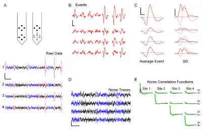
2.1 Event detection and noise analysis on raw tetrode data 27

2.2 Illustration of the SD test on simulated data 40

2.3 Illustration of theχ2 test on simulated data 42

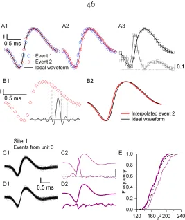
2.4 Sampling jitter 46

2.5 Test of second order noise model 51

2.6 Example of classification on real data 53

3.1 Locust olfactory circuits 61

3.2 PN and KC baseline firing 62

3.3 Tetrode recordings of odor responses in PNs and KCs 64 3.4 Statistics and sparseness of PN and KC odor responses 66 3.5 In vivo sharp-electrode intracellular records from different KCs 70

3.6 Feed-forward inhibition of KCs by LHIs 72

3.7 KC responses to electrical stimulation of PNs 75

3.8 Influence of feed-forward inhibition on KC responses 78 3.9 Extracellular tetrode recordings and spike-sorting 86 3.10 Population responses and sparseness across PNs and KCs 89

4.1 PNs respond to prolonged odor presentations with constant firing 96 4.2 PN responses consist of evolving ensembles of responsive PNs 98

4.3 Visualization of PN population odor responses 102

4.4 Quantification of inter-trajectory distances 106

4.5 Odor information is available from short time slices of single trials 109 4.6 Phase-locked PN spikes show an increased odor response 111

4.7 Idealized odor trajectories 118

A.1 Example of ISI distribution and hazard function 140

A.2 Two statistical tests for PN spike trains 142

A.3 Schematic of hazard model parameters 144

A.4 Statistics from seven simultaneously recorded PNs 146

A.5 Average hazard function statistics 147

(11)

C



1

Introduction

T

  is an information processing device. It takes in information about

the world via an array of sensors, stores and processes the information, and

then sends out signals (information) that control the movement of the body and,

ultimately, behavior. Therefore, to understand how the brain works, it is critical to

understand how information is represented and processed by neural circuits.

1.1

Neural Coding

1.1.1

Distributed population coding

The activity of individual neurons can represent information. Early studies in

elec-trophysiology revealed that in sensory systems, single neurons encode information

about an external stimulus through their level of activity (Adrian, 1926; Hubel and

Wiesel, 1962; Parker and Newsome, 1998). More recently, studies have shown that

the activity of single neurons in motor cortex can control a motor output (Brecht

(12)

neu-rons are responsible for encoding and triggering an escape response (e.g., Roeder,

1948).

Nevertheless, most brain areas are made up of large populations of neurons

and must represent and process more information than any single neuron can

handle. For example, primate primary visual cortex encodes all the basic features

of our entire visual field (color, brightness, orientation, location), and contains over

108 _{neurons. Each neuron’s activity encodes the information contained in only a}

tiny fraction of the entire visual scene, so knowing the activity of just one neuron

is of limited value. For this reason, it makes sense to consider the responses of

populations of neurons as potential units of information representation.

 

Two populations of sensory neurons can represent the same sensory information

in very different ways. In order to describe a particular population coding scheme, it is useful to describe the way each member of the population responds under all

conditions. By presenting a wide range of stimuli and recording the strength of a

single neuron’s response, an experimenter can build a tuning curve for that cell.

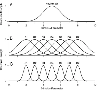
For example, figure 1.1A shows the tuning curve of a hypothetical cell in response

to a range of stimuli that vary along one dimension. In practice this dimension

(represented by parameterp), could correspond to color, sound frequency,

temper-ature, or any other sensory feature to which neurons will respond. In a typical

(13)

Figure 1.1.A, the hypothetical tuning curve for neuron A1. This curve measures the re-sponse intensity (which ranges from 0 to 1) for this neuron, in rere-sponse to a set of stimuli, where parameter pvaries from 0 to 10.B, the tuning curves for a population of neurons (B1–B7) with tuning curves similar toA1, but centered on different values of parameterp.

(14)

Neural populations can be compared on the basis of their average tuning curve

width. Roughly speaking, this corresponds to the range of stimuli that can elicit a

response from one neuron. By comparing the set of tuning curves in figures 1.1B and

1.1C, one can see that the tuning widths of the cells in populationCare narrower

than those of population B. If a stimulus with parameter p = 4 is presented to populationC, only one of the seven cells will be active (C3). In contrast, the same

stimulus presented to population B would elicit some response from over half the

cells. Those responses are both valid representations the stimulus p = 4 for those two particular populations.

In real neuronal populations as well, tuning widths vary substantially across

different cell populations (Ringach et al., 1997) or even over time within the same populations (Spitzer et al., 1988). In many cases, however, it is experimentally

difficult to measure tuning curves. For example, consider a neuron in the visual system that responds to images of 3-dimensional objects; it would be impossible

to present all possible visual stimuli to that cell, or even a reasonable subset. In

such situations, it is often more practical to measure a related statistic, population

sparseness. The sparseness of a population response refers to the total fraction of

cells that are active in response to a stimulus. When this fraction is low, sparseness

is high. Unlike a tuning curve, sparseness can be measured for even a small set of

stimuli. Returning to the simple model in figure 1.1, one can see that the response

of population C is much sparser than that of B (for the reasons explained earlier).

(15)

been around for decades (Barlow, 1969). More recently, experimental results have

shown that sparse codes are found in areas as varied as mammalian visual cortex

(Vinje and Gallant, 2000) and frog olfactory cortex (Duchamp-Viret et al., 1996).

The relative theoretical advantages of population coding with wide or narrow

tuning widths (or sparse or non-sparse codes) have been examined recently (e.g.,

Fitzpatrick et al., 1997), but the results seem to depend critically on the specifics of

the system (e.g., the noise correlation between cells (Pouget et al., 1999)). It is likely

that the manner in which other neurons read out this information will strongly

affect the optimal width of response tuning.

The insect olfactory system provides an ideal system for addressing many issues

relevant to population codes. In the following few chapters, we will study two

con-nected populations of neurons, both in the olfactory pathway, that employ two very

different strategies of population coding. Chapters 3 and 4 will demonstrate that odor representations in the antennal lobe are distributed across a large percentage

of its neurons. In contrast, in chapter 3 we show that the mushroom body, which

receives direct olfactory input from the antennal lobe, has representations that are

significantly more sparse than those in the antennal lobe. By closely examining the

transformation that takes place between these two areas, we are able to uncover

some of the mechanisms that allow a dense code to be read out and converted

into a sparse code. The insect olfactory system is therefore an attractive system for

(16)

1.1.2

Temporal coding

How do nervous systems read out the activity of a single neuron? Up to this point

we have not explicitly defined how to measure the response of a single neuron.

A straightforward way of reading out a neuron’s response is by computing its

mean firing rate within a time window of arbitrary (or reasoned) length (e.g., a

few hundred milliseconds), and tracking how this value changes across successive

time windows. This measure, often described as a rate code, is used in a large

number of experimental systems (Parker and Newsome, 1998). In sensory systems

in particular, the mean firing rate of certain neurons is strongly correlated with one

or more parameters of the stimulus being applied (Adrian, 1926; Hubel and Wiesel,

1962).

In a pure rate code, the only relevant measure is a neuron’s mean rate of spike

generation. The precise timing of any one action potential is not considered

impor-tant.1 Nevertheless, there is an increasingly large body of evidence that suggests

that information can be encoded in the temporal precision of output spikes (Singer,

1999; VanRullen et al., 2005).

The termtemporal codingis used to describe the idea that the precise temporal

patterning of spiking activity may play an important role in neural information

processing. Although the term is often used specifically in the context of synchrony,

for the present manuscript we borrow a more general definition of temporal coding2

from Dayan and Abbott (2001):

1_What_precise_{really means must be defined on a case by case basis.}

2_{A more rigorous and quantitative definition of temporal coding and an exploration of closely}

(17)

Temporal coding refers to (or should refer to) temporal precision in the response that does not arise solely from the dynamics of the stimulus, but nevertheless relates to the properties of the stimulus. (Dayan and Abbott, 2001, p. 38)

Several distinct temporal coding strategies have been proposed, each with

signifi-cant evidence to support its existence in areas of the nervous system.

1. 

Theoretical studies have proposed that synchrony in spike timing across

en-sembles of neurons is used as a signal in the brain (Singer, 1999; Singer

and Gray, 1995). Evidence of synchronous neural activity has been found

across many brain areas in vertebrates and invertebrates alike (Adrian, 1942;

Gelperin and Tank, 1990; Laurent and Naraghi, 1994; Fries et al., 2000).

Never-theless, there is still considerable debate regarding the ability of synchronous

spikes to encode relevant information and about whether that information is

read out by, and relevant to, other neurons.

Direct experimental evidence is difficult to collect, although some studies do address these questions. For example, Schnitzer and Meister (2003) found

that more information can be extracted from synchronous spikes across retinal

ganglion cells than from the spikes of single cells alone. Stopfer et al. (1997)

demonstrated that disrupting synchrony in the insect olfactory system leads

to behavioral deficits. The same manipulation also decreases the response

specificity of the desynchronized cells’ targets (MacLeod et al., 1998;

(18)

2.  

Abeles (1991) proposed the model of asynfire chainthat can generate

repeat-able patterns of spatio-temporal activity in response to an initial stimulus. In

this model, a neural population is wired up so that a small ensemble of

syn-chronously active neurons at one time will, after a short delay, consistently

elicit the synchronous activity of a different ensemble of neurons. Such a net-work can sustain self-perpetuating sequences of activity that are repeatable

for the same initial conditions. Evidence for such self-perpetuating

spatio-temporal patterns of activity has been found in cortex (Abeles et al., 1993;

Ikegaya et al., 2004), though the model remains controversial.

3. - 

Yet another type of temporal code considers the order in which spikes are fired

across a population of cells. Theoretical (Thorpe, 1990, 2001) and experimental

(Johansson and Birznieks, 2004; Petersen et al., 2001) evidence suggest that a

sensory stimulus can be decoded by ranking a population of neurons by the

order in which their first stimulus-evoked spike was fired. A first-spike based

mechanism should decode a stimulus faster than a firing rate based model.

One theme common to all these temporal coding mechanisms is that spike times

are measured relative to the timing of spikes from other neurons in the population.

The absolute timing of a spike with respect to the stimulus is not directly important.

This is a critical feature for a biologically plausible coding scheme because neurons

(19)

the timing of the stimulus itself. This is also an important consideration when

designing an experiment to study temporal coding. Only by recording multiple

neurons simultaneously can one be sure of the relative timing between their spikes.

Because spike timing is relative, temporal coding often requires a population

response.3 _{Temporal information is only relevant with respect to the rest of the}

population. Conversely, by using temporal coding, the total information encoded

by a population of neurons can potentially be more than the information that could

be decoded from each neuron individually.

The work described in the body of this dissertation will explore a system that

uses both population and temporal coding—the insect olfactory system. The next

section of the introduction will provide a brief overview of this system.

1.2

Insect Olfactory System

As a model for studying neural coding, the insect olfactory system offers many benefits. One primary reason for studying insect nervous systems is their relative

simplicity. Although insects can engage in many complex behaviors, including

asso-ciative learning (Heisenberg, 1989; Menzel and Muller, 1996), navigation (Wehner

and Menzel, 1990), and even understanding some high-level concepts (Giurfa et al.,

2001), their nervous systems are much smaller and simpler than mammalian

sys-tems. For example, the first stage of olfactory processing in insects, the antennal

3_{Information can also be encoded in the relative timing among spikes from the same neurons}

(20)

lobe, consists of only two main cell types,4_totalling_∼_{1000 neurons in locust (Leitch}

and Laurent, 1996). In contrast, the analogous structure in mammals, the olfactory

bulb, contains twice as many major neuron types and well over one million total

neurons in rabbit5_{(Shepherd et al., 2004). The large size of many insect neurons, as}

well as their ease of access, allows an experimenter to make in vivo recordings from

many different types of neurons and even record from large numbers of neurons simultaneously.

The olfactory system of insects is an especially attractive system because of

its strong functional and structural homology to the mammalian olfactory system

(for details, see Hildebrand and Shepherd, 1997). In both systems, receptor

neu-ron axons exhibit similarly precise and convergent targeting to specific locations

(glomeruli) in the first olfactory relay (Mombaerts et al., 1996; Vosshall et al., 2000).

This relay, the antennal lobe (AL, insects) or olfactory bulb (OB, mammals), is a

site of significant convergence and divergence in both systems. The AL and OB

contain at least an order of magnitude fewer neurons than both the number of

receptor neurons that provide their input, as well as the number of cells in their

main output regions (mushroom body, piriform cortex) (Hildebrand and Shepherd,

1997). In addition, both insects and mammals (as well as species from other phyla)

exhibit odor-evoked oscillatory activity (Laurent and Naraghi, 1994; Adrian, 1942;

Gelperin, 1999). These similarities provide reason to believe that the coding

princi-4_{In moths and some other species, the projection neurons are further classified into a number of}

subtypes (Homberg et al., 1989).

5_{The rabbit has 150,000 mitral and tufted cells (Allison, 1953) and the number of intrinsic cells}

(21)

ples revealed in insects will not only improve our understanding of neural coding

in general, but may apply directly to our understanding of olfaction in mammals.

1.2.1

Olfactory receptor neurons

 

Olfactory stimuli are transduced by a class of cells known as olfactory receptor

neurons (ORNs). In insects, ORNs are located in chemosensory sensilla, small

cuticular structures, which are found along the antenna, on the maxillary and

labial palps, and elsewhere as well. In locusts, however, olfactory sensilla are found

primarily on the antenna (Chapman, 1998).

Antennal sensilla can be classified into at least four morphological categories,

although not all contain ORNs. In locust, basiconic and trichoid sensilla are known

to be olfactory, and there is evidence that some types of coelconic sensilla also

contain chemosensory neurons (Ochieng et al., 1998; Chapman, 1998).

An olfactory sensillum typically consists of a hair-like or peg-like protrusion of

the cuticle. The cell bodies of the ORNs are located at the base of the sensillum. A

single sensillum will typically contain two or more ORNs. In locust, some basiconic

sensilla are innervated by up to 50 ORNs (Ochieng et al., 1998). The ORNs send

dendrites towards the distal end of the sensillum. The surface of the sensillum

contains a number of pores, 10–25 nm in diameter, that allow odorant molecules

to enter the sensillum and contact receptors on the the outer segment of the ORN

dendrites6(Chapman, 1998).

(22)

The axons of ORNs project down the antenna and innervate the antennal lobe.

In locust these projections are restricted to the ipsilateral antennal lobe, where

they may terminate in a small number of compartments, known as glomeruli (see

section 1.2.2), within the AL (Hansson and Anton, 2000; Hansson et al., 1996).

 

The electrophysiological responses of individual ORNs are typically recorded

ex-tracellularly, by inserting an extracellular electrode into the base of a sensillum

(Kaissling, 1995). During such a recording, the action potentials from multiple

ORNs can be detected, and these are often easily discriminable on the basis of their

shape (de Bruyne et al., 2001).

When ORNs respond to a square pulse of odor, they do so by reaching a steady

tonic firing rate. In many cases, this constant rate is preceded by a transient increase

in firing above the eventual tonic rate (Kaissling, 1971). In addition, some inhibitory

responses have been observed (Kaissling, 1971; de Bruyne et al., 2001), although

less is known about these responses. Unfortunately, very little data currently exist

on ORN responses in the locust (see Hansson et al., 1996, for one example).

The responses of ORNs are highly odor dependent. Most insect ORNs tend

to respond to a small, specific subset of odors (Chapman, 1998; de Bruyne et al.,

2001). In some cases, ORNs respond almost exclusively to one behaviorally relevant

compound, like a pheromone, or the odor of a host plant (Kaissling, 1971).

The specificity of an ORN’s response is conferred, at least in part, by the

(23)

ant receptor (OR) proteins that it expresses. Recent genetic studies in fruit flies

described a family of genes that encode all olfactory receptor proteins (Clyne et al.,

1999; Vosshall et al., 1999). A single ORN expresses only one of these ORs in its

den-dritic membrane7 _{plus a second ubiquitous OR, present in most ORNs (Dobritsa}

et al., 2003; Larsson et al., 2004).

1.2.2

Antennal lobe



The antennal lobe (AL) is the first olfactory relay in the insect brain. Like its

mam-malian counterpart, the olfactory bulb, the AL is composed primarily of spherical

regions of neuropil called glomeruli. The number of glomeruli per AL vary across

different orders of insects. The locust AL contains ∼_{1000 glomeruli (Ernst et al.,} 1977). In comparison, fruit flies have only∼_{43 (Laissue et al., 1999).}

As described in section 1.2.1, glomeruli are the synaptic targets of ORN axons.

The input to each glomerulus is highly specific: in fruit flies, all ORNs expressing

the same OR gene have been shown to target the same one or two glomeruli in the

AL (Vosshall et al., 2000; Mombaerts et al., 1996).

 

Within the glomeruli, ORNs synapse onto the two main cell types of the AL, local

neurons (LNs) and projection neurons (PNs) (Ernst et al., 1977). Local neurons have

neurites that are completely restricted to within the AL. Several different classes

7_{One recent study has found an exception to this rule, a class of ORNs where at least one ORN}

(24)

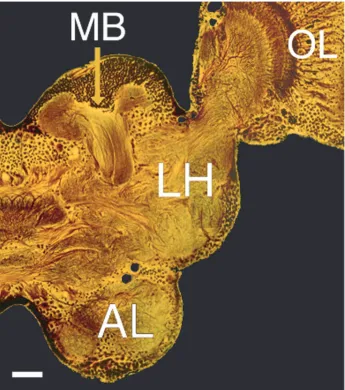
100µm

(25)

of LNs have been observed across species, some innervating the entire AL, some

innervating all the glomerular regions, and others innervating only a small fraction

of all glomeruli (Hansson and Anton, 2000). The locust AL contains ∼_{300 LNs,}

many of which (probably all) arborize widely across the AL (figure 1.2) (MacLeod

and Laurent, 1996).

Local neurons in different insects exhibit a variety of physiological characteris-tics. In some species, like bees and moths, LNs generate sodium action potentials. In

other species, like locusts, LNs show only graded potential responses and calcium

(TTX-resistant) spikes (Leitch and Laurent, 1996; Laurent and Davidowitz, 1994).

In locusts, as in most other insects, LNs are GABAergic (Leitch and Laurent, 1996;

Hansson and Anton, 2000), although there are some reports of excitatory LNs in

other species (Homberg et al., 1989).

 

Projection neurons form the sole output of the AL. In locusts, PNs are cholinergic

and project ipsilaterally, both to the calyx of the mushroom body and to the lateral

protocerebrum (figure 1.2) (Oleskevich, 1999; Ernst et al., 1977). Projection neurons

show similar projection patterns in other insects including fruit flies, cockroach

and moth (Homberg et al., 1989), though not all PNs in these species project to

both locations (Homberg et al., 1989). In fruit flies and bees, for example, some PNs

project only to the lateral protocerebrum (Wong et al., 2002; Flanagan and Mercer,

1989).

(26)

multiglomerular dendritic trees. Locust PN dendrites seem to be very precisely

organized, typically innervating 10–14 co-planar glomeruli, all at roughly the same

radius from the center of the AL (Farivar, 2005). The relationship between the

precise multiglomerular targeting of locust PNs and the multiglomerular targeting

of locust ORNs is not yet known.

PNs in other insect species can be both uniglomerular and multiglomerular

(Hansson and Anton, 2000; Homberg et al., 1989). Populations of both uni- and

multiglomerular PNs have been identified in moth (Homberg et al., 1989), bee

(Fonta et al., 1993), and cockroach (Malun et al., 1993).

The electrophysiological responses of locust LNs and PNs will be described in

section 1.2.4.

 

In some species of insects, a small number of neurons have been identified that

have axon terminals in the AL and dendritic trees in other regions of the nervous

system (Homberg et al., 1989; Hansson and Anton, 2000). These neurons typically

show traces of biogenic amines and are therefore believed to mediate modulatory

feedback (Hansson and Anton, 2000). In honeybees, an identified octopaminergic

centrifugal neuron, VUMmx1, is thought to mediate the encoding of an

uncondi-tioned stimulus (sucrose solution) in an olfactory association task (Hammer, 1993).

At least one octopaminergic centrifugal neuron is known to innervate the locust

(27)

1.2.3

Mushroom body

  

The mushroom body (MB) is a synaptic target of the PNs. The MB is primarily

composed of intrinsic cells called Kenyon cells (KCs). In locust, KC cell bodies

are quite small (3–8µm, Laurent and Naraghi, 1994), and∼_{50,000 KCs are tightly}

packed above the MB calyx, the input region of the MB (see figure 1.2). Each KC

sends a primary neurite into the cup-shaped calyx. There the neurite bifurcates and

forms a dendritic tree spanning a small fraction of the entire calyx (Farivar, 2005).

Projection neuron axons terminate throughout the main calyx (Farivar, 2005), which

suggests that the majority of KCs receive some PN input. In other insect species,

KCs are known to receive calycal inputs from other modalities as well (Gronenberg,

1999; Strausfeld et al., 1998).

Kenyon cell axons leave the calyx and proceed to the pedunculus, a dense

bun-dle of KC axons, which show conspicuous reciprocal synaptic connections between

neighboring axons (Leitch and Laurent, 1996). At the end of the pedunculus, KC

axons bifurcate and terminate in both theα- andβ-lobes, where they form synapses

onto MB extrinsic neurons. These extrinsic neurons exhibit a wide variety of

branch-ing patterns. Many of these neurons have been shown to innervate the MB calyx

or pedunculus as well as the lobes (Farivar, 2005; MacLeod et al., 1998; Li and

(28)

  

There are very few published examples of electrophysiological recordings of KCs

(Laurent and Naraghi, 1994; Erber et al., 1987). Nevertheless, the MB has been

strongly implicated in olfactory learning and memory (Heisenberg, 2003). In flies,

MB ablation (both genetic and chemical) leads to deficits in olfactory memory

(Heisenberg et al., 1985; de Belle and Heisenberg, 1994). Similarly, many

muta-tions of genes expressed in KCs (e.g.,rutabaga, amnesiac) impair olfactory learning

behavior (Heisenberg, 2003).

1.2.4

Synchrony and olfactory coding

Recent electrophysiological studies in the locust AL and MB have revealed several

basic characteristics of their odor responses. The most prominent component to

the response is an odor-evoked rise in synchronized oscillatory activity at∼_{20 Hz.}

Odor-evoked oscillations have been observed in many other species (Adrian, 1942;

Gelperin, 1999) and, as in these other systems, they can be observed in the locust

by recording local field potentials (LFPs) (Laurent and Naraghi, 1994). Moreover,

intracellular recordings from PNs, LNs and KCs all reveal odor-evoked

subthresh-old oscillatory activity that is phase-locked with the LFP oscillations (Laurent and

Davidowitz, 1994; MacLeod and Laurent, 1996; Laurent and Naraghi, 1994).

In PNs, there is a second component to the odor response, consisting of

alternat-ing periods of excitation (spikalternat-ing) and inhibition. These epochs change at a slower

(29)

slow responses are odor- and PN-specific. Individual spikes during these PN

re-sponses all tend to lock to the same phase of the LFP oscillations (Wehr and Laurent,

1996). Thus odor-evoked spikes across the population of PNs tend to synchronize

with one another.

Kenyon cells also show odor- and KC-specific firing patterns. Like PN spikes,

odor-evoked KC spikes tend to lock to a single phase of the LFP (Laurent and

Naraghi, 1994).

Fast GABAergic inhibition in the AL was shown to underlie the odor-evoked

oscillations (MacLeod and Laurent, 1996). In the same study, MacLeod and

Lau-rent (1996) demonstrated that by applying picrotoxin (PCT), a GABA antagonist,

to the AL, odor-evoked oscillatory synchrony could be abolished. Moreover, the

slow component of the PN responses, including periods of inhibition, remained

unchanged. This discovery paved the way for two different studies that examined the importance of synchrony.

MacLeod et al. (1998) studied the effects of AL synchrony on odor responses inβ -lobe neurons. These neurons receive olfactory input from KCs, which in turn receive

direct PN connections. The odor responses ofβ-lobe neurons were evaluated before

and after PCT injection in the AL. After injection—and therefore after the abolition

of oscillatory synchrony—responses changed substantially.β-lobe neurons began

responding to new odors (their tuning curves became wider), and their responses

to different odors became more similar—and therefore less informative.

(30)

behav-ioral consequences of synchrony disruption. Bees were trained to discriminate

between pairs of odors, using a behavioral paradigm. Bees treated with PCT

in-jections showed a significant deficit in discriminating similar odors. Their ability

to discriminate dissimilar odors remained unimpaired. Taken together these

re-sults demonstrate the critical role of oscillatory synchrony in the functioning of the

olfactory pathway.

1.3

Outline and Specific Aims

The focus of this dissertation is to characterize and quantify the features of the

neural population code in the insect antennal lobe. Specific emphasis will be given

to temporal aspects of the code. This work relies heavily on and extends previous

work on olfactory coding in the locust (e.g., Wehr and Laurent, 1996; MacLeod

and Laurent, 1996; Laurent, 1999; Laurent and Naraghi, 1994). These studies

ele-gantly worked out some of the fundamental principles of the AL’s odor responses,

including describing two different time scales of odor-evoked temporal dynamics. Simultaneous recordings of many PNs were necessary to precisely characterize

the temporal components of the PN population response (see section 1.1.2), as well

as to establish a large database of PN responses. Thus, the majority of the data

presented in the following chapters were collected with multi-unit, multi-channel

extracellular recordings. Multi-unit extracellular recordings present a unique

chal-lenge because no single fool-proof method exists for unambiguously extracting the

(31)

spike-sorting. Adapting a rigorous spike-sorting algorithm was a necessary

pre-requisite to addressing neural coding questions. Chapter 2 will present several

ad-vances in the algorithms for analyzing the raw data from multi-unit, multi-channel

extracellular recordings. One major advance is the development of quantitative

statistical tests to assess the output quality of the spike-sorting. These tests are

modular and can be adapted to other spike-sorting algorithms. A second advance

presented in chapter 2 is the use of the statistics of recording-noise to optimize the

clustering stage of the spike-sorting algorithm and allow it to be automated. The

noise statistics are then used again in the post-sorting quality tests. The work in

chapter 2 was published as Pouzat et al. (2002).

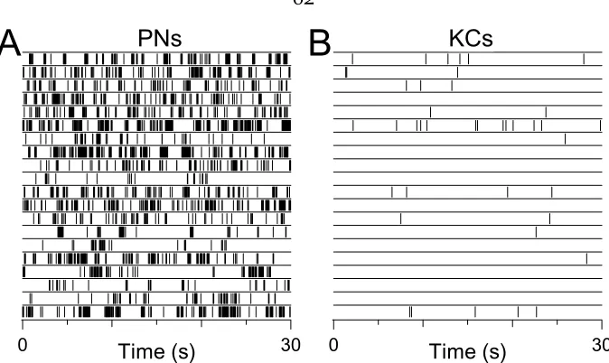
Chapter 3 quantifies some of the key differences in the population codes of the first two olfactory relays in the insect brain, the AL and the MB. The results show

that the odor code in the KCs (of the MB) is significantly more sparse than that of

PNs (of the AL), even though KCs receive direct excitatory input from PNs. The

second part of chapter 3 addresses the mechanism underlying this striking

trans-formation. The results point to several different underlying components, including oscillatory dynamics, feed-forward inhibition and intrinsic properties of the KCs

that all work together to bring about this change. Among the conclusions of this

work is that a single oscillation cycle (∼_{50 ms) is the relevant time scale for this}

transformation. The work presented in chapter 3 was published as Perez-Orive

et al. (2002).

(32)

population response of the PNs. The work in this chapter addresses some of the

questions brought up by chapter 3, including the degree of PN synchrony over

the course of an odor response, the fraction of PNs that respond during a single

oscillation cycle, and the degree to which the PN population response changes

from one oscillation cycle to the next. The results further explore the dynamics

of the PN population response and describe three separate phases to an odor

response. There are distinct responses to the onset and the offset of an odor pulse, both characterized by periods of strong odor-specific dynamics. Additionally, in

response to odor durations longer than∼_{2 s, the PN population reaches a state of}

constant activity. While still to some extent odor-specific, this period is shown to

be substantially less informative about odor identity than the transient response

(33)

C



2

Using Noise Signature to Optimize

Spike-Sorting and to Assess Neuronal

Classification Quality

U

   will, as a prerequisite, likely require the

simul-taneous sampling of large populations of neurons. While many powerful

imaging techniques have been developed (e.g., membrane voltage (Wu et al., 1994);

intrinsic signal (Frostig et al., 1990); fMRI (Ogawa et al., 1992)), extracellular

record-ing remains the only method that provides both srecord-ingle neuron and srecord-ingle action

potential resolution from large and distributed samples. Multi-neuron extracellular

recordings, however, are useful only if the spikes generated by different neurons can be sorted and classified correctly. Although a given neuron may generate spikes

with unique extracellular signal features, making the identification issue trivial, in

most cases, the electrophysiologist must, from noisy and ambiguous primary data,

answer the following questions:

1. What is the waveform generated by each neuron, orunit, on each recording

(34)

2. How many units were sampled by the recording?

3. On what objective basis should an individual event, or spike, be classified as

originating from one of the units sampled?

4. How should superpositions, due to the nearly simultaneous occurrence of

two (or more) spikes, be resolved?

5. How likely are misclassifications, that is, how often is an event generated by

neuron A classified as originating from neuron B, and vice versa?

6. How can we test and quantify objectively the reliability of our classification

procedure?

The first three questions have been the focus of much investigation and several

methods have been proposed (reviewed by Lewicki, 1998), such as principal

com-ponent analysis (Glaser and Marks, 1968), Bayesian classification (Lewicki, 1994),

clustering based on the expectation-maximization algorithm (Sahani, 1999),

tem-plate matching (Millecchia and McIntyre, 1978), wavelet transform based methods

(Letelier and Weber, 2000; Hulata et al., 2000) and clustering methods that use spike

time information to determine cluster boundaries (e.g., Fee et al., 1996a). Question

4 has been directly addressed in two studies (Atiya, 1992; Lewicki, 1994). The

re-liability of some of these spike-sorting procedures has also recently been tested

empirically, using simultaneous extra- and intracellular recordings (Wehr et al.,

1999; Sahani, 1999; Harris et al., 2000). These later studies fail to address the main

(35)

alone, the reliability of the sorting procedure? The potential causes of unreliable

spike-sorting are numerous; several are described in detail by Lewicki (1998).

Ac-cording to Lewicki (1998, p. 74), “Many algorithms work very well in the best case,

when most assumptions are valid, but can fail badly in other cases. Unfortunately,

it can be difficult to tell which circumstance one is in.” The simple tests we present here are an attempt to address this dilemma.

In the body of the paper, we will provide a detailed description of our methods,

as well as an illustration of their use on in vivo recordings from locust antennal lobe

neurons. We begin by presenting a brief description of the experimental procedure

including data collection. Next, we describe the method for generating a model of

the experimental noise and for testing the accuracy of the model. We then proceed

to show how that model can be used first to cluster spikes, and then to test the

quality of the classification. Finally, we run the entire procedure on an example of

real data.

2.1

Methods

2.1.1

Data collection and representation

  

All experiments were carried out on adult locusts (Schistocerca americana) of both

sexes, taken from a crowded colony and prepared as described by Laurent and

Naraghi (1994).

(36)

Commu-nication Technology of the University of Michigan (Drake et al., 1988). A diagram

of the probe tips with 16 recording sites is shown in figure 2.1A. The probe was

connected to a custom-made impedance-matching preamplifier. The preamplifier

was connected to two 4-channel differential AC amplifiers (AM model 1700 AM Systems Inc.; Carlsborg, WA). The signals were bandpass filtered between 300 and

6000 Hz and amplified 10,000 times. Data were acquired at 15 kilosamples per

second using a 12 bit A/D card (Win30 D, United Electronics Inc., MA).

Data with a good signal to noise (S/N) ratio were collected relatively close to the surface (50–100µm) of the antennal lobe (AL). Spikes recorded in the AL were

attributed to the activity of projection neurons (PNs), as the AL contains only two

neuron populations: the PNs, which are the output neurons and fire Na+ action

potentials and the local neurons (LNs), which are axonless and fire no Na+ action

potential (Laurent and Davidowitz, 1994). We were unable to record clear spikes

with the silicon probe from the antennal nerve or its projections into the AL. Afferent axons are very small and numerous (90,000), precluding clear discrimination of

single neuron signal from noise.

 

Data were analyzed offline on a PC computer (Pentium III 550 MHz, 256 MB RAM) using Igor (WaveMetrics, Lake Oswego, OR) or Scilab (a free Matlab-like software

package available at: www-rocq.inria.fr/scilab). All the routines were custom

developed (or are freely available on the world wide web, see below) and are

(37)

(38)

 

For the detection stage only, the traces were first digitally smoothed (3-point box

filter). Events (i.e., putative spikes) were then detected as local maxima with a

peak value exceeding a preset threshold. In cases where the spike peak occurred at

slightly different times on different recording sites, only one time value was used: the time from the site with the largest peak amplitude. The detection threshold was

set as a multiple of the standard deviation (SD) of the whole trace. We typically

used thresholds between 2.25 and 3.5 SDs.

 

Detected events can be represented in many different ways (Lewicki, 1998). Yet, the choice of a representation can strongly influence both the speed and the reliability

of the classification procedure. In general, one measures a set ofDparameters for

each event; each event thus becomes a point in aD-dimensional space. This space is

calledevent space. Our goal was to optimally predict the effect of recording noise on the distribution of points that represent events in event space. Unfortunately,

sev-eral common parameter choices, such as peak and valley amplitudes or half width

are computed by differentiating the raw data. This makes signal-noise separation difficult.

We therefore chose to represent each event as follows. A sweep ofdconsecutive

sample points around the peak of the event was examined from each recording

(39)

successive amplitudes of an event on site A,A1A2...A45, on site B,B1B2...B45, on site

C,C1C2...C45 and on site D,D1D2...D45, the vector representing the event was:

e=(A1...A45B1...B45C1...C45D1...D45)T,

where the superscriptTmeans transpose. For our purposes, therefore, the

dimen-sionality of the event space, D, is 180 (4×_{45). It will become clear that with this}

choice of event space, the effect of noise on the distribution of events can be easily predicted. Note that our initial peak detection for event selection introduces some

sampling-induced jitter. We will ignore this for now and show later how it can be

canceled.

    

Following Lewicki (1994) and Sahani (1999), we use an explicit model for data

generation. The general assumptions in our model are:

1. The spike waveforms generated by a given neuron are constant.

2. The signal (i.e., the events) and the noise are statistically independent.

3. The signal and noise sum linearly.

4. The noise is well described by its covariance matrix.

Assumption 1 is a working approximation, appropriate for some documented

cases (Fee et al., 1996b, figure 2; Harris et al., 2000, figure 4). It also applies to our

(40)

are implicit in most already available spike-sorting methods and mean that the

amplitude distribution of the recorded events can be viewed as the convolution of

a pure signal with the noise distribution. We can restate our hypothesis as follows:

in a noise free recording, all events generated by one unit would give rise to the

samepoint in event space. In a noisy recording, however, events generated by one

unit would give rise to a cloud of points centered on a position representing the

ideal waveform of the unit. The distribution of the points should be a multivariate

Gaussian whose covariance matrix would be the noise covariance matrixregardless

of the position of the unit in event space.

2.1.2

Noise model

  

To measure the statistical properties of the noise, we began by removing from the

raw traces all the detected events (i.e., all the d-point sweeps) and concatenating

all the inter-event traces. We call the resulting waveforms “noise traces” (see

fig-ure 2.1D). The auto-correlation function was then calculated for each recording site

(diagonal, figure 2.1E), as were the cross-correlation functions between all pairs

of sites (figure 2.1E). These correlations were only computed within continuous

stretches of noise (i.e., the discontinuities in the noise traces due to eliminated

spikes were skipped). In addition to recording noise, these cross-correlations will

also account for any cross-talk between recording channels (Zhu et al., 2002).

(41)

covariance matrix which was built by blocks from these functions as follows (we

refer here to the four recording sites as site A, B, C and D):



where each block is a symmetric Toeplitz matrix build from the corresponding

correlation function (e.g., AA is a 45 × _{45 matrix whose first row is the noise}

autocorrelation function on site A, AB is a 45×_{45 matrix whose first row is the}

noise cross-correlation function between sites A and B, etc). BAis symmetrical to

AB.1

 

In order to simplify calculations and reduce the computational complexity of our

algorithm, we chose to make a linear transformation on our event space (and

there-fore on all the detected events). The transformation matrix,U, is chosen specifically

so that after transformation, the variance due to noise will be uncorrelated across

dimensions (i.e., the noise covariance matrix will be the identity matrix,I).

Mathe-1_{For readers unfamiliar with Toeplitz matrices, we illustrate the concept using the simple case}

(42)

matically,Uhas the property that

Γ−₁

=UTU, (2.1)

whereΓis the noise covariance matrix in the original event space. A transformation matrix,U, with this property will always exist as long as the covariance matrix (Γ) is symmetric and positive definite (which it is by definition). The matrix U is

obtained from Γ−₁

with a Cholesky decomposition (Brandt, 1999, pp 479–484). A

critical feature of the noise-whitened event space is that if our assumption (4) is

correct (that the noise is well described by its second-order statistics), then the

variance due to noise will be the same in every dimension with no correlations

across dimensions (i.e., the cloud due to noise should be a hypersphere).

   

To test assumption (4), we generated a large sample of d-point long events from

the noise traces. These noise events were taken from a portion of the noise traces

different from the portion used used to calculate the noise covariance matrix. Since these events should contain all noise and no signal (i.e., no spikes), these points

will form a cloud around the origin in the noise-whitened event space and the

distribution of these points around the origin will be fully described by the true

statistics of the recording noise. We can now test if the second-order noise statistics

(43)

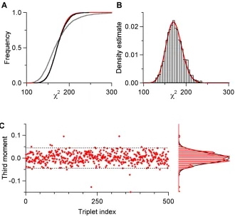
distance squared in noise-whitened space), between each noise event and the origin.

In a white, Gaussian distribution, the distribution of Mahalanobis values will be a

χ2_{distribution with}_D_{degrees of freedom. For our data, as we will describe in the}

results section, this is indeed the case.

Testing the second-order statistics is not a guarantee that the noise distribution

does not have significant higher-order moments. To check for this possibility, we

measured the third momentum distribution from another pool of whitened noise

events. We randomly selected 500 (or more) triplets of coordinates among the 1803

possible ones (for an event space of 180 dimensions). If we writeni =(ni,1, ...,ni,180)T

the ith sweep of the noise sample and if, for example, (28, 76, 129) is one of the

triplets, the third moment for that triplet is obtained as follows (assuming a noise

sample of size 2000):

1 2000

2000

X

i=1

ni,28·ni,76·ni,129.

We will show in the results that for our data, this statistic was not significantly

different from zero.

2.1.3

Noise model-based clustering

   

If our first assumption about data generation is correct (that spike waveforms

are constant), the distribution of events in event space, after the linear coordinate

(44)

(hyper-spheres), each centered on its underlying unit.2 _{Our goal is now to determine the}

number of such clouds and the position of their centers in event space.

To this end, we introduce a specific data generation model (M) that extends

the general data generation model by specifying the number of units, K, their

waveforms and their discharge frequencies. In event space, the waveforms of theK

units translate into a set ofKvectorsuj(joining the origin to the point representing

unit j,j∈ {₁, ...,_K}_{). Our goal is to find the model that gives the best explanation of}

the data sampleS={_e₁, ...,_e_N}_{. A common and e}ffi_{cient way to do this is to find the} model which maximizes a posteriori the probability to observe the sample actually

observed, i.e., to maximize the likelihood function (Brandt, 1999; Bishop, 1995).

The likelihood function is computed under our assumptions and in the

noise-whitened coordinate system as follows. We first compute the probability (density)

for unituj to have generated eventei, p(ei|uj). For that we introduce the residual

vector∆i j:

∆i j =ei−uj,

then

p(ei|uj)=

1 (2π)D2

·_exp₍−1 2·∆

T

i j∆i j). (2.2)

The probabilityPifor the model to have generated eventei can now be written

as a weighted sum of terms like equation 2.2, one for each of the K units of the

(45)

model:

where πj is the probability for unit j to occur, i.e., the ratio of the number of

events from unit jto the total number of events in the sample,N. The a posteriori

probability to observe the sample is then, assuming independence of theNsample

elements, the product of the probabilities to observe each one of them separately:

P₍_S_;_M₎=

N Y

i=1 Pi.

The likelihood function is simply the logarithm ofP_:

L₍_S_;_M₎=

N X

i=1

ln(Pi).

Several iterative algorithms exist to maximize L _{(Redner and Walker, 1984;}

McLachlan and Krishnan, 1997). We used the expectation-maximization algorithm

(EM algorithm, formalized by Dempster et al., 1977, and introduced in the

elec-trophysiological literature by Ling and Tolhurst, 1983). The EM algorithm is very

simple in the present context, fairly intuitive (Bishop, 1995) and its convergence

to local maxima has been proven for the present model (without outliers in the

sample: Boyles, 1983; Wu, 1983). Moreover, for our typical data samples, outliers

do not appreciably affect the speed or accuracy of the algorithm.

The standard EM algorithm finds the best model for a given number of units.

(46)

sample. Several criteria have been proposed in the statistical literature to perform

this task (for an overview, see Fraley and Raftery, 1998 (especially section 2.4), and

Biernacki and Govaert, 1998). Among the methods we tried, however, we found

that the Bayesian Information Criterion (BIC), proposed by Schwarz (1978), worked

well for our data (where most clusters are well separated in event space). The BIC

penalizes an increase in the number of components by subtracting fromL _{a term}

proportional to ν· _ln₍_N_{), where} _N _{is the number of sample events and} ν _{is the}

number of model parameters. We then simply keep the model with the value ofK

which maximizes the BIC (Fraley and Raftery, 1998).

 

Once a model is established, we attribute each event, ei to one of the K units,

by finding the j that minimizes|∆_{i j}|2_{. The rationale is the following: if unit}_u_j _has indeed generated eventeithen the components of the residual vector∆i jare random

numbers drawn from a multivariate Gaussian distribution and the probability to

observe |∆_{i j}|2 _{= ∆}T

i j· ∆i j is given by a χ2 distribution with D degrees of freedom

(assuming noise whitening has been performed). By choosing the unit producing

the smallest|∆_{i j}|2 _{we are simply choosing the unit with the highest probability to}

have generated the event.3

For some events, even the smallest |∆_{i j}|2 _{was very unlikely given the}_χ2

distri-bution (e.g., in the 99th percentile). In these cases, we looked for the superposition

3_{Strictly speaking, we should choose the unit giving the largest product}_πj_·_p₍_e

(47)

of any two units, e.g.,uj and ul, which gave the smallest|∆i,j+l|2value. To this end

we tested all possible pairs of units and all relative timings of their peaks. This was

easily computed for we knew the entire waveform of each unit. This approach was

formalized by Atiya (1992) and an alternative method to resolve superpositions

has been proposed by Lewicki (1994). If, after this step, we still did not find a small

enough|∆_i_,_j₊_l|2_{, we classified the event as an outlier.}

2.1.4

Model verification tests

No matter how much effort is devoted to optimizing model-generation and event-classification procedures, in the end it is always possible for the results of a

spike-sorting routine to be sub-optimal. In many recordings there may be pairs of neurons

whose spike waveforms are close enough (with respect to the size of the noise)

that their events could never be accurately distinguished. In such a case, some

algorithms may lump the pair into one cluster and others might split such a pair

in two. In either case, an experimenter would like to detect such a situation, and

if the pair of units is really inseparable, discard the spikes from those cells or treat

them as multi-unit data. Furthermore, due to the complexity of the task, even the

best algorithms will occasionally generate incorrect models when given reasonable

data. Again, this is a situation one would like to detect.

For this reason, we developed three tests for assessing the quality of

spike-sorting results on a cluster-by-cluster basis. Since we have a quantitative model of

(48)

of our classified data. Here we illustrate the tests’ principles by applying them to

simulated data. In the results section we will present the same test applied to real

data.

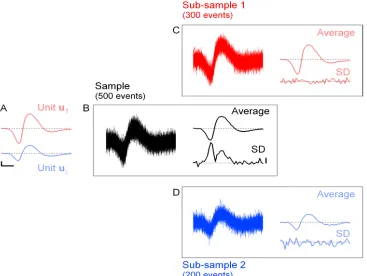
Consider the simple situation in which we record from a single site and where

only two units, u1 and u2, are active. Assume also that both units fire at low

rates, so that nearly simultaneous spikes from unitu1andu2are rare. The original

waveforms of the two units (used to generate the data) are shown in figure 2.2A.

During our “recording session”, we sample 500 events, superimposed in figure 2.2B

(left). Each event corresponds to one of the units, to which random noise drawn

from a normal distribution has been added to each of the 45 sampling points.

This artificial data generation procedure is such that our model assumptions apply

exactly to the sample (in this case, the noise is already white). In this sample, 300

events have been generated from unitu1 and 200 from unitu2.

For the first two tests, we will consider two potential models of data generation.

In the first case, all events of the sample are (incorrectly) classified as coming from

a single unit; in the second case, the data generation model contains the two units

u1andu2, and all events are correctly classified.

  

The mean event and the SD computed from all 500 events of the sample are shown

on the right of figure 2.2B. Note how the SD varies, reaching maxima at times when

the two waveforms (u1 and u2) differ the most. Based on our initial assumptions,

(49)

unit. If this were the case, all the spike-to-spike variance would be due to noise,

which should be constant throughout the time course of the spike.

If we now split the sample into two correctly classified sub-samples, one

con-sisting of the 300 events generated by unit u1 and the other from the 200 events

generated by unit u2, the SD computed on the corresponding subsamples is now

flat, centered on the background noise level (figures 2.2C and D). This matches

precisely with what our model predicts for correctly classified clusters: all the

spike-to-spike variability is due entirely to noise.

In this way, we can use this as a qualitative test of both the accuracy of the

model and a proper classification of the events.4 _{After the events have been}

clas-sified, the SD of every cluster can be tested. Any cluster whose SD values deviate

significantly from the SD of the noise can be eliminated from further analysis (or

at least scrutinized more closely). In our experience, this test is quite sensitive and

can routinely detect clusters that contains multiple units, even if those units are not

well-separable (see projection test).

As a final note, this test will also reliably indicate if a significant number of

spikes from a small unit were not detected. This situation can arise when the peak

voltage of a unit’s waveform is just at the spike detection threshold. In such a

case, a significant percentage of that unit’s events will not be detected due to noise

fluctuations. The spikes from this unit that are detected will have positive noise

values near the peak, and therefore less noise variability along this portion of the

waveform. This situation is therefore characterized by a dip in the SD near the peak

(50)

Figure 2.2.Illustration of the SD test on simulated data.A, waveforms of the two units used to generate the data (see text). The scale bars are arbitrary. The vertical bar has the value 1, equal to the noise’s SD. To compare with real data, the length of the horizontal bar would be 0.5 ms; dashed line at zero.B left, 500 events generated from the two units (300 fromu1

and 200 fromu2) by adding normal white noise to the units waveforms.B top right, average

event computed from the 500 events of the sample.B bottom right, SD computed from the sample. Dotted line, 1 (expectation from the noise properties). Vertical scale bar, 0.1. Notice the non-zero SD at the peak and valley of the average event.C and D, as inB, except that

CandDhave been built from the sub-samples generated by unitu1 andu2, respectively.

(51)

of the waveform, and we routinely observe this effect empirically. Hence, a cluster that exhibits a constant SD, equal to that of the noise, is consistent with a good

model together with correct spike detection and classification.

χ2

In this test we test the prediction that each cluster of events forms aD-dimensional

Gaussian distribution. For every unit,uj, we can compute the distance from it to

all events,ei, that were attributed to it. If the prediction is accurate, the distribution

of the squares of these distances should follow aχ2 _{distribution with}_D_{degrees of}

freedom.

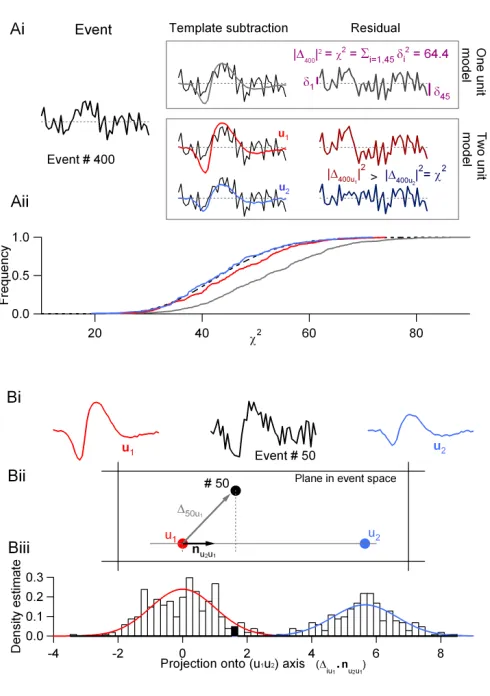
The test is illustrated in figure 2.3A. In the first case (one-unit model), we

take the sample mean as an estimate of the ideal underlying unit. We illustrate

the computation of the residual of event # 400 with such a model (figure 2.3Ai).

Because we have 500 events in the sample, we obtain 500χ2_{values. In figure 2.3Aii}

we plotted the cumulative distribution of these 500 χ2 _{values (continuous gray}

curve). This empirical distribution can be compared with the expected one (dashed

black curve). In this case, the expected distribution is aχ2 _{distribution with} _D₋₁

degrees of freedom (i.e., 44), for we have used the average computed from the same

sample.

In the second case (two-unit model), we take the averages computed from the

two subsamples as estimates of the underlying units (figures 2.2C and D). The

classification of event # 400 is illustrated in the middle part of figure 2.3Ai. In

(52)

Figure 2.3.A, illustration of theχ2 test using the same computer generated sample as in figure 2.2.Ai, one-unit model (top): the average event is first subtracted from event # 400, to yield the residual. The integral of the square of the residual is theχ2value of event # 400. Two-unit model (bottom): two units could now have generated event # 400; the waveforms of these units are given by templatesu1andu2(see text). The integrals of the square of the

two residuals (|∆₄₀₀_u

1|

2 _and_|_∆ 400u2|

2_{) are compared; the smallest indicates which one of}

the two units most likely generated the event, with its associatedχ2value.Aii, cumulative distributions of theχ2 values under the one- and two-unit model assumptions and their expectation (dashed line). Grey line: one-unit model (n= 500); red line: unitu1, two-unit

model (n=300); blue line: unitu2, two-unit model (n=200).B, projection test.Bi, template

u1 (red), u2 (blue) and event # 50 from the 500 computer generated samples. Bii, same

objects in the plane that contains all three points. The straight line joining the two units has been drawn as well as the unit vector originating inu1,nu2u1. The vector joiningu1to

event # 50,∆50u1(representation of the residual in event space) has been drawn as well.Biii,

projection histogram of the 500 events of the sample. The bin containing the projection of event # 50 has been filled. The red curve is probability density function (PDF) expected from the projections of the 300 events generated by unit u1 (60% of the sample) while

(53)

expected to cause such a large deviation from the underlying unit) so the event

is classified as originating from unit u2. We thus obtain from the 500 events, two

empirical χ2 distributions (figure 2.3Aii), one corresponding to subsample 1 (red

curve) and one corresponding to subsample 2 (blue curve). It is clear that these two

empirical distributions are much closer to the expected one. A good classification

(together with a good model) should thus yieldK distributions, for a model with

Kunits, centered on a single predictable χ2_{distribution. Like the SD test, this test}

is especially sensitive to the grouping of two similar-looking units into a single

cluster and will produce a significant rightward shift in such situations.

  

According to our model assumptions, the events generated by a given unit should

form a cloud of points centered on the unit in event space. The precise distribution

of these points should be, after noise-whitening, a multivariate Gaussian with a

covariance matrix equal to the identity matrix. Moreover, the projections of two

subsamples onto