Automatic Feature Selection for Agenda-Based Dependency Parsing
Miguel Ballesteros
Natural Language Processing Group Universitat Pompeu Fabra
Barcelona, Spain
Bernd Bohnet School of Computer Science
University of Birmingham Birmingham, United Kingdom
Abstract
In this paper we present an in-depth study on automatic feature selection for beam-search depen-dency parsers. The search strategy is inherited from the one implemented in MaltOptimizer, but searches in a much larger set of feature templates that could lead to a higher number of combina-tions. Our models provide results that are on par with models trained with a larger set of feature templates, and this implies that our models provide faster training and parsing times. Moreover, the results establish the state of the art for some of the languages.
1 Introduction
Finding an optimal and accurate set of feature templates is crucial when training statistical parsers; in fact it is essential when building any machine learning system (Smith, 2011). In dependency parsing, the features are based on the linguistic information that is annotated within the words and the information that is being calculated during the parsing process. Researchers normally tend to include a large set of feature templates in their machine learning models, following the idea that more is always better; however some recent research on feature selection for transition-based parsing (Ballesteros, 2013; Ballesteros and Nivre, 2014) and graph-based parsing (He et al., 2013) have shown that more features are not always better, at least in the case of dependency parsing; models containing more features are always slower in parsing and training time and they do not always provide better results.
This indicates that a smart feature template selection could be the key in the trade-off for finding an accurate and fast feature model for a given parsing model. On the one hand, we want a parser that should provide the best results possible, while on the other hand, we want a parser that should provide the results in the fastest way possible. For practical applications, a fast model is crucial.
In this paper, we report the results of feature selection experiments that we carried out with the in-tention of obtaining accurate and faster feature models, for the transition-based Mate parser with and without graph-based completion models. The Mate parser is a beam search parser that uses a hash kernel for training, joint part-of-speech tagging, morphological tagging and dependency parsing. As a result of this research, we provide a framework that allows to find an optimal feature template set for the Mate parser (Bohnet et al., 2013). Moreover, our models provide some of the highest results ever reported for a set of treebanks.
The paper is organized as follows. Section 2 describes related work including the used agenda-based dependency parser. This section depicts the feature templates that can be used by a transition-based or a graph-based parser. Section 3 describes the feature selection algorithm that we implemented for our experiments. Section 4 shows the experimental set-up. Section 5 reports the main results of our experi-ments. Section 6 provides the parsing times and memory requireexperi-ments. Finally, Section 7 concludes.
This work is licenced under a Creative Commons Attribution 4.0 International License. Page numbers and proceedings footer are added by the organizers. License details:http://creativecommons.org/licenses/by/4.0/
Transition Condition
LEFT-ARCd ([σ|i, j], B,Γ)⇒([σ|j], B,Γ[(j, i)∈A, δ(j, i)=d]) i6= 0
RIGHT-ARCd ([σ|i, j], B,Γ)⇒([σ|i], B,Γ[(i, j)∈A, δ(i, j)=d])
SHIFTp,m,l (σ,[i|β],Γ)⇒([σ|i], β,Γ[π(i)=p, µ(i)=m, λ(i)=l])
SWAP ([σ|i, j], β,Γ)⇒([σ|j],[i|β],Γ) 0< i < j
Figure 1: Transition set for joint morphological and syntactic analysis. The stackΣis represented as a list with its head to the right (and tailσ) and the bufferBas a list with its head to the left (and tailβ).
2 Related Work 2.1 Mate Parser
For our experiments, we used the transition-based parser of Bohnet et al. (2013). This parser performs joint part-of-speech tagging, morphological tagging, and non-projective labeled dependency parsing. The parser employs a number of techniques that lead to very competitive accuracy such as beam-search with early update (Collins and Roark, 2004), a hash kernel that can quickly cope with a large feature set, a graph-based completion model that adds scores for tree parts which a transition-based parser would not be able to consider, cf. (Zhang and Clark, 2008; Bohnet and Kuhn, 2012). The graph-based model takes into account second and third order factors and obtains a score as soon as the tree parts are completed. The parser employs a rich feature set for a transition-based model (Zhang and Nivre, 2011; Bohnet et al., 2013) as well as for a graph-based model. In total, there are 326 different feature templates for the two models. The drawback of such a large feature set is a huge impact on the speed. Important research questions include (1) whether the number of features could be reduced to speed up the parser and (2) whether languages dependent feature sets would be beneficiary.
2.2 Features in transition-based dependency parsing
Every transition-based parser uses two data structures: (1) a buffer that contains at the beginning of the parsing process all words of the sentence that have to be parsed, and (2) a stack.
The Mate parser that we used in our experiment follows Nivre’s arc-standard parsing algorithm plus the SWAP transition to build non-projective dependency trees. Figure 1 depicts the transition system
formally; the SHIFT transition removes the first node from the buffer and puts it on the stack. The LEFT-ARCdtransition introduces a labeled dependency edge between the top element on the stack and
the second element of the stack with the labeld. The second top element is removed from the stack. The RIGHT-ARCdtransition introduces a labeled dependency edge between the second element on the
stack and the top element with the labeldwhile the top element is removed from the stack. TheSWAP
transition swaps the position of the topmost nodes of the stack and the buffer.
A classifier selects transitions based on the feature templates that are composed of stack elements, buffer elements, the already created parse, and the transition sequence. For instance, if the parser contains the feature template LEMMA(S1), it means that it may use the lemma of the word that is in the first position of the stack in any parsing state in order to select the best parsing action.
2.3 Features in graph-based dependency parsing
vertexes involved in the factors. A feature template of a second order factor is composed of properties drawn from up to all three vertex, e.g., the part-of-speech of the head, the dependent and a child denoted as POS(H)+POS(D)+POS(C). In our experiments, we use in addition to the transition-based model, a
completion model that uses graph-based feature templates with up to third order factors to re-score the beam.
2.4 Feature Selection
There has been some recent research on trying to manually find better feature models for dependency parsers, such as Nivre et al. (2006), Hall et al. (2007), Hall (2008), Zhang and Nivre (2011), and Agirre et al. (2011). There is also research on automatic feature selection in the case of transition-based dependency parsing, a good example is MaltOptimizer (Ballesteros and Nivre, 2014) which implements a search for the best feature model that it can find, following acquired previous experience and deep linguistic knowledge (Hall et al., 2007; Nivre and Hall, 2010); Nilsson and Nugues (2010) also tried to search for optimal feature sets in the case of transition-based parsing, starting from a reduced test set using the concept of topological neighbors. Finally, He He et al. (2013) also tried automatic feature selection but for a graph-based parsing algorithm, where they pruned the feature space, removing unused features, in a first-order graph-based dependency parser, providing models that are equally accurate and faster.
Zhang and Nivre (2011) pointed out that two different parsers based on the same algorithm may need different feature templates since other design aspects of a parser might have an influence on the usefulness of feature templates such as the learning technique or the use of beam search.
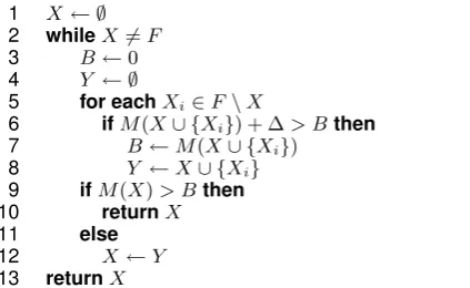
3 Feature Selection Algorithm
As in MaltOptimizer (Ballesteros and Nivre, 2014), our feature selection algorithm starts with a default feature set that is based on the MaltParser’s default feature model for an arc-standard parsing algorithm1, it first tests whether the features that are in the default model are actually useful, which means that whenever we remove any of the features of the default set, the accuracy is still the same (or better).
LetF={F1, . . . , Fn}be the full set of features,
letM(X)be the evaluation metric for feature setX, and let∆be the threshold.
1 X← ∅
2 whileX 6=F
3 B←0
4 Y ← ∅
5 for eachXi∈F\X
6 ifM(X∪ {Xi}) + ∆> Bthen
7 B←M(X∪ {Xi})
8 Y ←X∪ {Xi}
9 ifM(X)> Bthen
10 returnX
11 else
12 X←Y
[image:3.595.306.518.490.620.2]13 returnX
Figure 2: Algorithm for forward feature selection. After that, one by one, the algorithm tries to
add feature templates to the feature set. For each additional feature template a parser is trained for testing and if the accuracy is higher than the ac-curacy of the previous step plus a∆(threshold) then the feature in question is added to the fea-ture set. The selection process continues until all features have been tested, and therefore each feature has been either added or rejected. Most of the feature selection is based on the forward selection algorithm shown in Figure 2, although there is also a bit of backward selection from the default set.
The feature selection algorithm only has the training set as an input, and it splits it into train-ing and development to validate the outcomes of the experiments.2 After the feature selection, we
run the parser model on a held-out test set to measure its performance.
The feature selection is pruned following similar strategies to MaltOptimizer; there are features that are deeply related and the system tries to avoid unnecessary tests when some features happen to be excluded. For instance, the algorithm will not try to select the third position of the buffer for the part-of-speech, if the second position was excluded by the feature selection algorithm.
1http://www.maltparser.org/userguide.html
4 Experimental Set-Up
In order to set up the experiments for the feature selection algorithm, we carried out a series of tests based on the parser settings. From these experiments, we obtained the best parser settings, the threshold that provides the best results given a development set, and the best scoring method and some additional configurations, that gave us reliable results and a fast outcome.
We used the following corpora for our experiments. Chinese: We used the Penn Chinese Treebank 5.1 (CTB5), converted with the head-finding rules and conversion tools of Zhang and Clark (2008), with the same split as in (Zhang and Clark, 2008) and (Li et al., 2011).3 English: We used the WSJ section of the Penn Treebank, converted with the head-finding rules of Yamada and Matsumoto (2003) and the labeling rules of Nivre (2006).4 German:We used Tiger Treebank (Brants et al., 2002) in the improved dependency conversion by Seeker and Kuhn (2012). Hungarian: We used the Szeged Dependency Treebank (Farkas et al., 2012). Russian: We used the SynTagRus Treebank (Boguslavsky et al., 2000; Boguslavsky et al., 2002).
4.1 Parser settings
As outlined in Section 3, our feature selection experiments require the training of a large number of parsing models and applying these to the development set.5 Therefore, we aimed to find a training setup for the parser that provided fast training times while maintaining a realistic training and optimization scenario.
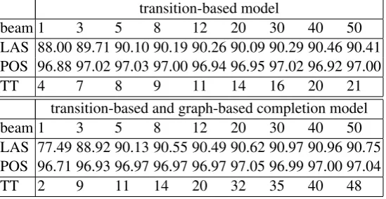
A major factor for the time usage is the beam size. The beam contains the alternative syntactic struc-tures that are considered in the parsing process, and thus it requires more time and memory while it normally provides better results. The parser uses two additional small beams to store the differently tagged syntactic structures and morphological structures, for the joint models. We explored a number of configurations and assessed the parsing performance by carrying out a set of experiments on the Penn Treebank and the training settings of Bohnet et al. (2013);6the results are shown in Table 1.
transition-based model
beam 1 3 5 8 12 20 30 40 50
LAS 88.00 89.71 90.10 90.19 90.26 90.09 90.29 90.46 90.41 POS 96.88 97.02 97.03 97.00 96.94 96.95 97.02 96.92 97.00
TT 4 7 8 9 11 14 16 20 21
transition-based and graph-based completion model
beam 1 3 5 8 12 20 30 40 50
LAS 77.49 88.92 90.13 90.55 90.49 90.62 90.97 90.96 90.75 POS 96.71 96.93 96.97 96.97 96.97 97.05 96.99 97.00 97.04
[image:4.595.163.438.422.564.2]TT 2 9 11 14 20 32 35 40 48
Table 1: Labeled Accuracy Score (LAS) in percent, Part-of-Speech tag accuracy POS in percent and training time (TT) in milliseconds per sentence. The parser was applied on the development set and trained over the Penn Treebank.
The table provides an overview of this preliminary experiment. The upper part of the table shows the performance when only using the transition-based model. The accuracy improvements are small when the beam-size becomes larger than 5. Even when we compared the results with the results of a beam size of 30, we observed only a small accuracy improvement. Further, we observe with a larger beam size a saturation where the accuracy does not improve and the parsing results show a small variance.
3Training: 001–815, 1001–1136. Development: 886–931, 1148–1151. Test: 816–885, 1137–1147. 4Training: 02-21. Development: 24. Test: 23.
5All this experiments were carried out on a CPU Intel Xeon 3.4 Ghz with 6 cores.
English German
∆ LAS UAS POS # LAS UAS POS MOR #
[image:5.595.125.475.62.201.2]0.05 90.17 91.39 97.00 40 90.57 92.81 97.89 90.45 41 0.02 90.24 91.52 97.04 54 90.83 93.00 98.01 90.55 49 0.01 90.17 91.45 96.90 54 90.90 92.95 97.98 90.69 60 0.00 90.43 91.71 97.00 57 90.89 92.98 97.94 90.59 68 -0.01 90.26 91.47 97.06 69 90.92 93.09 98.02 90.72 79 -0.02 90.27 91.52 97.05 77 91.27 93.37 98.17 90.84 93 -0.05 90.49 91.66 97.01 98 91.02 93.11 98.11 90.69 116 -∞ 90.37 91.65 96.98 188 90.77 93.00 98.14 89.56 188
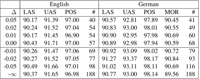
Figure 3: Accuracy scores depending on the threshold∆.
The feature selection starts with a default feature set that includes 20 features (cf. Section 3), and all these features are derived from the default feature models for MaltParser (Nivre et al., 2007)7. In total, the feature selection algorithm, for the transition-based model, may select 188 features. In Table 1 we show the training time (TT). We used this table to selected the optimal settings for the beam. After considering the trade-off between accuracy and speed, we selected for the feature selection a beam size of 8, since it obtains 90.19 LAS which is close to the highest accuracy score 90.46 and with this beam size the parser is fast. For a parser trained with all feature templates, the average parsing time per sentence is 9 milliseconds. With 20-60 features, we obtained a parsing time of 2-5 milliseconds per sentence, which is a faster and more optimal setting for the feature selection. Moreover, with a beam size of 40, we get parsing times that ranged depending on the number of features from 12 to 50 milliseconds per sentence, this is impracticable for feature selection experiments.
4.2 Selecting an Optimal Threshold
Feature templates are selected when they provide a higher accuracy compared to the previous feature set plus a threshold∆. To determine an optimal ∆for the feature selection, we carried out a series of experiments with different∆values. As a first step, we ran the feature selection algorithm starting from 0.05 and reducing the value stepwise to -0.05 (testing 0.05, 0.02, 0.01, 0.0, -0.01, -0.02, -0.05) with the intention of obtaining accuracy scores for all these settings. Table 3 shows the scores for our experiments on the development set for the English and German treebanks. We obtained an optimal trade-off between score and number of features with a∆of 0.0. With higher thresholds, such as 0.02 or 0.05, the feature selection algorithm was very restrictive, and resulted in lower accuracy scores. This indicates that there are several features that are not included that could contribute to a higher accuracy; for instance, in the German case, we see that the algorithm only selects 41 features. Moreover, the accuracy for English with a∆of 0.0 is even higher compared with the results obtained when all features were included (cf. last row:−∞). For German, we see a highest accuracy score with threshold of−0.02. We might get the best accuracy with this threshold when applied to the test set; however, the downside of this threshold is that the algorithm selected 25 more feature templates, which leads to a slower parser.
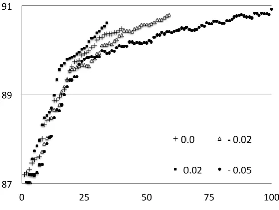
Figure 4 illustrates the accuracy gain depending on the number of features included. The development set of these graphs consist of 20% of the original training set. A negative∆leads to the inclusion of more features, which seem to provide even slightly higher results while including much more features. This outcome is not fully supported by the results from the development sets for English where we observed slightly lower results for a∆of -0.02 compared to 0.0.
To determine the optimal threshold∆for a language would come with a high computational cost, we carried out these experiments for English and German which show only small differences in accuracy in the threshold range around0. Therefore, we adopted0.0as threshold for our further experiments on other languages as well, cf. Table 4.
87 89 91
0 25 50 75 100
0.0 -‐ 0.02
[image:6.595.159.434.81.288.2]0.02 -‐ 0.05
Figure 4: Selected features (x-axis) vs Labeled Accuracy Score (y-axis). Features:transition-based
English German
LAS UAS POS # LAS UAS POS MOR # LAS 90.34 91.71 97.04 54 90.89 92.98 97.94 90.59 68
LUMP 90.38 91.57 97.09 55 90.82 92.88 98.11 90.65 53
PMLAS 90.12 91.38 97.02 40 89.27 91.66 98.0190.66 31
Table 2: Experiments with evaluation metrics with a ∆ of 0.0 on the development sets. Features:
transition-based. The morphology results are only shown for German, because the English treebank does not contain separate morphological features.
4.3 Selecting the Best Scoring Method
We carried out a number of experiments to determine the best criterion for the inclusion of features into the model. We tested several evaluation measures that compute the results of each model, that are LAS [labeled attachment score], LUMP8 [(labeled attachment score + unlabeled attachment score + mor-phology accuracy + part-of-speech accuracy)/4] and PMLAS9 [labeled attachment score, morphology accuracy and part-of-speech accuracy]. Table 2 shows the results of the feature selection for English and German for all these scoring methods. We finally selected LAS as our scoring method given that it pro-vides the best results for German and competitive results (at the same level) for English. LUMP is very similar, however, it seems a bit more restrictive than LAS. Moreover, PMLAS was the most restrictive measure, allowing only 31 features for German and 40 for English, which is the reason why there is a significant lower accuracy for the models selected with PMLAS.
Finally, it is worth mentioning that we explored an alternative criterion for the inclusion of features into the set. We explored the possibility to include only features that show a statistical significant im-provement. However, this criterion is too strict as only very few features showed a statistical significant improvement on its own.
4.4 Selection of Feature Templates of the Graph-based Completion Model
The graph-based completion model re-scores the beam incrementally and leads to a higher accuracy. We tried to select the graph-based feature templates of the completion model after the selection of the 8LMP [(labeled attachment score + morphology accuracy + part-of-speech accuracy)/3] would have been another alternative. However, we wanted to give the syntax still a higher weight in the feature selection process.
transition-based feature templates. This approach could not reach the accuracy gain shown by Bohnet and Kuhn (2012). We attempted to compensate this by starting the selection procedure from the default set with the intention of maximizing potential accuracy gains. However, this procedure did not lead to a better accuracy when later combined with the selected transition-based feature templates. We tried also to relax the threshold to -0.02 in order to include more features and to achieve a higher accuracy. Since this leads to better results, we performed the feature selection for the graph-based completion model with this setting.
4.5 Morphology for English
The Penn Treebank is annotated with part-of-speech tags that include morphological features such as
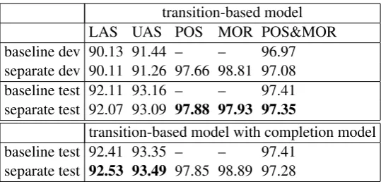
NNS(plural noun) orVBD(verb past tense). The corpus does not include separate morphological features. Splitting up these features could be useful because: (1) the parser might be able to generalize better when we use the word categories separated from morphological features, and (2) we might take advantage of the ability of the parser to predict morphology and part-of-speech based on the interaction with the syntax. Table 3 summarizes the results. Our transition-based parsing model shows only small differences between the scores for the original POS tag set and the tag set that separates the category and morphology.
transition-based model LAS UAS POS MOR POS&MOR baseline dev 90.13 91.44 – – 96.97 separate dev 90.11 91.26 97.66 98.81 97.08 baseline test 92.11 93.16 – – 97.41 separate test 92.07 93.09 97.88 97.93 97.35
transition-based model with completion model baseline test 92.41 93.35 – – 97.41
[image:7.595.164.434.287.416.2]separate test 92.53 93.49 97.85 98.89 97.28
Table 3: Experiments on Penn Treebank with separate representation of word category and morphology.
The results of the transition-based model, including the graph-based model shows some larger differ-ences
The labeled and unlabeled accuracy scores are not statistically significant and we concluded that (1) and (2) do not probably hold. Splitting up the morphology is a neutral operation in terms of labeled and unlabeled accuracy scores; however, it is worth noting that our results with the separate test for the completion model is more competitive, providing an improvement of 0.14 UAS.
5 Experiments: Feature Selection
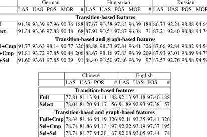
We applied the feature selection algorithm with the parameters determined in the previous sections on the corpora of Chinese, English, German, Hungarian and Russian, and we applied the outcome to parse the held-out test sets with a beam size of 40 and 25 training iterations. Table 4 shows the accuracy scores and the number of features selected for each language. The threshold for inclusion of the feature was set to0, cf. section 4.
The first row (Full) shows the accuracy scores for the full set of features, that includes all 188 feature templates of the transition-based feature set. The second row gives the accuracy scores that have been obtained with the reduced feature set gained by the feature selection algorithm described in Section 3.
German Hungarian Russian
LAS UAS POS MOR # LAS UAS POS MOR # LAS UAS POS MOR #
Transition-based features
Full 91.39 93.39 97.96 90.36 188 87.67 90.38 97.83 96.39 188 86.73 92.24 98.88 94.66 188
Select 91.34 93.36 97.88 90.48 68 87.94 90.51 97.87 96.38 71 87.21 92.40 98.88 94.74 64
Transition-based and graph-based features
Full+Cmp 91.77 93.63 98.14 90.77 326 88.88 91.33 97.84 96.41 326 87.66 92.84 98.82 94.56 326
Sel+Cmp 91.81 93.72 97.85 90.44 206 88.67 91.16 97.83 96.39 209 87.93 93.01 98.89 94.73 202
Sel+Sel 91.60 93.61 97.85 90.39 91 88.40 90.50 97.86 96.39 97 87.57 92.76 98.88 94.59 75
Chinese English
LAS UAS POS # LAS UAS POS #
Transition-based features
Full 77.81 81.13 94.11 188 92.13 93.18 97.40 188
Select 78.04 81.20 94.17 56 91.89 92.93 97.38 57
Transition-based and graph-based features Full+Cmp 78.34 81.46 94.19 326 92.41 93.35 97.41 326
Sel+Cmp 78.74 81.86 94.13 197 92.22 93.19 97.37 195
[image:8.595.90.503.65.337.2]Sel+Sel 78.74 81.77 94.28 67 92.08 93.05 97.44 74
Table 4: Labeled attachment score (LAS), unlabeled attachment score (UAS), part-of-speech accuracy (POS) and morphology accuracy (MOR) per language and model. The first two rows refer only to transition-based features while the last two rows include transition-based and graph-based features.Full
refers to a model with all transition-based features.Selectrefers to a model with selected transition-based features. Full+Cmp refers to a model with all transition-based features and all graph-based features.
Sel+Cmprefers to a model with selected transition-based features and all graph-based features.Sel+Sel
refers to a model with selected transition-based features and selected graph-based features. The English and Chinese accuracy scores exclude punctuation marks.
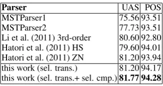
More about parsing time, training time and memory requirements is depicted in Section 6. A compar-ison with state of the art results as shown in the Tables 5a to 5d reveal that the parser with the selected features of the transition-based, and graph-based model are on an equal level for Chinese, Russian and Hungarian with state-of-the-art results. With the selected transition-based and the full graph-based fea-ture templates, the results for these languages surpass current state-of-the-art results.
6 Time and Memory Requirements
The number of feature templates has a serious impact on training time, parsing time and the amount of main memory required. The feature selection may have huge impact on the speed of a parser. Therefore, we measure the actual time and memory usage by applying the parser on the English test set of the Penn Treebank. This was done with different parsing models, and for each model, test runs were performed with an increasing number of CPU cores. Figure 6 shows an overview of the results.
The parsing model with all transition- and graph-based features takes on one CPU core 0.085 seconds per sentence (cf. Figure 6, line with rhombus). In contrast, the parser with selected transition-based features parses a sentence in less than half of the time (0.042 seconds, line with crosses). The parsing accuracy is only 0.42 percentage points worse (93.35 vs. 92.93 UAS). When we compare the first parsing model with the model with selected transition-based and graph-based features, we observe a parsing time of 0.066 seconds per sentence and a small accuracy difference of only 0.27.
Parser UAS LAS POS McDonald et al. (2005a) 90.9
McDonald and Pereira (2006) 91.5 Huang and Sagae (2010) 92.1 Koo and Collins (2010) 93.04 Zhang and Nivre (2011) 92.9 Martins et al. (2010) 93.26
Bohnet and Nivre (2012) 93.38 92.44 97.33 this work (sel. trans.& sel. cmpl.) 93.05 92.0897.44
this work (P&M cf. Table 3) 93.49 92.53 – Koo et al. (2008)† 93.16
Carreras et al. (2008)† 93.5 Suzuki et al. (2009)† 93.79
(a) Accuracy scores for WSJ-PTB. Results marked with†use additional information sources and are not directly comparable to the others.
Parser UAS POS
MSTParser1 75.56 93.51
MSTParser2 77.73 93.51
Li et al. (2011) 3rd-order 80.60 92.80 Hatori et al. (2011) HS 79.60 94.01 Hatori et al. (2011) ZN 81.20 93.94 this work (sel. trans.) 81.20 94.17 this work (sel. trans.+ sel. cmp.)81.77 94.28
(b) Accuracy scores for the Chinese treebank converted with the head rules of Zhang and Clark (2008). MSTParser results from Li et al. (2011). UAS scores from Li et al. (2011) and Ha-tori et al. (2011) recalculated from the separate accuracy scores for root words and non-root words.
Parser UAS LAS POS
Farkas et al. (2012) 90.1 87.2 Bohnet et al. (2013) 91.3 88.9 98.1
this work (sel. trans. & sel. cmpl.) 90.50 88.40 97.83 this work (sel. trans. & full cmpl.) 91.16 88.67 97.86 (c) State of the art comparison for Hungarian. The table shows that we can reach state of the art performance with less features.
Parser UAS LAS POS
Boguslavsky et al. (2011) 90.0 86.0 Bohnet et al. (2013) 92.8 87.6 98.5 this work (sel. trans. & sel. cmp.) 92.76 87.5798.89
[image:9.595.332.496.60.146.2]this work (sel. trans. & full cmp.)93.01 87.9398.88 (d) State of the art comparison for Russian.
Figure 5: Comparison with state of the art results.
0 0,025 0,05 0,075 0,1
1 2 3 4 5 6
se
conds
CPU Cores
(1) all graph & tr. features (2) selected tr. & all. graph features (3) selected graph & tr. features (4 )selected tr. features
id trans. features graph features # features UAS
(1) all all 75.8 M 93.35
(2) selected all 43.5 M 93.22
(3) selected selected 22.1 M 93.08 (4) selected none 17.8 M 92.93
Figure 6: Parsing Time in relation to CPU cores and number of features in the hash kernel in millions.
demonstrate that we can double the parsing speed and maintain a very high parsing accuracy.
7 Conclusions
In this paper, we have presented the first feature selection algorithm for agenda-based dependency pars-ing. Our algorithm could be directly used out of the box,10and applied to a new data set or language to get an optimized feature model for a agenda-based parser such as the Mate tools.11
Our feature selection algorithm provides models with even higher accuracy for Chinese and Russian, cf.Table 4. For the remaining languages the models provide accuracy scores that are comparable to the ones obtained by models including a larger set of feature templates. For all languages, the feature models gained via feature selection are faster and require less memory, which make them very useful for practical applications. We conclude that feature models obtained with the feature selection algorithm 10The source code and the feature models found for each language are available athttps://code.google.com/p/ mate-tools/
[image:9.595.91.283.63.197.2]often provide a comparable accuracy level while they are considerable faster. Finally, our model for English with the separated morphology tag-set provides one of the best results reported with93.49UAS. Additionally, the feature selection algorithms for this setting shows competitive results with a largely reduced number of feature templates, and thus less parsing time and lower memory requirements. The parser is faster (almost double) and provides93.05UAS which is also among the best results.
Acknowledgments
This research project was supported by funding of the European Union (PCIG13-GA-2013-618143).
References
Eneko Agirre, Kepa Bengoetxea, Koldo Gojenola, and Joakim Nivre. 2011. Improving Dependency Parsing with Semantic Classes. InThe 49th Annual Meeting of the Association for Computational Linguistics: Human Language Technologies (ACL), pages 699–703, Portland, USA.
Miguel Ballesteros and Joakim Nivre. 2014. MaltOptimizer: Fast and Effective Parser Optimization. Natural Language Engineering.
Miguel Ballesteros. 2013. Effective morphological feature selection with MaltOptimizer at the SPMRL 2013 shared task. InProceedings of the Fourth Workshop on Statistical Parsing of Morphologically-Rich Languages, pages 53–60.
Igor Boguslavsky, Svetlana Grigorieva, Nikolai Grigoriev, Leonid Kreidlin, and Nadezhda Frid. 2000. Depen-dency treebank for Russian: Concept, tools, types of information. In Proceedings of the 18th International Conference on Computational Linguistics (COLING), pages 987–991.
Igor Boguslavsky, Ivan Chardin, Svetlana Grigorieva, Nikolai Grigoriev, Leonid Iomdin, Leonid Kreidlin, and Nadezhda Frid. 2002. Development of a dependency treebank for Russian and its possible applications in NLP. In Proceedings of the 3rd International Conference on Language Resources and Evaluation (LREC), pages 852–856.
Igor Boguslavsky, Leonid Iomdin, Victor Sizov, Leonid Tsinman, and Vadim Petrochenkov. 2011. Rule-based dependency parser refined by empirical and corpus statistics. InProceedings of the International Conference on Dependency Linguistics, pages 318–327.
Bernd Bohnet and Jonas Kuhn. 2012. The best of bothworlds - a graph-based completion model for transition-based parsers. InProceedings of the 15th Conference of the European Chapter of the Association for Computa-tional Linguistics (EACL), pages 77–87.
Bernd Bohnet and Joakim Nivre. 2012. A transition-based system for joint part-of-speech tagging and labeled non-projective dependency parsing. In Proceedings of the 2012 Joint Conference on Empirical Methods in Natural Language Processing and Computational Natural Language Learning, pages 1455–1465, Jeju Island, Korea, July. Association for Computational Linguistics.
Bernd Bohnet, Joakim Nivre, Igor Boguslavsky, Rich´ard Farkas, Filip Ginter, and Jan Hajic. 2013. Joint morpho-logical and syntactic analysis for richly inflected languages. Transactions of the Association for Computational Linguistics(TACL), 1:415–428.
Sabine Brants, Stefanie Dipper, Silvia Hansen, Wolfgang Lezius, and George Smith. 2002. TIGER treebank. In
Proceedings of the 1st Workshop on Treebanks and Linguistic Theories (TLT), pages 24–42.
Xavier Carreras, Michael Collins, and Terry Koo. 2008. Tag, dynamic programming, and the perceptron for efficient, feature-rich parsing. InProceedings of the Twelfth Conference on Computational Natural Language Learning (CoNLL), pages 9–16.
Xavier Carreras. 2007. Experiments with a higher-order projective dependency parser. InProceedings of the CoNLL Shared Task at the 2007 Joint Conference on Empirical Methods in Natural Language Processing and Computational Natural Language Learning (EMNLP-CONLL), pages 957–961.
Rich´ard Farkas, Veronika Vincze, and Helmut Schmid. 2012. Dependency parsing of hungarian: Baseline re-sults and challenges. InProceedings of the 15th Conference of the European Chapter of the Association for Computational Linguistics (EACL), pages 55–65.
Johan Hall, Jens Nilsson, Joakim Nivre, G¨ulsen Eryi˘git, Be´ata Megyesi, Mattias Nilsson, and Markus Saers. 2007. Single Malt or Blended? A Study in Multilingual Parser Optimization. InProceedings of the CoNLL Shared Task at the 2007 Joint Conference on Empirical Methods in Natural Language Processing and Computational Natural Language Learning (EMNLP-CONLL), pages 933–939.
Johan Hall. 2008. Transition-Based Natural Language Parsing with Dependency and Constituency Representa-tions. Ph.D. thesis, V¨axj¨o University.
Jun Hatori, Takuya Matsuzaki, Yusuke Miyao, and Jun’ichi Tsujii. 2011. Incremental joint pos tagging and dependency parsing in chinese. pages 1216–1224.
He He, Hal Daum´e III, and Jason Eisner. 2013. Dynamic feature selection for dependency parsing. InEMNLP, pages 1455–1464.
Liang Huang and Kenji Sagae. 2010. Dynamic programming for linear-time incremental parsing. InProceedings of the 48th Annual Meeting of the Association for Computational Linguistics (ACL), pages 1077–1086. Terry Koo and Michael Collins. 2010. Efficient third-order dependency parsers. InProceedings of the 48th Annual
Meeting of the Association for Computational Linguistics (ACL), pages 1–11.
Terry Koo, Xavier Carreras, and Michael Collins. 2008. Simple semi-supervised dependency parsing. In Pro-ceedings of the 46th Annual Meeting of the Association for Computational Linguistics (ACL), pages 595–603. Zhenghua Li, Min Zhang, Wanxiang Che, Ting Liu, Wenliang Chen, and Haizhou Li. 2011. Joint models for
chinese POS tagging and dependency parsing. In Proceedings of the Conference on Empirical Methods in Natural Language Processing (EMNLP), pages 1180–1191.
Andre Martins, Noah Smith, Eric Xing, Pedro Aguiar, and Mario Figueiredo. 2010. Turbo parsers: Dependency parsing by approximate variational inference. InProceedings of the Conference on Empirical Methods in Nat-ural Language Processing (EMNLP), pages 34–44.
Ryan McDonald and Fernando Pereira. 2006. Online learning of approximate dependency parsing algorithms. In
Proceedings of the 11th Conference of the European Chapter of the Association for Computational Linguistics (EACL), pages 81–88.
Ryan McDonald, Koby Crammer, and Fernando Pereira. 2005a. Online large-margin training of dependency parsers. InProceedings of the 43rd Annual Meeting of the Association for Computational Linguistics (ACL), pages 91–98.
Ryan McDonald, Fernando Pereira, Kiril Ribarov, and Jan Hajiˇc. 2005b. Non-projective dependency parsing using spanning tree algorithms. InProceedings of the Human Language Technology Conference and the Conference on Empirical Methods in Natural Language Processing (HLT/EMNLP), pages 523–530.
Peter Nilsson and Pierre Nugues. 2010. Automatic Discovery of Feature Sets for Dependency Parsing. In Pro-ceedings of the 23rd International Conference on Computational Linguistics (COLING), pages 824–832. Joakim Nivre and Johan Hall. 2010. A quick guide to MaltParser optimization. Technical report, maltparser.org. Joakim Nivre, Johan Hall, Jens Nilsson, G¨ulsen Eryi˘git, and Svetoslav Marinov. 2006. Labeled pseudo-projective
dependency parsing with support vector machines. InProceedings of the 10th Conference on Computational Natural Language Learning (CoNLL), pages 221–225.
Joakim Nivre, Johan Hall, Jens Nilsson, Atanas Chanev, G¨uls¸en Eryiˇgit, Sandra K¨ubler, Svetoslav Marinov, and Erwin Marsi. 2007. Maltparser: A language-independent system for data-driven dependency parsing. Natural Language Engineering, 13:95–135.
Joakim Nivre. 2006. Inductive Dependency Parsing. Springer.
Wolfgang Seeker and Jonas Kuhn. 2012. Making ellipses explicit in dependency conversion for a german treebank. pages 3132–3139.
Jun Suzuki, Hideki Isozaki, Xavier Carreras, and Michael Collins. 2009. An empirical study of semi-supervised structured conditional models for dependency parsing. InProceedings of the Conference on Empirical Methods in Natural Language Processing (EMNLP), pages 551–560.
Hiroyasu Yamada and Yuji Matsumoto. 2003. Statistical dependency analysis with support vector machines. In
Proceedings of the 8th International Workshop on Parsing Technologies (IWPT), pages 195–206.
Yue Zhang and Stephen Clark. 2008. A tale of two parsers: Investigating and combining graph-based and transition-based dependency parsing. InProceedings of the Conference on Empirical Methods in Natural Lan-guage Processing (EMNLP), pages 562–571.