Learning Succinct Models: Pipelined Compression with L1 Regularization, Hashing, Elias Fano Indices, and Quantization

Learning Succinct Models: Pipelined Compression with

L1-Regularization, Hashing, Elias–Fano Indices, and Quantization

Hajime Senuma† ‡ _{and Akiko Aizawa}‡ † †_{University of Tokyo, Tokyo, Japan} ‡_{National Institute of Informatics, Tokyo, Japan}

{senuma,aizawa}@nii.ac.jp

Abstract

The recent proliferation of smart devices necessitates methods to learn small-sized models. This paper demonstrates that if there aremfeatures in total but onlyn=o(√m)features are required to distinguish examples, withΩ(logm)training examples and reasonable settings, it is possible to obtain a good model in asuccinctrepresentation usingnlog₂ m_n+o(m)bits, by using a pipeline of existing compression methods: L1-regularized logistic regression, feature hashing, Elias–Fano indices, and randomized quantization. An experiment shows that a noun phrase chunking task for which an existing library requires 27 megabytes can be compressed to less than 13 kilobytes without notable loss of accuracy.

1 Introduction

The age of smart devices has arrived. Cisco reports that, as of 2015, smartphones and tablets account for 15% of IP traffic (against 53% for PCs), and further predicts that, by 2020, this share will have grown to 43%, surpassing the 29% of PCs (Cisco Systems, 2016). This trend increases the need for intelligent processing for these platforms. Hence, the study of statistical methods for natural language process-ing (NLP) systems on mobile devices has received considerable attention in recent years (Ganchev and Dredze, 2008; Hagiwara and Sekine, 2014; Chen et al., 2015).

Among the various issues in this setting, storage costs pose a particular challenge, because the size of the resulting models often grow quickly. Even a simple noun phrase (NP) chunker can easily take dozens of megabytes if na¨ıvely implemented. Suppose we have m features. A direct implementation then consumesZ(A) +O(mζ), whereZ(A)represents the size of analphabetA, or afeature dictionarythat maps a feature string to an index into its parameter vector, andO(mζ)represents the space complexity of a dense real vector as the parameter where usingζ bits to achieve a certain amount of float precision (64m if using double-precision floats). These large-sized models are not only inefficient in terms of network bandwidth, but also significantly increase energy consumption (Han et al., 2016). Therefore, it is vital to devise a method that achieves as small a model as possible.

One of the basic properties of information theory says that, to represent a set of n non-negative integers less than m (or, equivalently, a bit vector of size m containing n 1s), we need at least

Bm,n = ⌈log2(mn

)

⌉ ≈ nlog₂m

n bits. Recent studies in theoretical computer science show that it is

possible to compress a set of non-negative integers while keeping some primitive operations under suc-cinctrepresentations, that is, data structures using onlyBm,n+o(m)bits.

As an analogy to succinct data structures, one may ask a question: if there aremfeatures, but onlyn

of these are useful for distinguishing data, how many bits are required to obtain a good classifier? This paper shows that under several reasonable assumptions such asn=o(√m), withΩ(logm)examples, it is possible to obtain a model that performs similarly to the original classifier, by using onlyBm,n+o(m)

bits.

To evaluate our method, we implemented conditional random fields (CRFs) by using our pipelined architecture and conducted an experiment on an NP chunking model. The results show that 27 megabytes can be reduced to about 13 kilobytes.

This work is licensed under a Creative Commons Attribution 4.0 International Licence. Licence details: http:// creativecommons.org/licenses/by/4.0/

In summary, our work is significant in that

1. we present a pipelined method to acquire asuccinctmodel that also has almost the same predictive performance as the model of Ng (2004),

2. although the above method is achieved under some conditions and penalties, the conditions are not ungrounded for NLP tasks and the the penalties are neglible for largem,

3. we also introduce a bitwise trick to perform fast unbiased feature hashing, a part of the pipeline,

4. and our experimentations on sequential labeling tasks achieve smaller models than existing libraries by a factor of one thousand, demonstrating the high practical value of our approach.

This paper is organized as follows. In Section 2, we mention related work. In Section 3, we explain the notation used in the paper. In Section 4, we introduce and analyze our methods. In Section 5, we evaluate our approach by an experiment.

2 Related Work

Ganchev and Dredze (2008) were one of the earliest groups to recognize the importance of acquir-ing small models for mobile platforms. They also showed that na¨ıve hashacquir-ing tricks for features (now commonly known asfeature hashing) can greatly improve the memory efficiency without much loss of accuracy. Shi et al. (2009) showed that feature hashing could be applied to graph models. Weinberger et al. (2009) proposed an unbiased version of feature hashing. Bohnet (2010) applied the method to dependency parsing, and found that it improves not only memory efficiency, but also speed performance. Recent studies (Chen et al., 2015) suggest that hashing tricks also work well in deep neural networks too. Feature selection through the L1 regularization is also known to be effective, since, roughly speaking, the number of features in the final model results in being logarithmic to the number of total features (Ng, 2004). Online optimization (vis-´a-vis batch optimization) with the L1-regularization term gained atten-tion from around 2010 (Duchi and Singer, 2009; Tsuruoka et al., 2009), and with the AdaGrad (Duchi et al., 2011) method becoming particularly popular, because of its theoretical and practical performance.

Compression by quantization is closely related to machine learning. For eaxmple, the Lloyd quan-tization (Lloyd, 1982) is now used as a popular clustering method known as the K-means clustering. Golovin et al. (2013) showed that simple (simplistic, in fact) quantization techniques actually exhibit good performance in common settings used in NLP; although their methods themselves were basic, they analyzed theoretical effects in detail, and these serve as the key ingredients for our error analysis in Section 4.

The compression of indices is a classical topic in information retrieval (IR). Vigna (2013) introduced the Elias–Fano structure (Fano, 1971; Elias, 1974) into IR, although this was alreadly a popular theme in the succinct data structures community (Grossi and Vitter, 2005; Okanohara and Sadakane, 2007; Golynski et al., 2014). Although other types of succinct structures are common in NLP as well (Watanabe et al., 2009; Sorensen and Allauzen, 2011; Shareghi et al., 2015), the Elias–Fano structure is in that, if regarded as a binary vector, the order of compression ratio depends on the number of 1s (rather than the total length of a vector) and achieves better compression ratio than other succinct models for binary vectors if the ratio of 1s is very low (empirically, below 10%); to put it more concretely, the structure is very attractive when unnecessary indices are culled by some techniques such as L1-regularization. Because of its simplicity and compression ratio, the Elias–Fano structure even gained a certain degree of popularity in industry; for example, as of 2013, it is used as one of the backbones of Facebook’s social graph engine (Curtiss et al., 2013). Several variants have been proposed, including sdarry (Okanohara and Sadakane, 2007) and the partitioned Elias–Fano indices (Ottaviano and Venturini, 2014).

Han et al. (2015)’s three-step pruning process, Han et al. (2016) gained great empirical success using deep compression, or pipelined compression for a deep neural network with pruning, trained quantization, and Huffman coding.

3 Notation

The base of logarithm iseif not stated explicitly. If the base isx(x ̸=e), we writelog_x. Edenotes an expectation,Rdenotes a set of real values, andNdenotes a set of non-negative integers. δi,j represents

the Kronecker’s delta, that is, δi,j = 1if i = j, and 0 otherwise. Bm,n represents the

information-theoretic lower bound of encoding a bit vector of sizemwithn1s, that is,n⌈log₂(m_n)⌉.

4 Learning Succinct Models

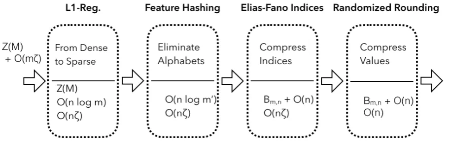
Figure 1: Overview of pipelined compression.

In this section, we present a supervised learning method to obtain a small-sized model for classification tasks. For simplicity, we assume binary classification for each labely ∈ {0,1} by logistic regression. Suppose there is a set ofmfeatures and a datasetT ={(x(0)_{, y}(0)_),(x(1)_{, y}(1)_{, ...,(x}(T−1)_{, y}(T−1)₎}_of

T training examples drawn i.i.d. from some distributionD.

Consider the following optimization problem with the L1-regularization termR(θ) =||θ||1

max

θ

T_∑−1

i=0

logp(yi |xi;θ)

subject to R(θ)≤B.

(1)

Our goal is to obtain a good parameterθthat minimizes the expected logistic log loss, that is,

ε(θ) =E_(x,y)∼D[−logp(y|x;θ)] (2)

with as small a model as possible. We also define the empirical loss

ˆ

ε(θ) = ˆεT(θ) = _T1

T_∑−1

i=0

−logp(yi |xi;θ). (3)

Them-dimensional vectorθis often implemented as a float array of sizem, consumingO(mζ)bits. Concretely, it occupies64mbits if we use double-precision (ζ = 64) and32mbits if single-precision (ζ = 32). As m can be millions, billions, or more in NLP tasks, this size complexity is often non-negligible for mobile and embedded devices (e.g., 762.9 megabytes for 100,000,000 features when using double-precision).

represents “the current token isappropriate, the previous token isI, and the current label isVERB”, one possible formulation is f12 = utf8("bigram[-1:0]=I:appropriate&label=VERB"), whereutf8denotes a non-negative integer given by the UTF-8 bit representation of a string. A weight value for this feature can then be accessed asθ_A(f12). There are two problems with the use of alphabets. First, they consume too much storage space (Ganchev and Dredze, 2008). Second, if implemented with a hash table (as is often the case), they are so slow that they become the bottleneck of the entire learning system (Bohnet, 2010). In the following,Z(A)denotes the size of an alphabetA.

4.1 Pipelined method

Let us now introduce a pipelined method to reduce bothO(mζ)andZ(A).

Definition 4.1. Given inputsT,

1. Train the model by using L1-regularization according to the method of Ng (2004):

(a) Divide the dataT into a training setT1of the size(1−γ)T and a development setT2 of the sizeγT, for someγ ∈R.

(b) ForB = 0,1,2,4, ..., C, solve the optimization under each of these hyperparameters withT1, givingθ0, ...,θC.

(c) Chooseθ= arg min_{{i∈0,1,2,...,C}}εˆT2(θi), or the best model for the development data set.

As we performed the L1-regularization, it is safe to assume that the non-zero components are quite small.Z(A) +O(nlogm) +O(nζ);Z(A)for the alphabet,⌈logm⌉bits for each of thenindices, andzeta) bits for each of thenvalues.

2. Eliminate the alphabet and reduce the dimensionality of vectors by using theunbiased feature hash-ing(Weinberger et al., 2009). Given two hash functions h: N → {0, ..., m′ _{−1} and ξ:N →} {−1,1}, we define the (unbiased)hashed feature map ϕsuch thatϕ(h,ξ)(x) ₌ ∑

j:h(j)=iξ(i)xi.

We apply thisϕto the parameter vector and all future input vectors. As this map acts as a proxy for the alphabet, we no longer need to store the alphabet. As a side-effect, if we choosem′ _{< m,} the dimensionality is reduced fromm tom′_{. Note that this is said to be unbiased because given} ⟨x,x′_{⟩ϕ :=} ⟨_ϕ(h,ξ)_{(x), ϕ}(h,ξ)_(x′₎⟩_{, E⟨x,x}′_{⟩ϕ = ⟨x,x}′_{⟩. In other words, on average, prediction} using a hashed map space is the same as the original version.

At this point, the size has been reduced toO(nlogm′_{) +O(nζ);⌈logm}′_{⌉for each of thenindices} andζ) bits for each of thenvalues.

3. Compress the set ofnindices by using the Elias–Fano scheme (Fano, 1971; Elias, 1974). In brief,

nintegers are compressed ton⌈log₂m/n⌉+f(n), wheref(n) =O(n)andf(n)≤2Snfor some speed-memory trade-off hyperparameter1 ≤ S <2 (usually less than1.01). We omit the details here, but interested readers may consult Vigna (2013)’s good introduction.

At this point, the size has been reduced ton⌈log₂m′_{/n⌉+O(n) +O(nζ).}

4. Compress the set of values by using theunbiased randomized rounding(Golovin et al., 2013). Let

µandν be some non-negative integers, then it encodes each value as a fixed-point number with Qµ.ν encoding, that is, asµinteger bits andν fractional bits (e.g., ifµ=ν = 2, we can represent a maximum of(11.11)2 = 3.75). Including a sign bit,µ+ν+ 1for each value.µandν are chosen so that they satisfy the conditions of the error anaysis in the following subsection.

At this point, the size has been reduced ton⌈log₂m′_/n⌉+O(n).

Overall, becausen⌈log₂m/n⌉=Bm,n+O(n)(Golynski et al., 2014), choosingm′ < mand assuming n = o(m) achieves a model with Bm,n +o(m). In the next subsection, however, we assume tighter

4.2 Error analysis

Each compression technique (except Elias–Fano) adds several penalties to the predictive performance. Therefore, intuitively, pipelined compression should lower the performance significantly. Contrary to such intuition, however, the increase in the error is negligible under certain circumstances.

Theorem 4.2. Suppose that there existmfeatures in total, but onlynfeatures are important, so that the optimal parameter vectorθ∗ _∈Rm_{has onlynnon-zero components with indices0≤i0, i1, ..., in−1 <} m. Further, assume that each non-zero component is bounded by some constant no less than1, that is,

0<|θij| ≤Kforj= 0, ..., n−1withK ≥1.

Let us be given a training data setT ={(x(0)_{, y}(0)_),(x(1)_{, y}(1)_{, ...,(x}(T−1)_{, y}(T−1)₎}_{ofT training}

examples drawn i.i.d. from some distribution D. Assume that the number of non-zero components of each input is always bounded by some non-negative constant much smaller thanm, and thatnis also much smaller thanmas follows:

||x||0 ≤kfor any(x, y)∼ D, k≥0, k=o(√m), n=o(√m), andK=o(m). (4)

Then, with probability at least (1−δ)(1 +f1(m))where f1(m) = o(1), it is possible to obtain a

model with size (in bits) at most

Bm,n+o(m) (5)

with errors to the expected logistic loss

ε(ˆθ)≤ϵmul(ε(θ∗) +ϵadd) (6)

whereϵmul = 1 +f2(m)withf2 such thatf2(m) = o(1), by performingC ≥ nk iterations to find a

good hyperparameter and by using theT examples such that

T = Ω((logm)·poly(n, K,log(1/δ),1/ϵadd, C)). (7)

Prior to its proof, let us explain what the above theorem says. If we omit the conditions of Equation (4), we have the same setting used in Ng (2004, Theorem 3.1). Thus, if we perform L1-regularized learning as defined in 1 of Definition 4.1, Ng’s theorem implies that Equations (6) and (7) hold, satisfyingf1(m) = 0 andf2(m) = 0.

In other words, the above theorem implies that if we add the conditions defined in Equation (4)) to Ng’s theorem, it is possible to obtain a succinct representation (Equation (5)) whose predictive performance is nearly as good as that of Ng’s theorem, albeit with a probabilistic penaltyf1(m)and an error penalty

f2(m). However, the penalties are negligible becausef1(m) =o(1)andf2(m) =o(1).

Note that for NLP tasks, some of the conditions can be justified to a certain extent by the power law. Let us follow the discussion presented by Duchi et al. (2011, Section 1.3). In NLP tasks, the appearance of features often follows the power law. Thus, we can assume that thei-th most frequent feature appears with probabilitypi = min(1, ci−α)for some a ∈ (1,+∞) and a positive constantc.

Givenx,E||x||0 ≤c∑_im₌₁i−α/2 _{=O(logd)forα≥2and||x||0 ≤O(m}1−α/2_{)forα ∈(1,2). Thus}

E||x||0 = o(√m) for anyxandα ∈ (1,+∞). This assumption and derivation by Duchi et al. imply that the conditionk=o(√m)is not ungrounded. The same discussion applies ton=o(√m)too. The conditionK =o(m)is less obvious than the other two, but we often assume a good parameter does not have any excessively large values.

We now prove the above theorem.

Proof. If we omit the conditions of Equation (4)), then the method in 4.1.1 can be used to show that Equations (6) and (7) hold, satisfyingϵmul = 1(Ng, 2004, Theorem 3.1).

analysis of randomized rounding requires the absolute value of any index to be bounded by1. Hence, applying feature hashing before randomized rounding can break the subsequent analysis. Thankfully, if we useh : N → 0, ..., m′ _{such that||x||0 = o(m}′_{) for any x ∈ D, with high probability(that is,}

1−o(1)), collisions never occur. This is a well-known fact resulting from Sterling’s approximation (in the following ,f, g, h, iareo(1)and irrelevant to the rest of this proof).

(

n k

)

= _k!(nn!_−k)! = (1 +f(n))

√

2πne−n_nn

k!(1 +g(n−k))√2π(n−k)e−(n−k)_(n−k)n−k

= _{(1 +}(1 +_g(nf(n))_−k))·_k!1 · (

n n−k

)_1/2

e−k

(

n n−k

)_−k(

n n−k

)_n

nk

= _{(1 +}(1 +_g(nf(n))_−k))·n_k!k · (

1−k_n )_k−1/2

e−k

(

1−k_n )_−n

= _{(1 +}(1 +_g(nf(n))_−k))·n_k!k ·(1 +o(1))e−k( 1

1− k n

)n

= _{(1 +}(1 +_g(nf(n))(1 +_{−k))(1 +}h(k))_i(n))·n_k!k ·e−k_· 1 e−k =

(1 +f(n))(1 +h(k)) (1 +g(n−k))(1 +i(n))·

nk k!

Using this equation, it is possible to estimate the hash collision ratio. If we assume Equation (4),

m′ _=c√_{mfor some positivecsatisfies the condition we mentioned above.}

We then apply the Elias–Fano structure defined in Definition 4.1.3. Because this is a lossless compres-sion method for indices, the error analysis remains the same. The remaining problem is how to store the values ino(m)bits.

Finally, we apply the unbiased randomized rounding as in Definition 4.1.4. Golovin et al. (2013, Theorem 4.3) implies that if the value of each non-zero component of θ∗ _{is bounded by some K and} the number of non-zero components of any input is bounded by somek such thatK ≥ 1 andk ≥ 0, then it is possible to derive a new parameter vectorθˆ, with each value using(1 +µ+ν)bits, such that

ε(ˆθ)≤ϵmul·ε(θ∗), where

0≤ϵmul ≤2χ√2πkexp

(

χ2_n

2

)

, (8)

µ = ⌈log₂K⌉(= o(logm)ifK = o(m)), andν = −log₂χ (soχ = 1

2ν). If we use ν =⌈cm1/2⌉(= Θ(√m))for some positive constant c, assuming the conditions (4) hold, ϵmul = f2(m)with f2 such that f2(m) = o(1). Here f2(m) = o(1) holds because limm→+∞χ√k = limm→+∞√k·χ2 =

limm→+∞ √

o(√m)/O(2m1/2_{) = 0and the same limit also applies to theχ2nterm.}

Thus, to store the values, we needn(1 +µ+ν) = o(√m)·(1 +o(logm) + Θ(√m)) =o(m)bits in total. This completes the proof.

4.3 Practical settings

In practical situations, several violations of the method can make it more efficient.

Another issue involves solving Equation (1). Several concrete optimization algorithms such as AdaGrad (Duchi et al., 2011) solve the dual problem of Equation (1), that is,

arg maxθ ∑_T−1

i=0 logp(yi|xi;θ)−λR(θ)whereλ∝ B1 forB > 0. This is said to be dual because, for

anyθobtained by Equation (1) with some hyperparameterB, there is exactly one hyperparameterλthat gives the sameθ. Unfortunately, it is often impossible to get the exact relationship between the hyperpa-rametersB andλ. However, becauseλ∝ _B1, a good value may be found by tryingλ= 1,1₂,1₄,1₈, ....

4.4 Bitwise feature hashing

On first examination, unbiased feature hashing (Weinberger et al., 2009) may appear to be twice as costly as the na¨ıve version (that is, alwaysξ(i) = 1in Definition 4.1.2), as it requires two hash functions to be computed: h and ξ. Actually, by leveraging some bitwise operations, we need only one hash computation and just another three CPU cycles per feature to perform the unbiased version. Let us consider the following algorithm to convertkitems of an original index–value pair to the same number of items of pairs under feature hashing. In the algorithm, >> denotes an arithmetic right shift (also called a signed right shift).

Data: A 2-tuple of indices and values(I;V)such thatI ∈Nk_{andV ∈R}k_{for somek.}

Dimensionalitym′_satisfyingm′ _{= 2}a_{for somea∈N.}

Result: A 2-tuple of indices and values(I∗_;V∗_{)such thatI}∗ _∈Nk_andV∗ _∈Rk_{for somekand} 0≤i′ _{< m}′_<232_{for anyi∈I}∗_.

1 MASK ←m′−1;

2 forinti= 0;i < k;i←i+ 1do 3 t←h(I_i);

4 sign←(t >> 31)|1; 5 I_i∗ ←t & MASK; 6 V_i∗←sign·V_i; 7 end

8 return(I∗;V∗);

Algorithm 1:Bitwise unbiased feature hashing

The improvements over the original version are:

1. the original version requires two hash functions, whereas our version requires only one,

2. the resulting index–value pairs are not merged—because the dot-product between two vectors is distributive (a·(b+c) =a·b+a·c), there is no need to merge indices—so there is no need to use slow data structures such as hash maps for merging, and

3. compared with Bohnet (2010)’s approach, which uses a% (modulo) operator to gain the desired dimension, our approach uses & (bitwise mask), so it runs faster in common architectures. The downside is that the resulting dimension will be limited to a power of two.

5 Experimental Results

To evaluate our approach, we implemented a linear-chained conditional random field (CRF) (Lafferty et al., 2001; Sha and Pereira, 2003) and tested it on an NP chunking task. For the optimization problem, we used the AdaGrad, an online optimization algorithm, with the L1-regularization term by diagonal primal-dual subgradient update (Duchi et al., 2011).

5.1 Implementation

We implemented our CRF library with ECMAScript 6, but its core component for optimization computa-tion was handwritten by asm.js1_{, a subset of ECMAScript 6 (that is, so-called JavaScript 6). The language}

was designed mainly by Mozilla as a performance improvement technique for web platforms. Although it is conformant to ECMAScript 6, the language is actually lower-level than C, and Mozilla claims it is only at most twice as slow as native code. We used the language because, by using a JavaScript-compatible language, it is possible to embed the resulting classifier in web pages for use as a fundamental library in web systems, not only on desktop machines but also on mobile platforms.

5.2 NP chunking

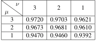
µ ν 3 2 1

3 0.9720 0.9703 0.9621 2 0.9673 0.9681 0.9610 1 0.9470 0.9460 0.9392

Table 1: Macro-averaged F1 values under variousµandνvalues forQµ.νencoding.

To test our CRF implementation, following Sha and Pereira (2003), we performed an NP chunking task using the CoNLL-2000 text chunking task data (Tjong Kim Sang and Buchholz, 2000). In the shared task data, the labels B-NP and I-NP were retained, but all other labels were converted to O. Therefore, this is basically a sequential labeling problem with three labels. The features are the same as those used by Sha and Pereira (2003), except that they reformulated two consecutive labels as a new one, whereas we used the original labels. The total number of features is 1,015,621.

The training dataset consists of 8,936 instances, and the test dataset contains 2,012. Of the training data set, we used 7,148 instances (4/5) for training and the remaining 1,788 instances as development data.

For feature hashing, we used 220 _{as the resulting dimension. There are three hyperparameters for} AdaGrad:δ, η, andλ. For the first two, we simply usedδ =η= 1.0. To find a good value forλ, or the coefficient of the regularization term, we tried{1.0,0.5,0.25,0.125, ....,}, and found thatλ= 0.514 _∼

0.00006104 gave the best results, with a macro-averaged F1 score of 0.9722. The number of active features (L0-norm) was 8,824. We also tested variousµandν for the unbiased randomized rounding, and found thatµ = ν = 3gave a macro-averaged F1 score of 0.9720, which is slightly less than the original. In this case, the number of active features further decreased to 6,785. Overall, the size of our model was compressed to 12,745 bytes.

We compared our implementation with CRFSuite 1.2, a popular linear-chained CRF library written in C++ (Okazaki, 2007). The library has a convenient functionality that allows strings to be used as feature IDs. The downside is that the resulting model tends to be large, because it requires an alphabet to be stored. Using this library, the obtained model had a size of 27 megabytes, and achieved a macro-averaged F1 score was 0.973009.

In summary, although our method is inferior to the existing implementation by 0.001 in terms of F1 score, the size efficiency is more than 2,000 times better.

5.3 Performance of bitwise feature hashing

We also tested the performance of the bitwise feature hashing described in Section 4.4. For comparison, we prepared three functions as follows.

1. Unbiased feature hashing. The algorithm is similar to the one given by Bohnet (2010) but we employed two hash functions to implement the unbiased version and added values when collisions occurred, whereas Bohnet’s method just overwrites the previous value. We used JavaScript’s built-in object type as a dictionary (or hash map).

without merging the indices. The code was implemented without asm.js tuning, as this does not leverage bitwise operations.

3. Bitwisefeature hashing with asm.js tuning (Section 4.4).

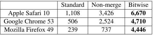
The environment used in this experiment was OS X 10.11.6 with 2.2 GHz Intel Core i7. The code was micro-benchmarked by Benchmark.js 2.1.0, developed by Mathias Bynens2_{, under the following web} browsers: Apple Safari 10.0 (with the JavaScript engine JavaScriptCore, also known as Nitro), Google Chrome 53.0.2785.143 (V8), and Mozilla Firefox 49.0.1 (SpiderMonkey). The experimental results are shown below.

Standard Non-merge Bitwise Apple Safari 10 1,108 3,426 6,670

Google Chrome 53 506 2,524 4,710

Mozilla Firefox 49 239 737 4,446

Table 2: Performance of each feature hashing implementation. Higher is better. Unit: 1k ops/sec.

The results in this table show that the bitwise version is more than five times faster than the standard one in all environments.

As we see, Safari was faster than the other browsers, possibly because the code was run under Apple’s OS. Firefox was slightly slower than Chrome in general settings, but with asm.js enabled it achieved almost the same performance.

In conclusion, the bitwise feature hashing can offer powerful performance improvement when the task involves a number of features and processing those features is the bottleneck of the learning system.

6 Conclusions

This paper showed that pipelining compression methods for machine learning can achieve a succinct model, both theoretically and practically. Although each technique is classical and well-studied, our re-sult is significant in that these techniques actually complement each other, leading to drastic compression without harming the predictive power. We also examined bitwise feature hashing, a subtle but powerful modification for improving processing performance. In future work, we will try to incorporate other compression techniques to build various pipeline configurations and compare the performance of each configuration.

Acknowledgements

This work was supported by CREST, Japan Science and Technology Agency (JST). We are grateful to three anonymous reviewers for their helpful comments.

References

Bernd Bohnet. 2010. Very High Accuracy and Fast Dependency Parsing is not a Contradiction. InProceedings of

the 23rd International Conference on Computational Linguistics (COLING ’10), pages 89–97.

Wenlin Chen, James T. Wilson, Stephen Tyree, Kilian Q. Weinberger, and Yixin Chen. 2015. Compressing Neural

Networks with the Hashing Trick. Proceedings of the 32nd International Conference on Machine Learning,

pages 2285–2294, apr.

Cisco Systems. 2016. The Zettabyte Era: Trends and Analysis. Technical report.

Michael Curtiss, Iain Becker, Tudor Bosman, Sergey Doroshenko, Lucian Grijincu, Tom Jackson, Sandhya Kun-natur, Soren Lassen, Philip Pronin, Sriram Sankar, Guanghao Shen, Gintaras Woss, Chao Yang, and Ning

Zhang. 2013. Unicorn: A System for Searching the Social Graph. Proceedings of the VLDB Endowment,

6(11):1150–1161, aug.

John Duchi and Yoram Singer. 2009. Efficient Online and Batch Learning using Forward Backward Splitting.

Journal of Machine Learning Research, 10:2873–2898.

John Duchi, Elad Hazan, and Yoram Singer. 2011. Adaptive Subgradient Methods for Online Learning and

Stochastic Optimization. Journal of Machine Learning Research, 12:2121–2159.

Peter Elias. 1974. Efficient Storage and Retrieval by Content and Address of Static Files. Journal of the ACM, 21(2):246–260.

Robert M. Fano. 1971. On the Number of Bits Required to Implement An Associative Memory. Technical report, Memorandum 61, Computer Structures Group, MIT, Cambridge, MA.

Kuzman Ganchev and Mark Dredze. 2008. Small Statistical Models by Random Feature Mixing. InProceedings

of the ACL08 HLT Workshop on Mobile Language Processing, pages 19–20.

Daniel Golovin, D. Sculley, H. Brendan McMahan, and Michael Young. 2013. Large-Scale Learning with Less

RAM via Randomization. Proceedings of the 30th International Conference on Machine Learning, 28:325–333,

mar.

Alexander Golynski, Alessio Orlandi, Rajeev Raman, and S. Srinivasa Rao. 2014. Optimal Indexes for Sparse Bit Vectors.Algorithmica, 69(4):906–924, aug.

Roberto Grossi and Jeffrey Scott Vitter. 2005. Compressed Suffix Arrays and Suffix Trees with Applications to

Text Indexing and String Matching. SIAM Journal on Computing, 35(2):378–407, jan.

Masato Hagiwara and Satoshi Sekine. 2014. Lightweight Client-Side Chinese/Japanese Morphological Analyzer

Based on Online Learning. InProceedings of COLING 2014, the 25th International Conference on

Computa-tional Linguistics: System Demonstrations, pages 39–43.

Song Han, Jeff Pool, John Tran, and William J. Dally. 2015. Learning bothWeights and Connections for Efficient

Neural Networks. InAdvances in Neural Information Processing Systems 28, pages 1135–1143.

Song Han, Huizi Mao, and William J. Dally. 2016. Deep Compression: Compressing Deep Neural Networks with

Pruning, Trained Quantization and Huffman Coding. InInternational Conference on Learning Representations.

John Lafferty, Andrew McCallum, and Fernando Pereira. 2001. Conditional Random Fields : Probabilistic Models

for Segmenting and Labeling Sequence Data. InProceedings of the 18th International Conference on Machine

Learning, pages 282–289.

Stuart P. Lloyd. 1982. Least Squares Quantization in PCM.IEEE Transactions on Information Theory, 28(2):129–

137.

Andrew Y. Ng. 2004. Feature selection, L1 vs. L2 regularization, and rotational invariance. InProceedings of the 21 st International Conference on Machine Learning.

Daisuke Okanohara and Kunihiko Sadakane. 2007. Practical Entropy-Compressed Rank / Select Dictionary. In

Proceedings of the 9th Workshop on Algorithm Engineering and Experiments (ALENEX), pages 60–70.

Naoaki Okazaki. 2007. CRFsuite: a fast implementation of conditional random fields (CRFs).

Giuseppe Ottaviano and Rossano Venturini. 2014. Partitioned Elias-Fano Indexes. InProceedings of the 37th

Fei Sha and Fernando Pereira. 2003. Shallow parsing with conditional random fields. In Proceedings of the 2003 Conference of the North American Chapter of the Association for Computational Linguistics on Human

Language Technology, number June, pages 134–141, Morristown, NJ, USA. Association for Computational

Linguistics.

Ehsan Shareghi, Matthias Petri, Gholamreza Haffari, and Trevor Cohn. 2015. Compact, Efficient and Unlimited

Capacity: Language Modeling with Compressed Suffix Trees. In Proceedings of the 2015 Conference on

Empirical Methods in Natural Language Processing, pages 2409–2418.

Qinfeng Shi, James Petterson, Gideon Dror, John Langford, Alex Smola, and S.V.N. Vishwanathan. 2009. Hash

Kernels for Structured Data. Journal of Machine Learning Research, 10:2615–2637.

Jeffrey Sorensen and Cyril Allauzen. 2011. Unary Data Structures for Language Models. InINTERSPEECH

2011, pages 1425–1428.

Erik F. Tjong Kim Sang and Sabine Buchholz. 2000. Introduction to the CoNLL-2000 Shared Task: Chunking.

InProceedings of CoNLL-2000 and LLL-2000.

Yoshimasa Tsuruoka, Jun’ichi Tsujii, and Sophia Ananiadou. 2009. Stochastic Gradient Descent Training for

L1-regularized Log-linear Models with Cumulative Penalty. InProceedings of the 47th Annual Meeting of the

ACL and the 4th IJCNLP of the AFNLP, pages 477–485.

Sebastiano Vigna. 2013. Quasi-Succinct Indices. InProceedings of the Sixth ACM International Conference on

Web Search and Data Mining - WSDM ’13, pages 83–92, New York, New York, USA. ACM Press.

Taro Watanabe, Hajime Tsukada, and Hideki Isozaki. 2009. A Succinct N-gram Language Model. InProceedings

of the ACL-IJCNLP 2009 Conference Short Papers, pages 341–344.