Sentiment Classification with Graph Co Regularization

Sentiment Classification with Graph Co-Regularization

Guangyou Zhou, Jun Zhao, and Daojian Zeng

National Laboratory of Pattern Recognition Institute of Automation, Chinese Academy of Sciences

95 Zhongguancun East Road, Beijing 100190, China {gyzhou,jzhao,djzeng}@nlpr.ia.ac.cn

Abstract

Sentiment classification aims to automatically predict sentiment polarity (e.g., positive or neg-ative) of user-generated sentiment data (e.g., reviews, blogs). To obtain sentiment classifica-tion with high accuracy, supervised techniques require a large amount of manually labeled data. The labeling work can be time-consuming and expensive, which makes unsupervised (or semi-supervised) sentiment analysis essential for this application. In this paper, we propose a novel algorithm, called graph co-regularized non-negative matrix tri-factorization (GNMTF), from the geometric perspective. GNMTF assumes that if two words (or documents) are sufficiently close to each other, they tend to share the same sentiment polarity. To achieve this, we encode the geometric information by constructing the nearest neighbor graphs, in conjunction with a non-negative matrix tri-factorization framework. We derive an efficient algorithm for learning the factorization, analyze its complexity, and provide proof of convergence. Our empirical study on two open data sets validates that GNMTF can consistently improve the sentiment classification accuracy in comparison to the state-of-the-art methods.

1 Introduction

Recently, sentiment classification has gained a wide interest in natural language processing (NLP) com-munity. Methods for automatically classifying sentiments expressed in products and movie reviews can roughly be divided into supervised and unsupervised (or semi-supervised) sentiment analysis. Super-vised techniques have been proved promising and widely used in sentiment classification (Pang et al., 2002; Pang and Lee, 2008; Liu, 2012). However, the performance of these methods relies on manually labeled training data. In some cases, the labeling work may be time-consuming and expensive. This motivates the problem of learning robust sentiment classification via unsupervised (or semi-supervised) paradigm.

A traditional way to perform unsupervised sentiment analysis is the lexicon-based method (Turney, 2002; Taboada et al., 2011). Lexicon-based methods employ a sentiment lexicon to determine overall sentiment orientation of a document. However, it is difficult to define a universally optimal sentiment lexicon to cover all words from different domains (Lu et al., 2011a). Besides, most semi-automated lexicon-based methods yield unsatisfactory lexicons, with either high coverage and low precision or vice versa (Ng et al., 2006). Thus it is challenging for lexicon-based methods to accurately identify the overall sentiment polarity of users generated sentiment data. Recently, Li et al. (2009) proposed a constrained non-negative matrix tri-factorization (CNMTF) approach to sentiment classification, with a domain-independent sentiment lexicon as prior knowledge. Experimental results show that CNMTF achieves state-of-the-art performance.

From the geometric perspective, the data points (words or documents) may be sampled from a distribu-tion supported by a low-dimensional manifold embedded in a high-dimensional space (Cai et al., 2011). This geometric structure, meaning that two words (or documents) sufficiently close to each other tend to share the same sentiment polarity, should be preserved during the matrix factorization. Research studies This work is licensed under a Creative Commons Attribution 4.0 International Licence. Page numbers and proceedings footer are added by the organisers. Licence details: http:// creativecommons.org/licenses/by/4.0/

have shown that learning performance can be significantly enhanced in many real applications (e.g., text mining, computer vision, etc.) if the geometric structure is exploited (Roweis and Saul, 2000; Tenen-baum et al., 2000). However, CNMTF fails to exploit the geometric structure, it is not clear whether this geometric information is useful for sentiment classification, which remains an under-explored area. This paper is thus designed to fill the gap.

In this paper, we propose a novel algorithm, called graph co-regularized non-negative matrix tri-factorization (GNMTF). We construct two affinity graphs to encode the geometric information under-lying the word space and the document space, respectively. Intuitively, if two words or documents are sufficiently close to each other, they tend to share the same sentiment polarity. Taking these two graphs as co-regularization for the non-negative matrix tri-factorization, leading to the better sentiment polarity prediction which respects to the geometric structures of the word space and document space. We also de-rive an efficient algorithm for learning the tri-factorization, analyze its complexity, and provide proof of convergence. Empirical study on two open data sets shows encouraging results of the proposed method in comparison to state-of-the-art methods.

The remainder of this paper is organized as follows. Section 2 introduces the basic concept of matrix tri-factorization. Section 3 describes our graph co-regularized non-negative matrix tri-factorization (GN-MTF) for sentiment classification. Section 4 presents the experimental results. Section 5 introduces the related work. In section 6, we conclude the paper and discuss future research directions.

2 Preliminaries

2.1 Non-negative Matrix Tri-factorization

Li et al. (2009) proposed a matrix factorization based framework for unsupervised (or semi-supervised) sentiment analysis. The proposed framework is built on the orthogonal non-negative matrix tri-factorization (NMTF) (Ding et al., 2006). In these models, a term-document matrixX= [x1,· · · ,xn]∈ Rm×n_{is approximated by three factor matrices that specify cluster labels for words and documents by}

solving the following optimization problem:

min

U,H,V≥0O=X−UHV

T2

F+σ1UTU−I

2

F+σ2VTV−I

2

F (1)

whereσ1 andσ2 are the shrinkage regularization parameters,U = [u1,· · · ,uk] ∈Rm+×k is the word-sentiment matrix,V = [v1,· · · ,vn]∈Rn+×k is the document-sentiment matrix, andkis the number of sentiment classes for documents. Our task is polarity sentiment classification (positive or negative), i.e.,

k= 2. For example,Vi1 = 1(orUi1 = 1) represents that the sentiment polarity of documenti(or word

i) is positive, andVi2 = 1(orUi2 = 1) represents that the sentiment polarity of documenti(or wordi) is negative.Vi∗ = 0(orUi∗= 0) represents unknown, i.e., the documenti(or wordi) is neither positive or negative. H∈Rk₊×k provides a condensed view ofX;∥ · ∥F is the Frobenius norm andIis ak×k

identity matrix with all entries equal to 1. Based on the shrinkage methodology, we can approximately satisfy the orthogonality constraints forUandVby preventing the second and third terms from getting too large.

2.2 Constrained NMTF

Lexical knowledge in the form of the polarity of words in the lexicon can be introduced in matrix tri-factorization. By partially specifying word polarity viaU, the lexicon influences the sentiment prediction

Vover documents. Following the literature (Li et al., 2009), letU0 represent lexical prior knowledge about sentiment words in the lexicon, e.g., if word i is positive (U0)i1 = 1 while if it is negative

(U0)i2 = 1, and if it does not exist in the lexicon(U0)i∗ = 0. Li et al. (2009) also investigated that we had a few documents manually labeled for the purpose of capturing some domain-specific connotations. LetV0denote the manually labeled documents, if the document expresses positive sentiment(V0)ii= 1,

and(V0)i2 = 1for negative sentiment. Therefore, the semi-supervised learning with lexical knowledge can be written as:

min

U,H,V≥0O+αTr

[

where Tr(·) denotes the trace of a matrix, α > 0 and β > 0 are the parameters which control the contribution of lexical prior knowledge and manually labeled documents.Cu_{∈ {0,1}}m×m_{is a diagonal}

matrix whose entryCu

ii = 1 if the category of the i-th word is known and Cuii = 0 otherwise. Cv ∈ {0,1}n×n_{is a diagonal matrix whose entryC}v

ii = 1if the category of thei-th document is labeled and Cv

ii= 0otherwise.

3 Graph Co-regularized Non-negative Matrix Tri-factorization

In this section, we introduce our proposed graph co-regularized non-negative matrix tri-factorization (GNMTF) algorithm which avoids this limitation by incorporating the geometrically based co-regularization.

3.1 Model Formulation

Based on the manifold assumption (Belkin and Niyogi, 2001), if two documentsxiandxjare sufficiently

close to each other in the intrinsic geometric of the documents distribution, then their sentiment polarity

viandvjshould be close. In order to model the geometric structure, we construct a document-document

graphGv_{. In the graph, nodes represent documents in the corpus and edges represent the affinity between}

the documents. The affinity matrixWv _∈Rn×n_{of the graphG}v_{is defined as}

Wijv = {

cos(xi,xj) ifxi∈ Np(xj)orxj∈ Np(xi)

0 otherwise (3)

whereNp(xi)represents thep-nearest neighbors of documentxi. Many matrices, e.g., 0-1 weighting,

textual similarity and heat kernel weighting (Belkin and Niyogi, 2001), can be used to obtain nearest neighbors of a document, and further define the affinity matrix. Since Wv

ij in our paper is only for

measuring the closeness, we only use the simple textual similarity and do not treat the different weighting schemes separately due to the limited space. For further information, please refer to (Cai et al., 2011).

Preserving the geometric structure in the document space is reduced to minimizing the following loss function:

Rv_{= 1}

2

n ∑

i,j=1

vi−vj2₂Wvij= n ∑

i=1

vT iviDvii−

n ∑

i,j=1

vT ivjWijv

=Tr(VTDvV)−Tr(VTWvV) =Tr(VTLvV)

(4)

whereDv _∈Rn×n_{is a diagonal matrix whose entries are column (or row, sinceD}v _{is symmetric) sums}

ofWv_,Dv

ii=∑nj=1Wvij, andLv =Dv−Wvis the Laplacian matrix (Chung, 1997) of the constructed

graphGv_.

Similarly to document-document geometric structure, if two words wi = [xi1,· · · ,xin]andwj =

[xj1,· · ·,xjn]are sufficiently close to each other in the intrinsic geometric of the words distribution,

then their sentiment polarityuianduj should be close. In order to model the geometric structure in the

word space, we construct a word-word graphGu_{. In the graph, nodes represent distinct words and edges}

represent the affinity between words. The affinity matrixWu_∈Rm×m_{of the graphG}u_{is defined as}

Wu ij=

{

cos(wi,wj) ifwi∈ Np(wj)orwj∈ Np(wi)

0 otherwise (5)

whereNp(wj)represents thep-nearest neighbor of wordwj. Here, we represent a termwj as a

docu-ment vector[xj1,· · ·,xjn]. To measure the closeness of two words, a common way is to calculate the similarity of their vector representations. Although there are several ways (e.g., co-occurrence infor-mation, semantic similarity computed by WordNet, Wikipedia, or search engine have been empirically studied in NLP literature (Hu et al., 2009)) to define the affinity matrixWu_{, we do not treat the different}

ways separately and leave this investigation for future work.

Preserving the geometric structure in the word space is reduced to minimizing the following loss function:

Ru_{= 1}

2

m ∑

i,j=1

_ui−uj2

2W

u

whereLu _{= D}u _−Wu _{is the Laplacian matrix of the constructed graphG}u_{, andD}u _{∈ R}m×m _{is a}

diagonal matrix whose entries areDu

ii=∑mj=1Wuij.

Finally, we treat unsupervised (or semi-supervised) sentiment classification as a clustering problem, employing lexical prior knowledge and partial manually labeled data to guide the learning process. More-over, we introduce the geometric structures from both document and word sides as co-regularization. Therefore, our proposed unsupervised (or semi-supervised) sentiment classification framework can be mathematically formulated as solving the following optimization problem:

min

U,H,V≥0L=X−UHV

T2

F+σ1UTU−I

2

F+σ2VTV−I

2

F

+αTr[(U−U0)TCu(U−U0)]+γTr(UTLuU)

+βTr[(V−V0)TCv(V−V0)]+δTr(VTLvV)

(7)

whereδ > 0andγ > 0are parameters which control the contributions of document space and word space geometric information, respectively. With the optimization results, the sentiment polarity of a new documentxican be easily inferred byf(xi) = arg maxj∈{p, n}Vij.

3.2 Learning Algorithm

We present the solution to the GNMTF optimization problem in equation (7) as the following theorem. The theoretical aspects of the optimization are presented in the next subsection.

Theorem 3.1. UpdatingU,HandVusing equations (8)∼(10) will monotonically decrease the objec-tive function in equation (7) until convergence.

U←U◦

[

XVHT_+σ

1U+αCuU0+γWuU ] [

UHVT_VHT_+σ1UUT_U+αCu_U+γDu_U] (8)

H←H◦

[

UT_XV] [

UT_UHVT_V] (9)

V←V◦

[

XT_UH+σ

2V+βCvV0+δWvV ] [

VHT_UT_UH+σ2VVT_V+βCv_V+δDv_V] (10)

where operator◦is element-wise product and [_[·_·]_] is element-wise division.

Based on Theorem 3.1, we note that the multiplicative update rules given by equations (8)∼(10) are obtained by extending the updates of standard NMTF (Ding et al., 2006). A number of techniques can be used here to optimize the objective function in equation (7), such as alternating least squares (Kim and Park, 2008), the active set method (Kim and Park, 2008), and the projected gradients approach (Lin, 2007). Nonetheless, the multiplicative updates derived in this paper has reasonably fast convergence behavior as shown empirically in the experiments.

3.3 Theoretical Analysis

In this subsection, we give the theoretical analysis of the optimization, convergence and computational complexity. Without loss of generality, we only show the optimization ofUand formulate the Lagrange function with constraints as follows:

L(U) =X−UHVT2

F+σ1UTU−I

2

F+αTr [

(U−U0)TCu(U−U0)]+Tr(ΨUT) (11)

whereΨis the Lagrange multiplier for the nonnegative constraintU ≥0. The partial derivative ofL(U)w.r.t.Uis

▽UL(U) =−2XVHT+ 2UHVTVHT+ 2σ1UUTU−2σ1U

+ 2αCu_U−2αCu_U

Using the Karush-Kuhn-Tucker (KKT) (Boyd and Vandenberghe, 2004) conditionΨ◦U=0, we can obtain

▽UL(U)◦U=[UHVTVHT+σ1UUTU+αCuU+γDuU]◦U −[XVHT_+σ

1U+αCuU0+γWuU]◦U=0

This leads to the update rule in equation (8). Following the similar derivations as shown above, we can obtain the updating rules for all the other variablesHandVin GNMTF optimization, as shown in equations (9) and (10).

3.3.1 Convergence Analysis

In this subsection, we prove the convergence of multiplicative updates given by equations (8)∼(10). We first introduce the definition of auxiliary function as follows.

Definition 3.1. F(Y,Y′_{)is an auxiliary function forL(Y)ifL(Y)≤ F(Y,Y}′_{)and equality holds if}

and only ifL(Y) =F(Y,Y).

Lemma 3.1. (Lee and Seung, 2001) IfF is an auxiliary function forL,Lis non-increasing under the updateY(t+1)_{= arg minYF(Y,Y}(t)₎

Proof. By Definition 3.1,L(Y(t+1)_{)≤ F(Y}(t+1)_,Y(t)_{)≤ F(Y}(t)_,Y(t)_{) =L(Y}(t)₎

Theorem 3.2. Let function

F(Uij,U(ijt)) =L(U(ijt)) +L

′

(U(ijt))(Uij−U(ijt))

+

[

UHVT_VHT_+σ

1UUTU+αCuU+γDuU]_ij

Uij

(

Uij−U(ijt)

) (12)

be a proper auxiliary function forL(Uij), whereL′(Uij) = [▽UL(U)]ij is the first-order derivatives ofL(Uij)with respect toUij.

Theorem 3.2 can be proved similarly to (Ding et al., 2006). Due to limited space, we omit the details of the validation. Based on Lemmas 3.1 and Theorem 3.2, the update rule for U can be obtained by minimizingF(U(_ijt+1),U_ij(t)). When setting▽_U(t+1)

ij F(U

(t+1)

ij ,U(ijt)), we can obtain

U(_ijt+1)=U(_ijt)

[

XVHT_+σ

1U+αCuU0+γWuU]_ij

[

UHVT_VHT_+σ1UUT_U+αCu_U+γDu_U] ij

By Lemma 3.1 and Theorem 3.2, we have L(U(0)_{) = F(U}(0)_,U(0)_{) ≥ F(U}(1)_,U(0)_{) ≥}

F(U(1)_,U(1)_{) = L(U}(1)_{) ≥ · · · ≥ L(U}(Iter)_{), whereIter denotes the number of iteration number.} Therefore,U is monotonically decreasing. Since the objective functionL is lower bounded by 0, the correctness and convergence of Theorem 3.1 is validated.

3.3.2 Time Complexity Analysis

In this subsection, we discuss the time computational complexity of the proposed algorithm GNMTF. Besides expressing the complexity of the algorithm using bigOnotation, we also count the number of arithmetic operations to provide more details about running time. We show the results in Table 1, where

m≫kandn≫k.

Based on the updating rules summarized in Theorem 3.1, it it not hard to count the arithmetic operators of each iteration in GNMTF. It is important to note thatCu_{is a diagonal matrix, the nonzero elements on}

each row ofCu_{is 1. Thus, we only need zero addition andmkmultiplications to computeC}u_U.

Simi-larly, forCu_U

0,CvV,CvV0,DuUandDvV, we also only need zero addition andmkmultiplications for each of them. Besides, we also note thatWu_{is a sparse matrix, if we use ap-nearest neighbor graph,}

the average nonzero elements on each row ofWu _{isp. Thus, we only needmpk additions and mpk}

multiplications to computeWu_{U. Similarly, forW}v_{V, we need the same operation counts asW}u_U.

addition multiplication division overall GNMTF:U 2k3_{+ (2m+n)k}2_{+m(n+p)k 2k}3_{+ (2m+n)k}2_{+m(n+p+ 7)k mk O(mnk)}

GNMTF:H 2k3_{+ (m+n+ 2)k}2_{+mnk 2k}3_{+ (m+n+ 1)k}2_{+mnk k}2 _O(mnk)

GNMTF:V 2k3_{+ (2n+m)k}2_{+n(m+p)k 2k}3_{+ (2n+m)k}2_{+n(m+p+ 7)k nk O(mnk)} Table 1: Computational operation counts for each iteration in GNMTF.

4 Experiments

4.1 Data Sets

Sentiment classification has been extensively studied in the literature. Among these, a large majority proposed experiments performed on the benchmarks made of Movies Reviews (Pang et al., 2002) and Amazon products (Blitzer et al., 2007).

Movies data This data set has been widely used for sentiment analysis in the literature (Pang et al., 2002), which consists of 1000 positive and 1000 negative reviews drawn from the IMDB archive of rec.arts.movies.reviews.newsgroups.

Amazon data This data set is heterogeneous, heavily unbalanced and large-scale, a smaller ver-sion has been released. The reduced data set contains 4 product types: Kitchen, Books, DVDs, and Electronics (Blitzer et al., 2007). There are 4000 positive and 4000 negative reviews.1

For these two data sets, we select 8000 words with highest document-frequency to generate the vo-cabulary. Stopwords2_{are removed and a normalized term-frequency representation is used. In order to}

construct the lexical prior knowledge matrixU0, we use the sentiment lexicon generated by (Hu and Liu, 2004). It contains 2,006 positive words (e.g., “beautiful”) and 4,783 negative words (e.g., “upset”).

4.2 Unsupervised Sentiment Classification

Our first experiment is to explore the benefits of incorporating the geometric information in the unsu-pervised paradigm (that isCv _{=0). Therefore, the third part in equation (7) will be ignored. For this}

unsupervised paradigm of GNMTF, we empirically setα=δ =γ = 1,σ1 =σ2 = 1,Iter = 100and run GNMTF 10 repeated times to remove any randomness caused by the random initialization. Due to limited space, we do not present the impacts of the parameters on the learning model. Now we compare our proposed GNMTF with the following four categories of methods:

(1) Lexicon-Based Methods (LBM in short): Taboada et al. (2011) proposed to incorporate intensifi-cation and negation to refine the sentiment score for each document. This is the state-of-the-art lexicon-based method for unsupervised sentiment classification.

(2) Document Clustering Methods: We choose the most representative cluster methods, K-means, NMTF, Information-Theoretic Co-clustering (ITCC) (Dhillon et al., 2003), and Euclidean Co-clustering method (ECC) (Cho et al., 2004). We set the number of clusters as two in these methods. Note that all these methods do not make use of the sentiment lexicon.

(3) Constrained NMTF (CNMTF in short): Li et al. (2009) incorporated the sentiment lexicon into NMTF as a domain-independent prior constraint.

(4) Graph co-regularized Non-negative Matrix Tri-factorization (GNMTF in short): It is a new algo-rithm proposed in this paper. We use cosine similarity for constructing thep-nearest neighbor graph for its simplicity. The number of nearest neighbor pis set to 10 empirically both on document and word spaces.

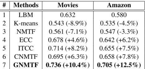
4.2.1 Sentiment Classification Results

The experimental results are reported in Table 2. We perform a significant test, i.e., at-test with a default significant level of 0.05. From Table 2, we can see that (1) Both CNMTF and GNMTF consider the lexical prior knowledge from off-the-shelf sentiment lexicon and achieve better performance than NMTF. This suggests the importance of the lexical prior knowledge in learning the sentiment classification (row

# Methods Movies Amazon

1 LBM 0.632 0.580

2 K-means 0.543 (-8.9%) 0.535 (-4.5%) 3 NMTF 0.561 (-7.1%) 0.547 (-3.3%) 4 ECC 0.678 (+4.6%) 0.642 (+6.2%) 5 ITCC 0.714 (+8.2%) 0.655 (+7.5%) 6 CNMTF 0.695 (+6.3%) 0.658 (+7.8%) 7 GNMTF 0.736 (+10.4%) 0.705 (+12.5%)

Table 2: Sentiment classification accuracy of unsupervised paradigm on the data sets. Improvements of K-means, NMTF, ITCC, ECC, CNMTF and GNMTF over baseline LBM are shown in parentheses.

0 20 40 60 80 100

0.2 0.25 0.3 0.35 0.4 0.45 0.5

(a) Movies data

O

b

je

c

ti

v

e

f

u

n

c

ti

o

n

v

a

lu

e

0 20 40 60 80 100

0.46 0.48 0.5 0.52 0.54 0.56 0.58 0.6 0.62 0.64 0.66

(b) Amazon data

O

b

je

c

ti

v

e

f

u

n

c

ti

o

n

v

a

lu

e

Figure 1: Convergence curves of GNMTF on both data sets.

3 vs. row 6 and row 7); (2) Regardless of the data sets, our GNMTF significantly outperforms state-of-the-art CNMTF and achieves the best performance. This shows the superiority of geometric information and graph co-regularization framework (row 4 vs. row 5, the improvements are statistically significant at

p <0.05).

4.2.2 Convergence Behavior

In subsection 3.3.1, we have shown that the multiplicative updates given by equations (8)∼(10) are convergent. Here, we empirically show the convergence behavior of GNMTF.

Figure 1 shows the convergence curves of GNMTF on Movies and Amazon data sets. From the figure, y-axis is the value of objective function and x-axis denotes the iteration number. We can see that the multiplicative updates for GNMTF converge very fast, usually within 50 iterations.

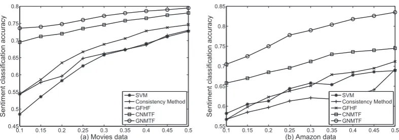
4.3 Semi-supervised Sentiment Classification

In this subsection, we describe our proposed GNMTF with a few labeled documents. For this semi-supervised paradigm of GNMTF, we empirically setIter= 100,σ1 =σ2= 2,α=β =δ=γ = 1and

p= 10on document and word spaces and also run 10 repeated times to remove any randomness caused by the random initialization. Due to limited space, we do not give an in-depth parameter analysis. For CNMTF, we setα = β = 1for fair comparison. We also compare our proposed GNMTF with some representative semi-supervised approaches described in (Li et al., 2009): (1) Semi-supervised learning with local and global consistency (Consistency Method in short) (Zhou et al., 2004); (2) Semi-supervised learning using gaussian fields and harmonic functions (GFHF in short) (Zhu et al., 2003). Besides, we also compare the results of our proposed GNMTF with the representative supervised classification method: support vector machine (SVM), which has been widely used in sentiment classification (Pang et al., 2002).

0.1 0.15 0.2 0.25 0.3 0.35 0.4 0.45 0.5 0.45 0.5 0.55 0.6 0.65 0.7 0.75 0.8

(a) Movies data

S e n ti m e n t c la s s if ic a ti o n a c c u ra c y SVM Consistency Method GFHF CNMTF GNMTF

0.1 0.15 0.2 0.25 0.3 0.35 0.4 0.45 0.5 0.55 0.6 0.65 0.7 0.75 0.8 0.85

(b) Amazon data

S e n ti m e n t c la s s if ic a ti o n a c c u ra c y SVM Consistency Method GFHF CNMTF GNMTF

Figure 2: Sentiment classification accuracy vs. different percentage of labeled documents, where x-axis denotes the number of documents labeled as a fraction of the original labeled documents.

5 Related Work

Sentiment classification has gained widely interest in NLP community, we point the readers to recent books (Pang and Lee, 2008; Liu, 2012) for an in-depth survey of literature on sentiment analysis.

Methods for automatically classifying sentiments expressed in products and movie reviews can roughly be divided into supervised and unsupervised (or semi-supervised) sentiment analysis. Super-vised techniques have been proved promising and widely used in sentiment classification (Pang et al., 2002; Pang and Lee, 2008; Liu, 2012). However, the performance of these methods relies on manually labeled training data. In some cases, the labeling work may be time-consuming and expensive. This motivates the problem of learning robust sentiment classification via unsupervised (or semi-supervised) paradigm.

The most representative way to perform semi-supervised paradigm is to employ partial labeled data to guide the sentiment classification (Goldberg and Zhu, 2006; Sindhwani and Melville, 2008; Wan, 2009; Li et al., 2011). However, we do not have any labeled data at hand in many situations, which makes the unsupervised paradigm possible. The most representative way to perform unsupervised paradigm is to use a sentiment lexicon to guide the sentiment classification (Turney, 2002; Taboada et al., 2011) or learn sentiment orientation via a matrix factorization clustering framework (Li et al., 2009; ?; Hu et al., 2013). In contrast, we perform sentiment classification with the different model formulation and learning algorithm, which considers both word-level and document-level sentiment-related contextual information (e.g., the neighboring words or documents tend to share the same sentiment polarity) into a unified framework. The proposed framework makes use of the valuable geometric information to compensate the problem of lack of labeled data for sentiment classification. In addition, some researchers also explored the matrix factorization techniques for other NLP tasks, such as relation extraction (Peng and Park, 2013) and question answering (Zhou et al., 2013)

Besides, many studies address some other aspects of sentiment analysis, such as cross-domain senti-ment classification (Blitzer et al., 2007; Pan et al., 2010; Hu et al., 2011; Bollegala et al., 2011; Glorot et al., 2011), cross-lingual sentiment classification (Wan, 2009; Lu et al., 2011b; Meng et al., 2012) and imbalanced sentiment classification (Li et al., 2011), which are out of scope of this paper.

6 Conclusion and Future Work

There are some ways in which this research could be continued. First, some other ways should be considered to construct the graphs (e.g., hyperlinks between documents, synonyms or co-occurrences between words). Second, we will try to extend the proposed framework for other aspects of sentiment analysis, such as cross-domain or cross-lingual settings.

Acknowledgments

This work was supported by the National Natural Science Foundation of China (No. 61303180 and No. 61272332), the Beijing Natural Science Foundation (No. 4144087), CCF Opening Project of Chi-nese Information Processing, and also Sponsored by CCF-Tencent Open Research Fund. We thank the anonymous reviewers for their insightful comments.

References

M. Belkin and P. Niyogi. 2001. Laplacian eigenmaps and spectral techniques for embedding and clustering. In

Proceedings of NIPS, pages 585-591.

J. Blitzer, M. Dredze and F. Pereira. 2007. Biographies, bollywood, boom-boxes and blenders: domain adaptation for sentiment classification. InProceedings of ACL, pages 440-447.

D. Bollegala, D. Weir, and J. Carroll. 2011. Using multiples sources to construct a sentiment sensitive thesaurus.

InProceedings of ACL, pages 132-141.

S. Boyd and L. Vandenberghe. 2004.Convex Optimization. Cambridge university press.

D. Cai, X. He, J. Han, and T. Huang. 2011. Graph regularized non-negative matrix factorization for data represen-tation. IEEE Transactions on Pattern Analysis and Machine Intelligence, 33(8): 1548-1560.

H. Cho, I. Dhillon, Y. Guan, and S. Sra. 2004. Minimum sum squared residue co-clutering of gene expression data. InProceedings of SDM, pages 22-24.

F. Chung. 1997. Spectral graph theory.Regional Conference Series in Mathematics, Volume 92.

I. Dhillon, S. Mallela, and D. Modha. 2003. Information-theoretic Co-clustering. InProceedings of KDD, pages

89-98.

C. Ding, T. Li, W. Peng, and H. Park. 2006. Orthogonal non-negative matrix tri-factorization for clustering. In

Proceedings of KDD, pages 126-135.

X. Glorot, A. Bordes, and Y. Bengio. 2011. Domain adaptation for larage-scale sentiment classification: a deep learning approach. InProceedings of ICML.

A. Goldberg and X. Zhu. 2006. Seeing stars when there aren’t many stars: graph-based semi-supervised learning

for sentiment categorization. InProceedings of NAACL Workshop.

Y. He, C. Lin and H. Alani. 2011. Automatically extracting polarity-bearing topics for cross-domain sentiment classification. InProceedings of ACL, pages 123-131.

M. Hu and B. Liu. 2004. Mining and summarizing customer reviews. InProceedings of KDD.

X. Hu, J. Tang, H. Gao, and H. Liu. 2013. Unsupervised sentiment analysis with emotional signals. InProceedings

of WSDM.

X. Hu, N. Sun, C. Zhang, and T. Chua. 2009. Exploiting internal and external semantics for the clustering of short

texts using world knowldge. InProceedings of CIKM, pages 919-928.

H. Kim and H. Park. 2008. Non-negative matrix factorization based on alternating non-negativity constrained least squares and active set method.SIAM J Matrix Anal Appl, 30(2):713-730.

D. Lee and H. Seung. 2001. Algorithms for non-negative matrix factorization. InProceedings of NIPS.

S. Li, Z. Wang, G. Zhou, and S. Lee. 2011. Semi-supervised learning for imbalanced sentiment classification. In

T. Li, Y. Zhang, and V. Singhwani. 2009. A non-negative matrix tri-factorization approach to sentiment classifica-tion with lexical prior knowledge. InProceedings of ACL, pages 244-252.

C. Lin. 2007. Projected gradient methods for nonnegative matrix factorization. Neural Comput,

19(10):2756-2779.

B. Liu. 2012. Sentiment analysis and opinion mining. Morgan & Claypool Publishers.

B. Lu, C. Tan, C. Cardie, and B. Tsou. 2011. Joint bilingual sentiment classification with unlabeled parallel corpora. InProceedings of ACL, pages 320-330.

Y. Lu, M. Castellanos, U. Dayal, and C. Zhai. 2011. Automatic construction of a context-aware sentiment lexicon:

an optimization approach. InProceedings of WWW, pages 347-356.

X. Meng, F. Wei, X. Liu, M. Zhou, G. Xu, and H. Wang. 2012. Cross-lingual mixture model for sentiment classification. InProceedings of ACL, pages 572-581.

V. Ng, S. Dasgupta, and S. Arifin. 2006. Examing the role of linguistic knowlege sources in the automatic identification and classificaton of reviews. InProceedings of ACL.

S. Pan, X. Ni, J. Sun, Q. Yang, and Z. Chen. 2010. Cross-domain sentiment classification via spectral feature

alignment. InProceedings of WWW.

B. Pang and L. Lee. 2008. Opinion mining and sentiment analysis. Foundations and Trends in Informaiton

Retrieval, pages 1-135.

B. Pang, L. Lee, S. Vaithyanathan. 2002. Thumbs up? sentiment classification using machine learning techniques.

InProceedings of EMNLP, pages 79-86.

S. Riedel, L. Yao, A. McCallum, and B. Marlin. 2013. Relation extraction with matrix factorization and universal

schemas. InProceedings of NAACL.

W. Peng and D. Park. 2011. Generative adjective sentiment dictionary for social media sentiment analysis using constrained nonnegative matrix factorization. InProceedings of ICWSM.

S. Roweis and L. Saul. 2000. Nonlinear dimensionality reduction by locally linear embedding. Science,

290(5500):2323-2326.

V. Sindhwani and P. Melville. 2008. Document-word co-regulariztion for semi-supervised sentiment analysis. In

Proceedings of ICDM, pages 1025-1030.

J. Tenenbaum, V. Silva, and J. Langford. 2000. A global geometric framework for nonlinear dimensionality reduction. Science, 290(5500):2319-2323.

M. Taboada, J. Brooke, M. Tofiloski, K. Voll, and M. Stede. 2011. Lexicon-based methods for sentiment analysis.

Computational Linguistics.

P. Turney. 2002. Thumbs up or thumbs down?: semantic orientation applied to unsupervised classification of reviews. InProceedings of ACL, pages 417-424.

X. Wan. 2009. Co-training for cross-lingual sentiment classification. InProceedings of ACL, pages 235-243. D. Zhou, Q. Bousquet, T. Lal, J. Weston, and B. Scholkopf. 2004. Learning with local and global consistency. In

Proceedings of NIPS.

G. Zhou, F. Liu, Y. Liu, S. He, and J. Zhao. 2013. Statistical machine translation improves question retrieval in

community question answering via matrix factorization. InProceedings of ACL, pages 852-861.