Variational methods in surface parameterization

(1)

Variational Methods in Surface Parameterization

Thesis by Nathan J. Litke

In Partial Fulfillment of the Requirements for the Degree of

Doctor of Philosophy

California Institute of Technology Pasadena, California

2005

(2)

c

2005

(3)

(4)

Acknowledgements

There are many people whose guidance and support made this work possible. First and foremost, I thank my advisor, Peter Schr¨oder, for his wisdom and generosity. Through his kind guidance I have learned invaluable skills which have shaped me as a researcher and as a scientist. For these experiences I am forever grateful.

I am also deeply indebted to my thesis committee whose encouragement and enthusiasm not only elevated this work but have also profoundly affected me personally and philosophically. Alan Barr has been a voice of sage counsel, whose timely advice has gently steered me along an enlight-ened path. Mathieu Desbrun has graciously shared his brilliant intellect to help me overcome even my most trivial conundrums, and his kindness and optimism have been felt far beyond my academic pursuits. Martin Rumpf has been my colleague, my mentor and my friend through many exciting discoveries, and his kind hospitality during my time in Germany made these months the highlight of my graduate career.

I have been extremely fortunate to work with many exceptionally talented and gifted researchers over the years. Adi Levin, Andrei Khodakovsky, Ulrich Clarenz and Marc Droske have been a pleasure to work with and have enriched my experiences both in research and personally. My peers in the Multires Modeling Group and abroad made the journey fulfilling and entertaining, and the support that I received from my friends has truly provided me with the experience of a lifetime. Eitan Grinspun, Liliya Kharevych, Catherine Mastromarino, Gerhard Bendels, Mark Meyer, Tran Gieng, Zo¨e Wood, Sharif Elcott, Ilja Friedel, Steven Schkolne and Boris Springborn have left me with countless unforgettable memories.

(5)

Abstract

A surface parameterization is a function that maps coordinates in a 2-dimensional parameter space to points on a surface. This thesis investigates two kinds of parameterizations for surfaces that are disc-like in shape. The first is a map from a region of the plane to the surface. The second is a mapping from one surface to another, which defines a correspondence between them. The main challenge in both cases is the construction of a smooth map with low distortion. In this thesis we present a variational approach to surface parameterization that addresses these challenges.

The first contribution of this thesis is the development of a variational framework for parame-terizations. This framework encompasses the mapping of a region of the plane to a surface that is isomorphic to a disc, and the mapping between such surfaces. It is based on the rich mathematical theory built up over decades in the study of rational mechanics. Because of its roots in mechanics, our parameterizations are guaranteed to be smooth and locally bijective, and optimal parameteriza-tions which minimize a variational energy are known to exist. A proof of existence is given for the case of optimal parameterizations in the plane.

Our second contribution is a set of algorithms to construct parameterizations for surface trian-gulations. We describe in detail free-boundary methods that use standard numerical optimization algorithms for the computation of optimal parameterizations. A flexible set of parameters is offered to the user to formulate preferences for the trade-off between angle, area and length distortion in parameterizations in the plane. In the specification of a correspondence between surfaces, we pro-vide user control through feature lines which are mapped as sets onto corresponding feature lines. Additionally we allow for a partial correspondence of the surfaces which is particularly important for correlating surfaces with boundaries.

(6)

presence of large deformations in the parameterizations and the stability of our parameterizations is demonstrated under different discretizations of the surfaces.

(7)

List of Figures

2.1 The optimal parameterization functionx[φ] . . . 11

2.2 A physical interpretation of the matching deformation . . . 18

2.3 The matching functionφM . . . 19

3.1 Overview of the surface parameterization algorithm . . . 26

3.2 The parameterization optimization algorithm . . . 29

3.3 The step size control algorithm . . . 30

3.4 Overview of the surface matching algorithm . . . 33

3.5 User-defined feature sets for matching . . . 35

3.6 Geometry images of surface properties . . . 36

3.7 The multiscale matching algorithm . . . 37

3.8 The multigrid pyramid . . . 37

4.1 Energy decay from the parameterization optimization . . . 40

4.2 Sequence of parameterization deformations . . . 41

4.3 Successive refinement of a triangulation . . . 42

4.4 Trade-off between length, area and angle distortion . . . 43

4.5 Flattening the earth . . . 43

4.6 Comparison of parameterizations to related work . . . 44

4.7 Energy decay from the matching optimization . . . 45

4.8 Sequence of multiscale matching deformations . . . 46

4.9 Large deformations in a match . . . 48

4.10 Gross misalignment in the image domain . . . 48

4.11 Partial correspondence . . . 49

5.1 Photographs used for the texture image . . . 52

5.2 Texture mapping 3D scan data . . . 53

5.3 3D morphing between surface pairs . . . 55

(11)

(12)

List of Tables

(13)

Chapter 1

Introduction

(14)

In this thesis we investigate parameterizations of surface triangulations in two contexts. The first context considers parameterizations which are defined as mappings from a disc-like region of the plane to the embedded surface. We present a rigorous variational framework for the construction of low-distortion parameterizations with free boundaries, based on the rich mathematical theory built up over decades in the study of rational mechanics. With a view toward the theory of elasticity, we treat the parameterization problem as one of finding an optimal deformation of an initial parameter domain in the plane. Starting with some basic axioms in the continuous setting, we derive a defor-mation energy which provides combined control over angle, area and length distortion in a unified framework. Because of its roots in mechanics, our method comes with analytic guarantees: our pa-rameterizations are smooth and locally bijective, and we provide proof of the existence of optimal parameterizations that minimize our energy. Our continuous model of the parameterization problem lets us use straightforward finite element methods to discretize our energy. This in turn allows us to leverage the extensive and mature body of work in numerical optimization to construct optimal pa-rameterizations using a free-boundary method that uses standard numerical optimization algorithms for the energy minimization, with well-known performance guarantees. The finite element approach allows us to retain analytic guarantees of smoothness and bijectivity for the discrete parameteriza-tions. Furthermore we provide a proof of convergence to the continuous solution in the limit of triangle grid refinement. The performance of our parameterization algorithm is demonstrated on surfaces reconstructed from physical data measurements. This data is particularly difficult to pro-cess due to its geometric complexity and the high variability of the data samples. We use a range of energy parameters to highlight the flexibility and variety of parameterizations that one can achieve with our energy. The resulting parameterizations have very low angle, area and length distortion overall and the different distortion measurements reflect the trade-offs in the choice of parameters.

(15)

that allows us to overcome problems with robustness and computational efficiency seen in previous methods that pursue mappings between surfaces directly in the embedding space. User control over the match is given through feature lines which are mapped as sets onto corresponding feature lines, which provides the user with a wide variety of techniques to fine-tune the correspondence if desired. We allow for a partial correspondence of the surfaces, which is particularly important for matching surfaces of disc topology, especially in boundary regions. The existence and global injectivity of the matching deformations is guaranteed such that the resulting deformations are smooth and bijective.

1.1

Related Work

The body of relevant literature is quite broad due to the wide span of fields in which parameteri-zations are studied. Most relevant to our treatment of parameteriparameteri-zations on triangulated surfaces is the recent body of research from the graphics literature. In the context of correspondences between surfaces, we draw upon work in image matching, in particular the non-linear approaches which deal directly with the large deformation setting. Relevant work from the graphics literature covers approaches which pursue direct mappings between surfaces inR3.

Parameterization

The most desirable property to achieve in a parameterization is isometry. This implies intuitively that all of the properties of the surface are represented in the corresponding parameter domain. Strictly speaking, a map between two surfaces is an isometry if their first fundamental forms co-incide. It is well known that isometric parameterizations exist only if the surface itself is locally flat,i.e.developable. A broad variety of algorithms have been proposed to construct such param-eterizations for embedded triangle meshes (for a recent survey see the comprehensive overview by Floater and Hormann [19]). Generically these algorithms are distinguished by the way they measure distortion.

(16)

The maximum eigenvalueof the Jacobian and its inverse were used by Sorkine et al.[47]. These approaches all involve difficult algorithms and it is unclear what guarantees can be made of the resulting parameterizations.

Other free-boundary methods are primarily concerned with controlling angle distortion. On one hand we find methods which attempt to construct conformal parameterizations directly. These include the minimization of harmonic energy with natural boundary conditions [15], which turns out to be equivalent to a least-squares optimal discrete approximation of conformal parameteriza-tions [29]. The case of closed, arbitrary genus surfaces (possibly after constructing a double cover) was treated by Gu and Yau [24] based on discrete Riemann surface theory [33]. Direct minimization of the change of angle was pursued by Sheffer and de Sturler [46], who used a highly non-linear minimization procedure. Kharevychet al.approached discrete conformal parameterizations by de-riving a convex energy based on the intersection angles of circles on the surface triangulation [26]. In this class of methods the focus is entirely on controlling angle distortion, with the exception of Desbrun et al.who also define a separate authalic energy to control the change of area (although only in the presence of Dirichlet boundary conditions).

In all of these approaches, the interaction between area, angle and length distortion is not eas-ily controlled or well understood from a mathematical perspective, e.g., little is known about the existence of solutions. With the exception of methods based on harmonic or conformal maps [15, 24, 26, 29], most of the previous work is formulated in the discrete setting of surface triangulations where these results are unknown.

Image Matching

In image processing, registration is often approached as a variational problem. One asks for a de-formation which maps structures in the reference image A onto corresponding structures in the template image B on some image domainω. In the case of unimodal images with a direct cor-respondence of the image intensities IA andIB, the energy

R

ω(IB(ξ)−IA(φ(ξ)))

2_dξ

(17)

and Broit [3] and more recent, significant extensions by Grenander and Miller [20]. In our surface matching problem, we consider surfaces as thin shells. Besides the bending which we mentioned, surface deformations also lead to tangential stretching and shearing, which gives a real physical interpretation to the elastic stresses that are treated as a regularization in the resulting model. In particular, if large displacements are necessary to ensure a proper match, a regularization based on non-linear elasticity with its built-in control of length, area and volume changes is indispensible. Cohen [11] considered polyconvex elastic functionals and Droske and Rumpf [18] used this type of regularization to guarantee global injectivity and well-posedness. We incorporate these ideas to avoid folding in our surface matches. In essence, non-rigid image matching is a well developed and powerful tool which we will exploit for surface matching.

3D Registration and Correspondence

Motivated by the ability to scan geometry with high fidelity, a number of approaches have been de-veloped in the graphics literature to bring such scans into correspondence. Early work used param-eterizations of the meshes over a common parameter domain to establish a direct correspondence between them [28]. Typically these methods are driven by user-supplied feature correspondences which are then used to drive a mutual parameterization. The main difficulty is the management of the proper alignment of selected features during the parameterization process [27, 43, 45] and the algorithmic issues associated with the management of irregular meshes and their effective overlay.

(18)

the conformal factor and — similar to our approach — the defect of the mean curvature. However they do not measure the correspondence of feature sets or tangential distortion, and thus do not involve a regularization energy for the ill-posed energy minimization. Furthermore, they seek a one-to-one correspondence, whereas we must address the difficult problem of partial correspondences between surfaces with boundaries.

1.2

Contributions

The contributions documented in this thesis summarizes work performed by the author and collabo-rators in papers [10, 17, 30, 31]. The theoretical foundation for the variational methods was largely investigated by Dr. Martin Rumpf, with additional collaboration by Dr. Ulrich Clarenz, Marc Droske and the author. The theorems and their proofs contained herein are the work of Dr. Martin Rumpf. Some parts of the implementation of the surface matching algorithm are owned by Marc Droske.

The first contribution of this thesis is the development of a variational framework for parame-terizations. This framework encompasses the mapping of a region of the plane to a surface that is isomorphic to a disc, and the mapping between such surfaces. It is based on the rich mathematical theory built up over decades in the study of rational mechanics. Because of its roots in mechanics, our parameterizations are guaranteed to be smooth and locally bijective, and optimal parameteriza-tions which minimize a variational energy are known to exist. A proof of existence is given in this thesis for the case of optimal parameterizations in the plane.

Our second contribution is a set of algorithms to construct parameterizations for surface trian-gulations. We describe in detail free-boundary methods that use standard numerical optimization algorithms for the computation of optimal parameterizations. A flexible set of parameters is offered to the user to formulate preferences for the trade-off between angle, area and length distortion in parameterizations in the plane. In the specification of a correspondence between surfaces, we pro-vide user control through feature lines which are mapped as sets onto corresponding feature lines. Additionally we allow for a partial correspondence of the surfaces which is particularly important for correlating surfaces with boundaries.

(19)

presence of large deformations in the parameterizations and our parameterizations are stable under different discretizations of the surfaces.

Our fourth contribution is a set of concrete, compelling applications of surface parameterization. Non-trivial examples which draw from texture mapping, morphing and facial animation provide further evidence and insight into the versatility of our parameterization framework.

1.3

Overview

This thesis is organized as follows. The next chapter presents a variational framework for parame-terization in two parts. The first of these, entitledsurface parameterization, describes a variational approach to parameterizations in the plane. The second,surface matching, is concerned with the correspondence mapping between two surfaces. The derivations therein define the basic compo-nents of the parameterization energies with particular attention given to the geometric interpretation of the energy integrands.

Chapter 3 describes the parameterization and matching algorithms in detail. Both procedures take user parameters that provide flexibility in the optimal parameterization, especially in the way it deals with distortion. The numerical optimization methods that perform the energy minimization are fully detailed to aid in implementation.

(20)

Chapter 2

Variational Framework

(21)

2.1

Surface Parameterization

The goal of surface parameterization is the construction of a smooth map with low distortion from a given surface patch to a region of the plane. Our approach starts with an initial parameterization from the embedded surface intoR2 and thencomposes this map with another fromR2 to itself.

In doing so, we turn the problem of defining a parameterization into finding an optimal non-rigid deformation of the parameter domain. We develop a variational approach based on insights from rational mechanics which performs an energy relaxation over a set of non-rigid deformations in the plane. This gives us a unified framework for surface parameterization that incorporates the trade-offs between different distortion measurements and provides clear mathematical statements as to the properties of this energy. In what follows, we develop this variational approach in the continuous setting, which we will later discretize to the space of surface triangulations.

2.1.1 Definition of a Parameterization

A parameterization is a mapping from the plane onto a given surface, or in the case of its inverse, from the surface onto the plane. Consider a smooth surfaceM ⊂_R3_{and a parameterization}

x:ω→ M

on a parameter domain ω ⊂ R2. For a parameterization to be properly defined, its inverse x−1

cannot allow the surface to fold onto itself in the plane. In this casexis locally bijective, and we say that the parameterization isadmissible. A metricgis defined onω,

g=DxTDx

whereDx ∈ _R3,2 _{is the Jacobian of the parameterization} _x_{. Roughly speaking, the metric}_g _{is a}

function which relates distances in the parameter domainω to distances on the surfaceM. It acts on tangent vectorsv, wonωwith

(g v)·w=Dx v·Dx w

(22)

2.1.2 Measuring Distortion in a Parameterization

Let us now focus on the distortion from the surface Monto the parameter domain ω under the inverse parameterizationx−1. This distortion is measured by the inverse metricg−1 ∈_R2,2_{. Just as}

p

tr(AT_A₎_{measures the average}_{change of length}_{under a linear mapping}_A_,p

tr(g−1₎_measures

the average change of length of tangent vectors under the mapping from the surface onto the param-eter plane. Additionally, pdet(g−1₎ _{measures the corresponding}_{change of area}_{. In terms of the}

eigenvaluesΓ≥γ ofg−1we obtain

a= tr(g−1) = Γ +γ , d= det(g−1) = Γγ .

The condition for a conformal parameterization isΓ =γ, and thus

(Γ−γ)2/d= Γ γ +

γ

Γ −2 =a

2_/d₋₄

is a normalized, scale-invariant measure of the lack of conformality. The normalization is done so that a conformal mapping yields a value of zero for better numerical conditioning.

In what follows, we will use the quantitiesa,danda2/d−4to account for length, area and angle distortion, respectively. For an admissible parameterization we haveΓ, γ >0everywhere and thereforea, d >0anda2/d−4≥0,i.e., our measures of distortion are strictly non-negative.

2.1.3 Measuring Distortion in a Deformation

In our approach, we suppose that a parameter mapxof the surface patchMis defined in an initial step. We will assume thatx and its parameter domain ω are fixed from now on. As mentioned above, we start with thisfixedinitial parameterizationx :ω → Mand use an invertible Euclidean deformationφ:ω →R2to derive a new parameterization

x[φ] =x◦φ−1

(23)

M _φ

Figure 2.1:The parameterization functionx[φ] :=x◦φ−1_{is a mapping from the parameter domain}

ω[φ] :=φ(ω)to the surface patchM.

We will now study the distortion which arises from the deformationφ. To motivate our definition of distortion, for the moment let us replace the surface patchMwith a Euclidean domainΩ⊂_R2_.

A fundamental assumption from the theory of elasticity [9, 32] tells us that all distortion measures for a given deformation φ : Ω → _R2_{, such as length, area or angle distortion, can be expressed}

in terms of the deformation tensor Dφ. Thus measuring the distortion of a mapping is directly linked to measuring the elastic energy of the associated deformation. A fundamental result of rational mechanics states that the elastic stress induced in an isotropic elastic material by some deformationφdepends solely on the principal invariants of the Cauchy-Green strain tensor C = Dφ DφT. In the case of deformations inR2, these invariants are the tracetr(C)and determinant det(C). In our setting, we replace the elastic body Ω ⊂ _R2 _{by our surface patch} _M _{and we}

consider parameterizations as elastic surface deformations to leverage these fundamental theorems from classical elasticity. The Cauchy-Green strain tensor we use here is defined by

C[φ] :=Dφ g−1DφT

which generalizes the standard definition in that we obtain the classical Cauchy-Green tensor when M is flat (g = 1I, the Euclidean metric). Note that (C[φ])−1 is the metric tensor g[φ] of the parameterizationx[φ]induced by the deformationφ. With this observation we can give a geometric interpretation of the elastic surface deformation. As in the case of the initial parameterization,

a = ptrC[φ] = ptr(g−1_[_φ_])_{is a measure of length distortion under the mapping}_φ_◦_x−1 _and

d = pdetC[φ] = pdet(g−1_[_φ_]) _{measures area distortion. Furthermore,}_a2_/d₋₄ _{provides us}

(24)

2.1.4 A Variational Approach from First Principles

A theory for the deformation of elastic bodies has been developed over many decades, and is covered in many classical texts [9, 32, 39]. By approaching parameterizations from the context of classical elasticity, we obtain mathematical guarantees in the continuous setting which we will later extend to triangulated surfaces via a standard finite element discretization. We will now derive our parameter-ization energy from the first principles ofelasticity(2.1),frame indifference(2.2) andisotropy(2.3), taking into account our geometric setting.

Elasticity: The energy depends solely on the distortion tensorD(φ◦x−1). Therefore the total energy of a parameterization deformationφand thus of the corresponding parameterizationx[φ]

is given by

Frame Indifference: The energy is independent of Euclidean motions r(ξ) = Rξ+bof the parameter domainφ(ω), whereR ∈SO(2)denotes a rotation andb∈R2 is a translation. Thus

for any deformationφ:ω →_R2_{we have}

WM(RD(φ◦x−1)) =WM(D(φ◦x−1)) (2.2)

whereD(r◦φ◦x−1) =RD(φ◦x−1)by the chain rule.

Isotropy: The energy does not depend on directions on M. If u : M → Mis any smooth mapping fromMonto itself which is locally a rotation at some pointx ∈ M, then the energy density at xis not affected by this transformation. Being “locally a rotation” here means that up to first order, the deformation is a rotationQaroundxin the tangent spaceTxM. Using the chain rule again (i.e.,D(φ◦x−1_◦_u_{) =}_D(_φ_◦_x−1₎_Q_{) we find}

WM(D(φ◦x−1)Q) =WM(D(φ◦x−1)) (2.3)

for any rotationQonTxM.

(25)

fixed, we can integrate over theparameter domaininR2instead of the embedded surface. It is then

through the metric tensor g ∈ _R2,2 _{that the initial parameterization from the region in}

R2 to the

surface enters into our energy. Furthermore, since the elastic deformation is given as the minimizer of an elastic energy integrand, the energy density too must dependonlyon the principal invariants ofC[φ]and not the full deformation tensorDφ∈_R2,2_{. This leads us to the following general form}

for our parameterization energy.

Theorem 2.1 (Representation of the energy) LetMbe a smooth surface patch, which is param-eterized by an initial parameterizationx over a set ω ⊂ _R2_{. Under the assumptions of}

elastic-ity (2.1), frame indifference (2.2) and isotropy (2.3), there exists a functionW : R2 → Rsuch thatWM(D(φ◦x−1)(x)) = W(ιC[φ])

√

detgwhere ιA = (tr(A),det(A))are the two principal

invariants ofA∈R2,2and the Cauchy-Green strain tensor is defined by

C[φ] =Dφ g−1DφT .

Furthermore, the expressiong ∈ _R2,2 _{is the metric tensor} _w.r.t._{the parameterization}_x,_i.e._, _g ₌

DxTDx. Thus, the parameterization energy can be written as

E[φ] =

Z

ω

W tr(C[φ]),det(C[φ])pdetg dξ . (2.4)

A proof of this theorem appears in Appendix A.1. The representation (2.4) has two significant practical advantages. First, we simplify the energy densityW to a function of two variables, namely the principal invariantstr(C[φ]),det(C[φ]), which reduces the computational overhead of treating the full deformation tensorDφas a 4-dimensional variable. Second, by describing the new param-eterization in terms of a deformationφof the initial parameter domainω, we avoid a free-boundary problem which would involve complicated integrals on the boundary.

(26)

2.1.5 Minimal Energy Parameterizations

The previous theorem describes an energy which is supposed to capture the distortion of a parame-terization as a function of the principal invariants of the Cauchy-Green strain tensor. As suggested in Section 2.1.3, our energy density should therefore be a function ofa= tr(C[φ])(length control),

d = det(C[φ]) (area control) anda2/d−4(conformality control). Following Theorem 2.1, we propose to use the energy density

The three terms control the preservation of length, area and conformality of the chartx◦φ−1, and thus simultaneously capture all of our measures of distortion. Note that the second term controls both area expansion withdand area compression throughd−1. The parametersαl,αaandαc are chosen by the user according to the relative importance of length, area and angle distortion in the parameterization. These parameters must satisfy certain conditions to guarantee that the parame-terization problem is well-posed. We start with the requirement that an isometry is anα-optimal

parameterization,i.e., a parameterization which minimizes the energy defined by a given set of pa-rameters α = (αl, αa, αc). We will refer to these simply as “optimal parameterizations” in what follows. Based on a Taylor expansion of the energy density (2.5) close to an isometry, we show in Appendix A.1 that an isometry is at least a local minimizer of the energy if

αl>0, αa>0, αc ≥0 (2.6)

A further analysis provides additional insight into these restrictions:

We require a non-zero length parameterαl >0to guarantee the existence of a minimal energy deformation. Without this restriction one will not have a bounded minimizing sequence in the space of deformations, e.g., without a penalty on length the energy is invariant under shearing deformations.

A non-zero area parameterαa>0is critical to ensure local injectivity, and is directly responsi-ble for preventing folds in the discrete setting of triangulations. Control over area compression throughd−1also prevents the parameterization from collapsing to a point in the domain,i.e., as occurs in linear elasticity without the presence of boundary constraints.

The balancing factor αl

αa + 1

(27)

for a positive definite Hessian at an energy minimum, e.g., for the sake of applying standard algorithms in numerical optimization to find a minimizing deformation.

Consequently, the direct control of length and area throughαl, αa > 0plays a crucial role in the proof of existence.

2.1.6 Existence of Optimal Parameterizations

Guaranteeing the existence of a solution is essential for a numerical algorithm to robustly generate a parameterization. Therefore we will now give a rigorous and fairly general statement on the existence of an optimal parameterization.

Theorem 2.2 (Existence of an Optimal Parameterization) LetMbe a smooth surface patch, which is parameterized by an initial parameterizationxover a setω ⊂ R2. Furthermore, consider the energy in (2.5) over a set of admissible deformationsφ, which are continuous and havedetφ > 0.

Then for parametersαl, αa, αc which satisfy (2.6), there exists an admissible, minimizing

deforma-tionφ.˜

We defer the proof to Appendix A.2. The theorem states that for any smooth surface patch Mand initial parameterizationx, there exists an optimal parameterization for anyvalidchoice of parametersαsatisfying (2.6). This parameterization is formulated byx[ ˜φ] =x◦φ˜−1, whereφ˜is an

admissibledeformation that minimizes the energy (2.5). Furthermore,φ˜is in the set ofadmissible

deformations, meaning that φ˜ is continuous and locally bijective (i.e., det ˜φ > 0 everywhere). Since the initial parameterization x is required to be locally bijective, it follows that the optimal parameterizationx[ ˜φ] :=x◦φ˜−1_{is guaranteed to be free of folds in its parameter domain}_ω_{[ ˜}_φ_{] :=}

˜ φ(ω).

In certain applications, one is interested in obtaining an exactly area-preserving parameteriza-tion (i.e.,Γγ = 1). This is summarized in the following statement.

Corollary 2.3 (Existence of an Optimal, Area-Preserving Parameterization) Under the assump-tions of Theorem 2.2, and for the modified set of admissible deformaassump-tionsφwithdetg−1[φ] = 1, there exists a minimizing deformationφ.˜

(28)

(29)

2.2

Surface Matching

A correspondence between two surface patches, M_A and M_B, can be regarded as a non-rigid spatial deformation

φM:MA→R3

such that corresponding regions of MA are mapped onto regions of MB. Instead of formulat-ing these maps directly inR3, we match geometric characteristics and user-defined features in the

parameter domain. The main benefit of this approach is that it simplifies the problem of finding correspondences for surfaces embedded inR3to a matching problem in two dimensions.

Our motivation comes from a variational approach for matching images through an energy re-laxation over a set of non-rigid deformations in the plane [18, 20], where the optimal match is achieved by the mapping that minimizes a suitable energy. To ensure that the actual geometry of the surface patches is treated properly in our approach, the energy on the deformations from on parameter space to the other will measure:

(regularization energy)smoothness of the deformation in terms of tangential distortion, (bending energy)bending of normals through the proper correspondence of curvature, and (feature energy)the proper correspondence of important surface and texture features.

Furthermore, it will consistently take into account the proper metrics on the parameter domains, which ensures that we are actually treating a deformation from one surface onto the other even though all computations are performed in 2D.

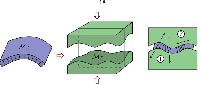
2.2.1 A Physical Interpretation of the Matching Deformation

Consider the first surface to be a thin shell which we press into a mould of the second surface (Fig-ure 2.2). One can distinguish between stresses induced by stretching and compression, and stressed induced by bending that occurs in the surface as it is being pressed. ThusφM can be regarded as

(30)

Figure 2.2:A physical interpretation ofφM as pressing a thin shellMAinto a mould of the surface M_Bbeing matched. The bending (1) and stretching (2) of the thin shell is measured in our matching energy, and minimized by the optimal matchφM.

2.2.2 Measuring Distortion in a Deformation

The distortion in a parameterization was the subject of Section 2.1.2 in the previous chapter, where it was shown that the distortion from the surface patchMonto the parameter domainωunder the inverse parameterizationx−1is measured by the inverse metricg−1∈R2,2. Specifically,ptr(g−1)

measures the averagechange of lengthof tangent vectors under the mapping from the surface onto the parameter plane. Additionally,pdet(g−1₎_{measures the corresponding}_{change of area}_{. We will}

use these quantities in the following sections to account for the distortion of length and area on the surface as we formulate our matching energy in the parameter domain.

The above discussion now applies to the parameter mapsxA andxB of the surfacesMAand MB. We suppose that these parameterizations are defined in an initial step and we assume thatxA andxBas well as the corresponding parameter domainsωAandωB are fixed from now on. Their metrics are denoted bygAandgB, respectively. We will now study the distortion which arises from a deformation of the first parameter domain onto the second parameter domain. First, let us consider deformationsφ :ωA → ωB which are one-to-one. This deformation between parameter domains induces a deformation between the surface patchesφM :MA→ MBdefined by

φM :=xB◦φ◦x−A1.

Let us emphasize that we do not actually expect a one-to-one correspondence between surface patches. Later we will relax this assumption and in particular allow for deformations φ with

φ(ωA)6⊂ωB. The complete mapping is illustrated in Figure 2.3.

(31)

MA

shaded regions of the two surfaces. The partial correspondence is defined on ωA[φ] := ωA∩

φ−1(ωB).

distortion under an elastic deformationφis measured by the Cauchy-Green strain tensorDφTDφ. We wish to adapt this definition to measure distortion between tangent vectors on the two surfaces, as we did with the metricgin Section 2.1.3. Therefore, we properly incorporate the metricsgAand

gBat the deformed position and obtain the distortion tensorG[φ]∈R2,2 given by

G[φ] =g_A−1DφT(gB◦φ)Dφ ,

which acts on tangent vectors on the parameter domain ωA, where products are denoted in ma-trix notation. Mathematically, this tensor is defined implicitly via the identity(gAG[φ]v)·w=

(gB◦φ)Dφ v·Dφ wfor tangent vectorsv, won the surfaceMAand their images as tangent vec-torsDφ v, Dφ wonMB, where here we have identified tangent vectors on the surfaces with vectors in the parameter domains.

As in the parameterization case, one observes thatptr(G[φ])measures the averagechange of lengthof tangent vectors fromM_Awhen being mapped to tangent vectors onM_Bandpdet(G[φ])

measures thechange of areaunder the deformationφM. Thustr(G[φ])anddet(G[φ])are natural

(32)

de-formation,

Ereg[φ] =

Z

ωA

W tr(G[φ]),det(G[φ])pdetgAdξ . (2.7)

This simple class of energy functionals was previously derived in Chapter 2.1 from a set of natural axioms for measuring the distortion of a single parameterization. In particular, the following energy density are typically chosen by the user according to the relative importance of length and area distortion.

2.2.3 Measuring Bending in a Deformation

When we press a given surfaceM_Ainto the thin mould of the surfaceM_B, a major source of stress results from the bending of normals. We assume these stresses to be elastic as well and to depend on changes in normal variations under the deformation. Variations of normals are represented in the metric by the shape operator. We defer the derivation of the shape operatorsSAandSB of the surface patchesM_AandM_B to Appendix B.1, where we end up withtr(SB ◦φ)−tr(SA)as a

measure for the bending of normals. Since the trace of the shape operator is the mean curvature, we can instead aim to compare the mean curvaturehB = tr(SB) of the surfaceMB at the deformed positionφM(x) and the mean curvaturehA = tr(SA)of the surfaceMA. A similar observation was used in [21] to define a bending energy for discrete thin shells. This proposed simplification neglects any rotation of directions due to the deformation,e.g., if the deformation aligns a curve with positive curvature on the first surface to a curve with negative curvature on the second surface and vice versa, an energy depending solely on hB ◦φ−hA does not recognize this mismatch. Nevertheless, in practice the bending energy

(33)

2.2.4 Matching Features

Frequently, surfaces are characterized by similar geometric or texture features, which should be matched properly as well. Therefore we will incorporate a correspondence between one-dimensional feature sets in our variational approach to match characteristic lines drawn on the surface. In par-ticular, we prefer feature lines to points for the flexibility afforded to the user, as well as to avoid the theoretical problems introduced by point constraints [9]. We will denote the feature sets by FMA ⊂ MA and FMB ⊂ MB on the respective surfaces. Furthermore, let FA ⊂ ωA and

F_B ⊂ωB be the corresponding sets on the parameter domains. We are aiming for a proper match of these sets via the deformation,i.e.,

φM(FMA) =FMB

or in terms of differences,FMA\φ

−1

M(FMB) =∅andFMB \φM(FMA) =∅. A rigorous way to

reflect this in our variational approach is with a third energy contribution,

EF[φ] = H1(FMA \φ

−1

M(FMB)) +

H1(FMB \φM(FMA)) (2.10)

whereH1₍_A₎_{is the one-dimensional Hausdorff measure of a set} _A_{on the corresponding surface.}

(34)

localization functions

η(s) = 1 max 1−s ,0

, θ(s) = min s2,1

which act as cut-off functions. For Lipschitz continuous feature sets and bi-Lipschitz continuous deformations, we observe thatE˜_F[φ]→ EF[φ]as→ 0, which motivates our approximation. In

view of the later discretization, we can reformulate the second term in (2.11) as

Z

Usually, we cannot expect that φM(MA) = MB, particularly near the boundary where certain subregions of M_A will have no corresponding counterpart on M_B and vice versa. Therefore, we must allow for points onMB with no pre-image inMAunder a matching deformation φM,

and points onM_Awhich are not correlated to points on M_B viaφM (cf. Figure 2.3). Thus we

must adapt the variational formulation accordingly. Ifφ(ωA) 6= ωB, thenφM is now defined on xA(ωA[φ])only, where

ωA[φ] :=φ−1(φ(ωA)∩ωB)

is the corresponding subset of the parameter domainωA. Furthermore, we define new energies (with modifications marked in red):

For an energy that controls tangential distortion, it is still helpful to control the regularity of the deformation outside the actual matching domainωA[φ], where we would like to allow significantly larger deformations by using a “softer” elastic material. Hence we will suppose thatgB, which is initially only defined onωB, is extended toR2and takes on values that are relatively small to allow

for greater stretching.

(35)

variable boundary∂ωA[φ]will appear. Since these are tedious to treat numerically, we will rely on another approximation for the sake of simplicity. Our strategy here is to change the domain of integrationωA[φ]to a superset ω which extends beyond the boundary∂ωA[φ]. Doing so means that special treatment of boundary integrals is no longer necessary, although we are now required to evaluate the integrands of the energies outside ofωA, and similarly for deformed positions outside ofωB. To achieve this, we will extend our surface quantities ontoω\ωAandω\ωB, respectively, by applying a harmonic extension with natural boundary conditions on∂ωtogA, gBandhA, hB (e.g., we definehA as the solution of Laplace’s equation on ω\ωA with vanishing flux on∂ω). Additionally, we introduce a regularized characteristic function

χA(ξ) = max(1−−1dist(ξ,A),0) (2.14)

to cause the energy contributions to be ignored at some distanceaway fromωA[φ]. Thus, instead of dealing with a deformation dependent-domainω[φ]in the definition of our different energy con-tributions, we always integrate over thewhole image domainω and insert the product of the two regularized characteristic functions

χ(ξ) =χ_ω_A(ξ)χ_ω_B(φ(ξ))

as an additional factor in the energy integrand. We apply this modification to the energyEbend(2.9) and the already regularized energyE˜_F (2.11) and denote the resulting energies by

E_bend and E_F , (2.15)

respectively.

2.2.6 Definition of the Matching Energy

We are now ready to collect the different cost functionals and define the global matching energy. Depending on the user’s preference, we introduce weightsβbend, βreg, βF for the approximate

en-ergies in (2.15) — we have found thatβbend= 1, βreg = 0.01, βF = 5work well — and define the

global energy

(36)

which measures the quality of a matching deformation φ on the domainω. Finally, in the limit

→0we obtain a weighted sum of (2.7), (2.12) and (2.13):

E[φ] =βbendEbend[φ] +βregEreg[φ] +βFEF[φ]. (2.17)

(37)

Chapter 3

Algorithms

(38)

3.1

The Parameterization Algorithm

We shall now describe our algorithm to construct an optimal parameterization for a discrete surface patch. We assume that the surface patchMis provided as a manifold triangle mesh with boundary. A discrete parameterization x : ω → M is a piecewise-affine mapping on the triangles in the parameter domainω⊂R2to the corresponding triangles inR3. The algorithm generates an optimal,

discrete deformationφ˜:ω→_R2_{which we apply directly to the planar triangulation}_ω_{to obtain the}

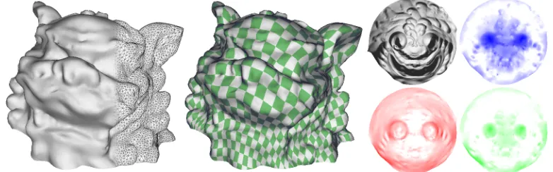
optimal parameter domainω[ ˜φ] := ˜φ(ω)(cf. Figure 2.1). The final parameterization is fully defined by the coordinates assigned to the vertices of the triangles inω[ ˜φ](e.g., as “texture coordinates” for texture mapping, Figure 3.1).

Figure 3.1: For a surface mesh (left, 36k triangles), a parameterization is computed, depicted through a texture map (middle). The parameter domain (right) is optimized through the minimiza-tion of energy funcminimiza-tions which control length, area and angle distorminimiza-tion (shown clockwise from top right; dark regions indicate higher energy).

The user controls the parameterization through the choice of parametersα = (αl, αa, αc)that balance the trade-off between length, area and angle distortion, respectively. For example, specify-ing a larger value forαawill result in a parameterization that is biased toward low area distortion at the expense of greater length and angle distortion,etc.The parameters must satisfy the conditions stated in (2.6), namely

αl>0, αa>0, αc ≥0.

(39)

We will now turn to the main steps in the algorithm:

1. Construct an initial parameterization of the surface.

2. Optimize the parameterization through a discrete deformation of the parameter domain that minimizes the energyE[·]defined in (2.5).

3.1.1 Initial Parameterization

Our algorithm requires that an initial parameterization be provided for the subsequent optimization of the parameter domain. With this optimization step in mind, we desire an initial parameterization that is close to optimal to make the energy minimization more efficient. It follows that this parame-terization should already have low distortion. Moreover we advocate choosing an initial parameter-ization with natural boundary conditions over a constrained boundary,e.g., a convex polygon in the plane. In the latter case one often encounters extreme shearing and compression in the boundary elements which is difficult to correct through numerical optimization.

For this purpose we use the natural conformal map [15] in our examples (also known as the least-squares conformal map [29]). This parameterization has low angle distortion and natural boundary conditions, and is cheap to compute since it only requires the solution of a sparse linear system. Other free-boundary parameterization algorithms can be used (e.g., [26, 46]) provided that the initial parameterization is admissible (cf. Section 2.1.2).

Recall from Section 2.1.5 that the energy (2.5) is a function of the principal invariants of the inverse metric g−1. On inspection only the conformal (third) term in the energy is unaffected by uniformly scaling the surface patchMor the parameter domainω. In practice we would like the parameterization energy to be scale-invariant. In many applications the scale of the ambient space in R3 and the parameter space in R2 are chosen independently and therefore a parameterization

(40)

for any isometric parameterization of a developable surface. When the optimal parameterization is constructed, the parameter domain is returned to its original scale using the inverse scale factorσ−1.

3.1.2 Finite Element Discretization

Suppose that ω is an admissible triangle mesh in the parameter space R2, and letT denote the

triangles ofω. A discrete deformationφ:ω →R2 is a vector-valued function, whose components

are piecewise-affine, continuous functions. For these deformations we have to evaluate the discrete counterpart of energy functional (2.5),

E[φ] = X

T∈ω

W tr(C[φ]),det(C[φ])pdetg|T|

with the area of a triangle in the plane denoted by|T|. On each triangleT ∈ω, a constant Cauchy-Green strain tensor is defined byC[φ] := Dφ g−1DφT where the derivativeDφand the discrete metricgare constant matrices inR2,2.

Besides evaluating the discrete energy for a given deformationφ, we have to compute the gra-dient ∇E[φ] and (optionally) the Hessian ∇2_E_[_φ_] _{in the actual minimization algorithm in}

Sec-tion 3.1.3, which requires the differentiaSec-tion of the discrete energy with respect to the discrete de-formation. All the necessary expressions to assemble these matrices are provided in Appendix B.2. A necessary condition for a discrete deformationφto minimize the energy is∇E[φ] = 0. Due to our assumption of frame indifference (2.2) the energy is invariant under Euclidean motion. To remove these degrees of freedom we add two constraints on the zero momentM0(φ) to eliminate

translations, and one on the angular momentumM1(φ)to cancel rotations:

M0(φ) :=

(41)

Instead of solving∇E[φ] = 0forφone now solves the equation∇E¯[φ] = 0for the deformationφ

and the Lagrange multipliersλ1, λ2, λ3. To find the minimum of this energy with a Newton method

one also needs the Hessian. Based on∇2_E_[_φ_]_{we obtain}

where mis the vector of masses of the nodal basis functions, i.e., mk := P

Nk 1₃|T|with Nk

denoting the set of triangles incident to vertex k = 1,· · ·, n. Note that while this new Hessian ∇2_E¯_[_{φ, λ}_]_{is not positive definite, it does not pose a problem for our algorithm as we explain below.}

3.1.3 Numerical Optimization

We use an iterative approach to find a sequence of discrete deformations{φi}i=0···N such thatφN minimizes the discrete energyE[·], i.e., E[φ0] > E[φ1] > · · · > E[φN]and∇E[φN] = 0. The optimal deformationφ˜=φN thus generates the final, optimal parameterizationx[ ˜φ] :=x◦φ˜−1.

Because our energy is polyconvex, it has multiple local minima and therefore it is non-trivial to guarantee that one will find a global minimum. Our strategy is to find a local energy minimum starting from a reasonable initial guess, namely, the initial parameterization in Section 3.1.1. It follows that the minimizing sequence of deformations begins withφ0being the identity function.

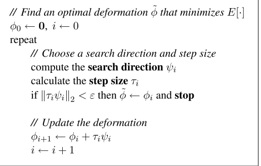
// Find an optimal deformationφ˜that minimizesE[·] φ0←0, i←0

repeat

// Choose a search direction and step size

compute thesearch directionψi

(42)

We use a simple line search method to find φ˜(Figure 3.2). Each iteration of the line search computes a search directionψi and then decides how far to step in this direction. The iteration is given by

φi+1 ←φi+τiψi

Many classical numerical methods can be used to computeψi (Figure 3.2,search direction). There is a typical trade-off between performance, in terms of the number of iterations to converge to the minimum, and the complexity of algorithm, which is related to what local model of the energy landscape is used in selecting the search direction. For example, the simplest gradient descent method relies only on the local gradient,i.e.,ψi =∇E[φi], but it has poor convergence properties. We chose to use a Newton method in our implementation because it guarantees a quadratic rate of convergence close to an optimal solution (Chapter 3, [38]). It computesψiby solving a sparse linear system,

saddle-point problem (3.1), one could apply Uzawa’s algorithm [8]. We simply use a precondi-tioned conjugate gradient algorithm. We have never observed any difficulty in practice even though theoretically the matrix∇2_E_¯_[_φ

i, λ]is not positive definite. As a preconditioner, we apply a diagonal preconditioning to∇2_E_¯_.

The next step is to determine the step sizeτifor the iteration (Figure 3.2,step size). We require

τi to be chosen such that the energy decreases at each iteration. We accomplish this with a simple step size control algorithm that uses the Armijo condition [38] to guarantee sufficient decrease of the energy functional (Figure 3.3). The parameters control how aggressively the algorithm is in taking large steps — we find thatτi = 1, ρ= 0.8, c= 0.5work well in practice.

// Chooseτi >0, ρ, c∈(0,1)

repeat untilE[φi+τiψi]≤E[φi] +cτi∇E[φi]Tψi

τi ←ρ τi

(43)

Beside asking for sufficient decrease of the energy, one must be concerned with taking legal

steps. Our concern lies in the fact that an illegal step φi +τiψi that generates an inadmissible deformation could actually lower the energy. This problem can be seen directly from our energy functional (2.5). If a triangle elementT reverses its orientation due to a fold in the deformation, one can experience a negative energy value. One can address this issue by defining E[φ] to be unbounded fordetφ <0, which is a natural extension ofE[·]sinceE[φ]→ ∞asdetφ→0. This is equivalent to simply disallowing a step for whichdet(φi+τiψi)≤0on any triangleT.

We stop the line search method when the update is sufficiently small in theL2norm, controlled by the threshold parameterε > 0 (Figure 3.2, stop). If we have reached a local minimum, i.e., ∇E[φi]≈0, then we have achieved the optimal deformationφ˜=φi.

The line search will also terminate if no further progress can be made to reduce the energy. This “locking” can occur when the line search gets lost in the energy landscape because of a poor choice for the initial parameterization. In this case, a simple continuation method on the energy parameters

αcan be used to set up a series of easier optimization problems,

H(φ, θ) =E[φ]|_α₌₍₁₋_θ₎_α0₊_θα1

where the blend parameterθ∈[0,1]is chosen from a monotonically increasing sequence{θj}j=0···J that transforms the energy landscape from E[·]|α0 to the desired energy E[·]|α1. The motivation comes from choosing α0 so that the initial parameterization is close to an optimal solution of

E[·]|α0 = H(·, θ0). The minimizer ofH(·, θj)is used as the initial parameterization for the next problem in the sequence, H(·, θj+1). Thus by completing this sequence one obtains the optimal

(44)

3.2

The Matching Algorithm

In Chapter 2.2 we developed a variational framework for matching surface patches without regard to a particular discretization. Now we will describe our method for constructing a match based on a straightforward discretization using finite elements. We assume that the surface patchesM_A and MB are given as triangle meshes. In the initial step, we generate parameterizations which define triangulated parameter domains ωA and ωB using the approach described in Section 3.1. Because of the difficult algorithmic details, we do not wish to deal with effectively overlaying two triangulations during the numerical solver stage. Consequently we discretize the domain onto a regular grid (“image”) and evaluate the associated surface quantities needed in the energies at each pixel (in effect we may think of this as a geometry image [22]).

This setup has two principal advantages: (1) the resolution of the original meshes is decoupled from the resolution used in the image domain and (2) multiscale algorithms are far simpler to im-plement in the regularly sampled image grid than over arbitrary triangle meshes (even if flat). In particular, we can use higher sampling rates in the image domain to alleviate aliasing problems. Ad-ditionally, the image pyramids used by a hierarchical solver have far more efficient memory access patterns on modern processors than one achieves with arbitrary meshes.

We now turn to the basic components of the implementation:

1. Construct parameterizations for the surface patches.

2. (optional) Select matching features on the surfaces with separate texture maps.

3. Evaluate the metric and mean curvature by scan converting the surface triangulation in the parameter domain.

4. Apply a finite element discretization and optimize the matching deformation using a multiscale approach to minimize the energyE[·]defined in (2.16).

3.2.1 Surface Patch Parameterization

(45)

(46)

in Section 3.1 to parameterize the surfaces. In practice, we find that αl = αa = αc = 1₃ works nicely for this purpose.

Once both surfaces have been parameterized, we perform a rough alignment by applying a normalizing transformation such that the parameter domains are subsets of the domainω:= [0,1]2. Due to the feature energy contribution from (2.11) and the hierarchical nature of the minimization algorithm this rough alignment is entirely sufficient.

3.2.2 Feature Set Construction

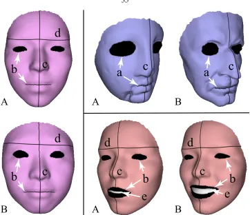
The user can control the match by identifying sets of similar features on the surface patches. The cost functionalE_F[·]from (2.11) helps to guide the energy minimization to match the corresponding features. Marking the desired feature setF_A is most easily accomplished in the image domains. Figure 3.5 gives examples of these, showing the texture images mapped onto the surfaces. The actual feature sets are the boundaries of the (pixel) regions drawn by the user on the texture image. Note that when we match features, we donotconstrain points since this would break the regularity of the deformation. Instead, we match feature curveswhich permits sliding of the deformation along the curve.

There are many ways in which features can be used to control a match:

Coarse control of the match is achieved by roughly selecting corresponding geometric features and gradually decreasing βF to zero as the multiscale method goes to finer resolutions

(Fig-ure 3.5a).

Precise control over matching texture features (e.g., on the face,etc.) is achieved by selecting the corresponding pixels in the feature set image (Figure 3.5b).

Lines of symmetry drawn as features allow deformations tangential to the feature boundary, but prevent deformations that are transverse to it (Figure 3.5c).

(47)

a

Figure 3.5:Examples of user-defined feature sets: (a) coarse registration of geometric features; (b) aligning texture features; (c) lines of symmetry; (d) preventing smooth, rigid regions from sliding; and (e) increasing the elasticity of highly deformable regions.

The distance maps used in the definition of the feature energy are discretized by an upwind scheme for the corresponding Eikonal equations [40] (Figure 3.6c). We used the particular upwind finite element algorithm of Bornemann [6] since it fits well with our overall finite element frame-work. Multiple sets of overlapping features are accounted for by taking the distance to the nearest feature to create a single distance map.

3.2.3 Evaluation of Surface Properties

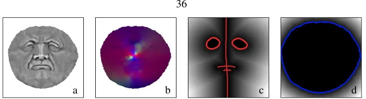
The matching energy needs to evaluate surface quantities such as the mean curvatureshA, hB, met-ric tensorsgA, gB, distance to the feature setsFA,FB, and signed distance to the domain boundaries

(48)

a b c d

Figure 3.6:Surface properties are evaluated once and rasterized into images for (a) mean curvature hA; (b) the metric tensorgA, with components shown as rgb values; (c) the distance map for the

feature setFA, shown in red; and (d) the distance map for the characteristic functionχ_A, with the

domain boundary∂ωAin blue.

ForhAwe use the magnitude of the mean curvature normal [16, 34]. The sign is chosen accord-ing to the surface normal, which we take to be the area-weighted sum of triangle normals around a vertex. Other measurements for the mean curvature would work equally well (see [34] for a sur-vey). Since gA is symmetric and constant over each triangle element, we can evaluate its three unique components as a function of the triangle vertices. The calculation of the Jacobian of the pa-rameterization over a triangle is well documented in the papa-rameterization literature (e.g., see [44]). The distance map forFAis described above and illustrated in Figure 3.6c. To compute the distance map for the characteristic function, we rasterize the domain ofM_A and then generate its signed distance field in a similar manner toFA(Figure 3.6d).

3.2.4 Multiscale Finite Element Method

The total energyE[·]is highly non-linear. In particular the bending energy causes many local min-ima in the energy landscape over the space of deformations. We take a multiscale approach, solving a sequence of matching problems from coarse to fine scales. This type of method is frequently applied and well understood in image processing [2], allowing for a robust and efficient global minimization on complicated energy landscapes (Figure 3.7).

To begin, let us define a sequence of energies(Eσk₎

k=0,···,mcorresponding to scale parameters

(49)

// Build the image pyramid

fork=mdownto0do

filterimages at levelkusingσk

// Optimizeφkfrom coarse to fine scales φ0_←₀

fork= 0tomdo

minimizeEσk _{starting with}_φk

ifk < mthenprolongateφk_to_φk+1

Figure 3.7:Pseudo-code for the multiscale algorithm.

on levelkwith a deformationφk_{, this deformation is already in the contraction region of the global} minimum on the next finer scalek+ 1(Figure 3.7,prolongate). The prolongation ofφktoφk+1is performed using bilinear interpolation.

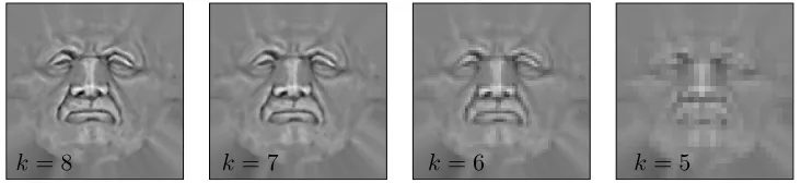
k= 8 k= 7 k= 6 k= 5

Figure 3.8:The mean curvature functionhAis extended to the full image domainωand successively

restricted to coarser gridsk= 8,· · · ,0from the multigrid pyramid.

It remains for us to define the scale of energies. First, we replace the functions on the surfaces as they appear in the different energy functionals by pre-filtered, smoothed representations (Figure 3.7, filter). A Gaussian filter of width σk is used to define the smoothing on the surfaces MA and MB. Exploiting the connection between Gaussian filtering and the fundamental solution of the heat equation, we replace the mean curvatureshA andhB (appearing in the bending energy) by pre-filtered mean curvature functionshσk

A andh σk

B. This amounts to applying the appropriate filter kernels to the correspondinghA andhBimages. Figure 3.8 shows images representing a scale of filtered mean curvature functions hσk

A on the parameter domain of a surfaceMA. Similarly, we filter the metric tensorsgAandgBcomponent-wise.

The regularization parameterin the definition of the energies also depends on the sequence of scale parameters and is set to(σk) = 2σk. For the matching problems considered in this paper, we start withσ0 = 1, and defineσk = 1₂σk−1 fork = 1,· · · m. In our examples the parameter

(50)

Chapter 4

Analysis

(51)

4.1

Surface Parameterization

The following provides demonstrations of the parameterization algorithm in Section 3.1. These feature typical but nonetheless challenging examples of parameterizations aimed at measuring the performance of our method. Fundamentally, we expect that the parameterizations generated for discrete surfaces uphold the principles that we established in our variational model for continuous surfaces (cf. Section 2.1). The central tenet is the existence of a continuous and locally bijective parameterization that is optimal for a given set of parametersα= (αl, αa, αc), which is summarized in Theorem 2.2. Moreover, the parameterization should be robust subject to different triangulations of the surface geometry, due to the finite element discretization of the parameterization energy in Section 3.1.2. Finally, we expect the distortion in the parameterizations to be distributed in relative accordance with the user’s choice of parametersα. The following examples show that all of these requirements are satisfied in our implementation.

4.1.1 Convergence of the Optimization Algorithm

For global energy minimization methods one is typically concerned with the rate of convergence to an optimal solution (if convergence occurs at all) and the number of iterations spent in the min-imization algorithm. Figure 4.1 plots the energy decay for a series of examples, in which a quasi-conformal initial parameterization due to [15, 29] is optimized based on our own nearly quasi-conformal energy (αc αl, αa). The vertical axis measures theL2norm of the energy gradient on a logarith-mic scale,i.e.,log10 k∇E[·]k2

. The trend of these graphs shows that when the deformationφiis sufficiently close to the optimal solution, the Newton method achieves its optimal quadratic rate of convergence. In all of these examples the maximum step size (β = 1) was chosen at each iteration which further supports the choice of a Newton method for our problem.

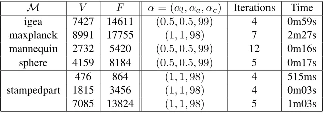
M V F α= (αl, αa, αc) Iterations Time

(52)

1 2 3 4 5 6 7 8 9 10 11 12 1 2 3 4 5 6 7 8 9 10 11 12

Figure 4.1: Plots of the energy decay for the sequence of deformations computed in the parame-terization energy minimization algorithm. A quadratic rate of convergence is experienced near the optimal solution.

We can take a closer look at this process by inspecting the intermediate parameterizations that are generated during the minimization. Due to the invariants of our algorithm, these parameteri-zations are guaranteed to be admissible. Figure 4.2 depicts the intermediate deformations acting on a rectilinear grid in the initial parameter domain ω. Notice that much of the optimization is involved in improving the area distortion of the initial parameterizations. Since solutions of the natural conformal parameterization do not have direct control over the area factor, this result is not surprising. The final, optimal deformation is aM¨obius transformationsince the conformality of the parameterization is preserved under this mapping.

(53)

(a) i= 1 i= 2 i= 3 i= 4

(b) i= 3 i= 6 i= 9 i= 12

Figure 4.2: A sequence of deformations is generated by the global energy minimization algorithm, shown here acting on a grid in the parameter domain for (a) the stamped mechanical part and (b) the mannequin.

4.1.2 Convergence of the Continuation Method

The energy landscape that expresses the relationship between the initial parameterization and the optimal parameterization can be very complex: since the parameterization energy is polyconvex, it contains many local minima. Global optimization methods perform quite well when the initial parameterization is sufficiently close to the optimal solution, but they can quickly break down if a global minimum is nowhere in sight.

Continuation methods provide a strategy to gradually change the energy landscape allowing one to transform the optimal parameterization for one set of parameters α0 to the solution for a

second parameter setα1 (cf. Section 3.1.3). Our strategy is quite na¨ıve: after finding the optimal

parameterization for the energy corresponding to parametersα0, we use this solution as the initial

parameterization for the optimization of the energy defined byα1. Table 4.2 lists the number of

iterations and the execution time for the optimization ofE[φ]|α1, starting from a parameterization

˜

φthat minimizes E[·]|α0 (cf. Table 4.1). Although our continuation method is simple, it proves to be entirely effective. One can often take large steps betweenα0 andα1 in the continuation method

(54)

M α0 α1 Iterations Time

igea (0.5,0.5,99) (33.3,33.3,33.3) 6 0m54s maxplanck (1,1,98) (33.3,33.3,33.3) 16 3m56s sphere (0.5,0.5,99) (99,0.5,0.5) 7 0m25s

(0.5,0.5,99) (3,3,94) 10 0m10s mannequin (90,5,5) (20,20,60) 12 0m12s

(60,20,20) (33.3,33.3,33.3) 5 0m05s

Table 4.2: Performance figures for optimal parameterizations obtained using the continuation method. The iterations refer to the steps taken in the energy minimization ofE[·]|_α1, starting from an initial parameterization that minimizesE[·]|_α0.

4.1.3 Robustness to Surface Discretization

The continuous energy model that we use has several distinct advantages. Since our energy is defined in the continuous setting, the solution to the minimization problem is insensitive to the particular discretization of the surface. This fact can be observed because different discretizations minimize consistent approximations of the same continuous energy functional. In Figure 4.3, we consider the successive refinement of a triangular grid that represents a stamped mechanical part. Notice how the parameterization converges rapidly, and its main features are apparent even at the coarsest resolution. Not surprisingly, the number of Newton steps taken for each of these examples is nearly identical (cf. Table 4.1).

(55)

®=(.01,.01,.98) _®₌(.49,.02,.49) ®=(.98,.01,.01) _®₌(.49,.49,.02) ®=(.01,.98,.01) _®₌(.02,.49,.49) [3,4]

10 1

Angle Distortion

100 Area Distortion

10

1 ₁₀₀

Length Distortion

10

1 ₁₀₀

Figure 4.4: The parameterization is controlled by parameters α = (αl, αa, αc)which capture the

trade-off between length, area and angle preservation, respectively. Texture maps of the initial parameterization on the left and solutions for different parameter settings are shown on top, with the parameter domain beneath. A plot of the maximum, minimum and mean distortion is shown below. Notice that the measured distortion tends to reflect the trade-offs in the choice of parameters.

®=(.005,.005,.99) ®=(.005,.99,.005) ®=(.99,.005,.005)

(56)

4.1.4 Distortion in Optimal Parameterizations

Figure 4.4 demonstrates our algorithm for a variety of parameter values. Given the initial parameter-ization on the left, each parameterparameter-ization on the right is obtained by minimizing the corresponding energy. The relative importance of the three competing parameters αl, αa, αc is reflected in the distortion of the final parameterization. Recall that distortion can be measured as a function of the maximum and minimum eigenvalues Γ, γ of the first fundamental form of the parameteriza-tion funcparameteriza-tion. We calculate the mean distorparameteriza-tion for a parameterizaparameteriza-tion as the arithmetic sum of the contributions from each triangle in our discretization. Popular measures of distortion for angles (pΓ/γ), area (√Γγ) and length (√Γ +γ) for Figure 4.4 are reported in the bottom graphs, where the extreme deformations in the parameterization functions clearly show the trade-offs between the different distortion measures. This correspondence is further explored in Figure 4.5, which demon-strates the effect of minimizing the different energy terms on parameterizations of a sphere that has been cut.

4.1.5 Comparison to Related Work

We have presented a parameterization method that gives the user flexible control over the trade-off between area, length and angle distortion. Figure 4.4 demonstrates this control with examples that range from angle preserving to area preserving, and a comprehensive balance with length distortion

(a)

(57)

in the rest. This contrasts our method from previous work, which largely focused on optimizing for only one measure of distortion, or possibly using linear combinations of energies. Figure 4.6 demonstrates that this trade-off is highly effective. For example, wh