Automatic Climate Classification of Environmental Science Literature

Automatic Climate Classification of Environmental Science Literature

♠Department of Computing and Information Systems ♥NICTA Victoria Research Laboratory

♦Department of Resource Management and Geography The University of Melbourne, VIC 3010, Australia

[email protected], [email protected], [email protected], [email protected]

Abstract

Climate type is one of the potentially most relevant pieces of metadata for identify-ing studies in evidence-based environmen-tal management. In this paper, we pro-pose a method for automatically predict-ing the climate type in environmental sci-ence literature using NLP techniques, rel-ative to a pre-existing set of climate type categories. Our main approaches com-bine toponym detection and resolution us-ing two different resources with support vector machines. The results show great promise, but also further challenges, for using NLP to extract information from the vast and rapidly growing collection of en-vironmental sciences literature.

1 Introduction

In this paper, we investigate the task of automatic prediction of climate type (e.g.temperateorarid) in environmental science abstracts. The climate type of an environmental science study is crucial information, which gives context to the research and insight into its wider implications and applica-bility. Availability of climate information as meta-data has clear value to researchers performing a systematic review of the literature or comprehen-sive analysis of the evidence. However, the man-ual annotation of climate type over a large volume of literature is a time-consuming task. In this pa-per, we seek to automate the climate annotation process with natural language processing (NLP) techniques. The task of climate type classification is complex as although the label set is relatively small, the geographic granularity is fine and to-ponym ambiguity becomes a significant problem — toponyms commonly mentioned in the envi-ronmental sciences (e.g.Murray River) are often large and cover multiple climates, which presents

difficulties for a point-based representation of to-ponyms. Initially, experiments are run to exam-ine the effectiveness of the direct application of the classifiers developed by Willett et al. (2012) for study region classification. We then investigate methods for adapting these techniques to the cli-mate task through the modification of the toponym resolution component of our classifiers. These ap-proaches include utilizing a K¨oppen-Geiger cli-mate classification world map to resolve toponyms to climate instead of region, in addition to exper-iments with targeting types of toponyms reliable for identifying climate.

2 Related Work

The methodology used to extract and disam-biguate toponyms is based on a standard approach to geographic information retrieval, which was presented, e.g., by Stokes et al. (2008) in their study on the performance of individual compo-nents of a geographic IR system. In particu-lar, the named entity recognition and classifica-tion (NERC) and toponym resoluclassifica-tion (TR) com-ponents are the basis for the main classifiers in this study.

The unique opportunities and challenges spe-cific to retrieving geospatial information have been well documented, particularly in the context of geospatial information retrieval where queries and documents have a geospatial dimension (San-tos and Chaves, 2006). Aside from finding loca-tions in the text, the disambiguation of what exact location a term in a text is referring to presents a unique challenge in itself, and a variety of ap-proaches have been suggested and demonstrated for this task (Overell and R¨uger, 2006).

identi-fications of locations, prominence in Wikipedia, and population statistics.

As a specific instance of toponym resolution over environmental sciences data, Willett et al. (2012) proposed a method for predicting the “study region” of a published abstract, based on text categorisation techniques using features in-cluding frequency distributions of resolved to-ponyms and a bag of word unigrams. Their best method was able to determine the study region with an accuracy of 0.892, combining toponym resolution from DBpedia and GeoNames with the bag-of-toponyms features. We adapt this method to climate type classification, and present details of the method in Section 5.

This work is inspired in part by work on ev-idence based medicine (EBM). As Sackett et al. (1996) define it: “Evidence based medicine is the conscientious, explicit, and judicious use of cur-rent best evidence in making decisions about the care of individual patients.” The reasons for mov-ing towards an evidence-based model of environ-mental management have obvious parallels to the motivation for the practice of EBM. Although the structure of evidence will differ between the do-mains, many of the techniques applied in research for EBM are likely to have application for our cur-rent task. Successful applications of NLP to EBM include sentence categorization for information on randomized controlled trials (Chung, 2009; Kim et al., 2011), the labelling of sentences with “PICO” (Patient/Problem, Intervention, Comparison and Outcome) labels to aid clinical information re-trieval (Boudin et al., 2010), and the automatic assignment of Medical Subject Headings (MeSH) terms to PubMed abstracts (Gaudinat and Boyer, 2002).

3 Resources

In this section, we provide details of key resources used in this paper, namely:

• Eco Evidence, a manually-curated database of metadata for environmental science litera-ture, which provides the basis of the data used in our experiments

• DBpedia and GeoNames, as resources for to-ponym resolution

• the K¨oppen-Geiger Climate Map of Peel et al. (2007)

3.1 Eco Evidence

Eco Evidence (Webb et al., 2011) is a tool for liter-ature review and evidence synthesis, consisting of two parts. The first is the underlying Eco Evidence Database (EED) (Webb et al., 2012a), in which the evidence items are stored. The citations for envi-ronmental studies are catalogued in the database as separate entities, and evidence items may be stored by means of linking them to the citation for the study from which the information came. Addi-tional details about the study’s location, scale and ecosystem can also be stored with each citation to aid the process of filtering relevant evidence. An example of a record in the EED is given in Fig-ure 1. The database is in active use in a number of research projects currently, and evidence therein has also formed the basis of several published sys-tematic reviews (Webb et al., 2012b).

The Eco Evidence Analyser (EEA) retrieves the potentially relevant evidence from the EED for a hypothesised cause and effect, then weights and analyses the selected evidence to determine whether there is adequate evidence to support or reject the hypothesis. For the Eco Evidence Anal-yser to be effective, the underlying EED must contain as much evidence as possible. However, the database has to date been populated through manual annotation of citations with their evidence items, which is a time-consuming process (Webb et al., 2012b). Our work is motivated by the possi-bility of streamlining the population of the EED, by automatically extracting climate information, but potentially in the future extending NLP-based extraction to other evidence items.

3.2 Toponym Resolution

Toponym resolution is a key component of our experiments, and we worked with two different resources in disambiguating toponyms: DBpedia and GeoNames.

DBpedia (http://www.dbpedia.org) is a database of structured content extracted from Wikipedia. We utilize DBpedia as a source of in-formation for resolving ambiguous toponyms by finding the DBpedia pages for likely candidates based on the toponym name, and extracting geo-graphic coordinates to identify their location. For terms with multiple meanings, DBpedia will con-tain a disambiguation page. We use the disam-biguation page in one of two ways:

Figure 2: World map of K¨oppen-Geiger climate classification.

result is returned; in the event that coordi-nates are unavailable for the first possibility on the disambiguation page, no resolution is recorded for the term.

2. the top-5 approach: up to the top-5 results are used to represent a given toponym

Another tool we use for toponym resolution is GeoNames (http://www.geonames.org), a gazetteer which is based on data from a wide variety of sources. A toponym query via the GeoNames search API provides a ranked list of geospatial results, each of which is linked to in-formation such as geo-coordinates, and the popu-lation of towns/cities.

3.3 K¨oppen-Geiger Climate Map

We map geographic coordinates from DBpedia to a world map of K¨oppen-Geiger climate classifica-tion (Peel et al., 2007). The K¨oppen-Geiger cli-mate classification system divides clicli-mates into five main groups, as detailed in Figure 2 (with each climate type represented by subclasses of the prefix indicated in parentheses): Tropical(“A*”),

Arid(“B*”),Temperate(“C*”),Cold(“D*”) and

Polar(“E*”).

4 Dataset

The dataset used in our experiments was sourced from the collection of 3977 titles and abstracts from the Eco Evidence database, each of which has been manually annotated with a climate type. The climate types are made up of 5 basic types — Temperate,Tropical,Dry, Polar andAlpine

— in addition toMultiple (i.e. multiple basic cli-mate types, without specification of which specific types) and Other. Eco Evidence does not cap-ture information on which basic classes make up a Multiple label, so we are not able to treat the problem as a multi-label classification task. In-stead,Multipleis represented in the same way as the basic classes. Note the slight mismatch with the climate types used in the K¨oppen-Geiger cli-mate classification.

The Eco Evidence dataset is quite unbalanced, as detailed in Table 1: Temperateis the majority class by a very large margin, andPolarandOther

are very small minority classes.

5 Methodology

Climate EU AU AF AN AS NA SA OC MU OT TOTAL

Temperate 768 390 46 0 98 1055 9 98 13 1 2478

Tropical 1 102 45 0 65 51 98 10 7 1 380

Dry 9 89 67 0 21 162 7 0 1 0 356

Polar 2 0 0 1 0 5 1 1 2 0 12

Alpine 139 1 0 0 39 278 3 0 1 2 463

Multiple 22 24 9 0 13 102 1 1 113 1 286

Other 0 1 0 0 0 1 0 0 0 0 2

TOTAL 941 607 167 1 236 1654 119 110 137 5 3977

Table 1: Distribution for the gold standard climate classifications across the gold standard study region classifications (EU = Europe, AU = Australia, AF = Africa, AN = Antarctica, AS = Asia, NA = North America, SA = South America, OC = Oceania [other than Australia], MU = Multiple, OT = Other; the boldfaced number indicates the majority-class for a given continent)

(2012). First, the Stanford Named Entity Recog-niser (Finkel et al., 2005) is used to identify location-type NEs in each abstract. Each NE is then mapped to a set of toponyms, based on DB-pedia or GeoNames, and the counts of toponyms are aggregated into bag-of-toponyms (BoT) fea-tures. Finally, a linear-kernel support vector ma-chine (SVM) is used to train a supervised classi-fier.

We experiment with both: (1) study region clas-sification (at the continent level), and a majority-class majority-classification for that continent; and (2) re-placement of continent-level classes from the orig-inal paper with climate-based classes. In the latter case, the toponyms are resolved to climates using the K¨oppen-Geiger climate classification system. One issue that arises with the use of the climate map is that the classifications of the climate map do not all directly correspond to labels used in the dataset. Temperate,TropicalandPolarhave di-rect matches, but the climate map classesColdand

Ariddo not. These two labels were mapped to the

AlpineandDrylabels respectively for the bench-mark system. Note that this is only relevant for the majority-class classification; in the case of the to-ponym resolution, the supervised classifier is able to learn its own mapping between the K¨oppen-Geiger climate classification system and the 5+2-class climate system used by Eco Evidence.

We also include structured features. That is, separate frequency distributions of the number of tags resolving to each climate type are used for each zone of the abstract, based on partitioning the abstract into 4 equal-sized zones (based on word count). Each of these frequency distributions are treated as separate vectors of unique features. The

title of the paper is treated as an additional fifth zone and feature vector.

We also present a majority class baseline, that selects the majority climate type from the train-ing data (Temperate). In addition, we experi-ment with taking a majority vote across the climate type(s) that each toponym in the abstract resolves to.

Subsequent experiments attempt to target only toponyms more likely to reliably identify cli-mate. This was done by excluding toponyms of the GeoNames feature code “A”, which idtifies countries, states, regions, and similar en-tities.1 These experiments are only completed with the GeoNames multiple result classifiers, as no reliable method of identifying the form of to-ponym is available in DBpedia. These experi-ments are performed based on the hypothesis that the point-based representation of coordinates ex-tracted from GeoNames for these coarse-grained toponyms may prove problematic, as larger areas are more likely to contain more than one climate type. Precision may therefore be enhanced by fil-tering these toponyms out.

For all classifiers, we evaluate our model with classification accuracy, measured using 10-fold stratified cross-validation over the full dataset. As our learner, we use LIBSVM with a linear kernel (Chang and Lin, 2011).

6 Results

We first present results based on the methodology of Willett et al. (2012) for classifying study region, simply mapping toponyms onto continental study

Classifier Accuracy

Zero-R 0.623

Bag-of-Toponyms (BoT) 0.681

Bag-of-Words (BoW) 0.654

BoT + BoW 0.659

DBpedia + GeoNames top result (“dbp+Geo:TR”) 0.623

dbp+Geo:TR + BoT 0.681

dbp+Geo:TR + BoW 0.681

dbp+Geo:TR + BoT + BoW 0.687

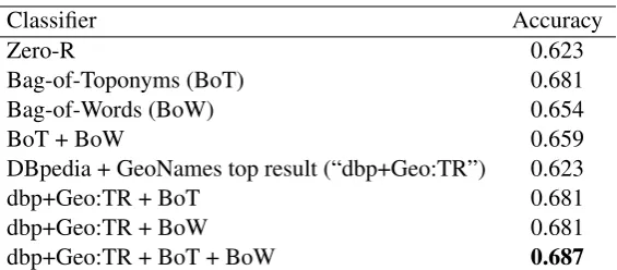
Table 2: Accuracy for classifiers based on the method of Willett et al. (2012) when trained and tested on climate type labels.

Classifier dbp:TR Geo:TR dbp+Geo:TR dbp:MR Geo:MR dbp+Geo:MR Geo(F)

MV 0.550 0.518 0.555 0.543 0.536 0.555 0.554

SVM 0.662 0.656 0.667 0.652 0.664 0.674 0.650

+ S 0.658 0.661 0.667 0.650 0.657 0.663 0.645

+ T 0.692 0.689 0.695 0.687 0.692 0.692 0.690

+ ST 0.691 0.691 0.694 0.687 0.689 0.685 0.689

+ W 0.674 0.677 0.681 0.673 0.678 0.682 0.674

+ SW 0.668 0.674 0.682 0.671 0.681 0.682 0.675

+ TW 0.680 0.682 0.686 0.679 0.683 0.685 0.680

+ STW 0.673 0.677 0.683 0.673 0.686 0.686 0.676

Table 3: Accuracy for DBpedia/GeoNames classifiers resolving toponyms to climate type using the climate map (“TR” = only the top resolution being collected for a given topoynm; “MR” = multiple resolutions; “S” = zone-based structural features; “T” = bag-of-toponyms; “W” = bag-of-words; Geo(F) = Geo:MR without toponyms of GeoNames feature class ’A’)

regions, and replacing the class set with climate types. The results are presented in Table 2. The best results are achieved by using the DBpedia and GeoNames top results (“TR”) together with both bag-of-toponyms and bag-of-words features, although this performs only marginally better than the bag-of-toponyms by itself. The results in this table suggest the continent resolution features add no relevant information for climate classification over bag-of-words/toponyms features. However, location-based features do appear to have added relevance, as the bag-of-toponyms outperforms the bag-of-words.

We next experiment with resolving toponyms to climate types, as detailed in Table 3. As we can see, our classifiers struggle to outperform our baseline classifiers. The majority vote classifiers (“MV”) — where the majority climate type for the different toponyms is returned — performs very poorly on this dataset, achieving an accuracy be-low the Zero-R classifier which simply labels ev-ery instance with the majority class. The

SVM-based supervised approach (“SVM”) is more suc-cessful, with the top accuracy of 0.695 achieved by the DBpedia (“dbp”) and GeoNames (“Geo”) top-result (“TR”) classifier in combination with a bag-of-toponyms (“T”). Bag-bag-of-toponyms is clearly the most effective set of the standalone features, with classifiers of any toponym resolution method consistently achieving the greatest accuracy when used in combination with bag-of-toponyms fea-tures. However, even the highest-performing clas-sifiers achieve only a minor improvement over the best baseline scores, and the overall accuracy is well below that achieved in the study region task.

Label Tropical Arid Temperate Cold Polar Tropical 0.445 0.143 0.384 0.027 0.000

Dry 0.032 0.446 0.353 0.166 0.003

Temperate 0.009 0.186 0.541 0.260 0.004

Alpine 0.002 0.141 0.184 0.658 0.015

Polar 0.000 0.000 0.278 0.611 0.111 Multiple 0.023 0.202 0.427 0.344 0.004

Other 0.000 0.333 0.667 0.000 0.000

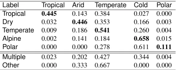
Table 4: Toponym mapping of resolved climate from the K¨oppen-Geiger climate map to the correspond-ing abstract’s gold standard climate label.

toponyms, but due to the sparsity of toponyms in the text, the loss of information from filtering out these resolutions outweighs any gain in precision from avoiding ambiguity in climate resolution.

In order to investigate how much of the problem could be attributed to incorrect disambiguation, a classifier with “oracle” toponym disambiguation is also tested. This oracle determined the propor-tion of instances in the dataset that had at least one climate resolution of a toponym that matches the gold standard label out of all the possible disam-biguations from the top 5 results of both DBpedia and GeoNames. The number of matches was only 2552 out of 3977 (64.2%) abstracts. This low per-centage suggests that the source of error cannot be primarily explained by toponym disambiguation. Another possible source of error for correctly dis-ambiguated toponyms is that the toponym is re-solved to the incorrect climate.

Based on the chosen set of label mappings, the distribution of resolved toponyms using the top result in DBpedia across the set of abstracts for each gold standard label was collected (Ta-ble 4). For each map label, the highest propor-tion of toponyms resolves to the expected dataset label. However, significant proportions are mis-matched in all cases. One cause of the poor accu-racy in climate resolution is that identifying cli-mate generally requires a greater degree of ge-ographic accuracy than resolving toponyms to a continent. Regions of continental scale generally contain more than one climatic zone (as seen in Figure 2). Therefore, coarse-grained toponyms representing countries or continents that provided valuable information in classification of study re-gion are no longer of use. The granularity filter classifiers were developed with the intention of filtering these out of the dataset. However, there was too much loss of information from the already

small number of available toponyms.

7 Conclusion

In this paper, we have explored NLP approaches to classifying climate type in environmental sci-ence abstracts based on resolving toponyms de-tected within the abstract to their climate type. This was done by first disambiguating the to-ponym with DBpedia and/or GeoNames to a set of geographic coordinates, then referencing the co-ordinates on a world map of climate classifica-tion. Supervised approaches with support vector machines also included features based on bag-of-words, bag-of-toponyms, and structural informa-tion. The classifiers developed in these experi-ments had limited success in outperforming base-line approaches. Bag-of-toponyms were demon-strated to be the most useful feature set, and the highest-performing classifier was DBpedia and GeoNames top-result toponym resolution in com-bination with bag-of-toponyms, achieving 0.695 classification accuracy.

Acknowledgments

NICTA is funded by the Australian Government as represented by the Department of Broadband, Communications and the Digital Economy and the Australian Research Council through the ICT Centre of Excellence program.

References

C.-C. Chang and C.-J. Lin. 2011. LIBSVM: A library for support vector machines. ACM Transactions on

Intelligent Systems and Technology, 2:27:1–27:27.

Software available athttp://www.csie.ntu. edu.tw/˜cjlin/libsvm.

G. Chung. 2009. Sentence retrieval for abstracts of randomized controlled trials. BMC Medical Infor-matics and Decision Making, 9(1):10.

J.R. Finkel, T. Grenager, and C. Manning. 2005. In-corporating non-local information into information extraction systems by Gibbs sampling. In Proceed-ings of the 43rd Annual Meeting on Association for

Computational Linguistics, pages 363–370, Ann

Ar-bor, USA.

A. Gaudinat and C. Boyer. 2002. Automatic extraction of MeSH terms from Medline abstracts. In Work-shop on Natural Language Processing in Biomedi-cal Applications, pages 53–57, Nicosia, Cyprus.

S. Kim, D. Martinez, L. Cavedon, and L. Yencken. 2011. Automatic classification of sentences to sup-port evidence based medicine. BMC Bioinformatics, 12(Suppl 2):S5.

S.E. Overell and S. R¨uger. 2006. Identifying and grounding descriptions of places. In3rd Workshop on Geographic Information Retrieval, Seattle, USA.

M.C. Peel, B.L. Finlayson, and T.A. McMahon. 2007. Updated world map of the K¨oppen-Geiger climate classification. Hydrology and Earth System

Sci-ences, 11:1633–1644.

D.L. Sackett, W. Rosenberg, JA Gray, R.B. Haynes, and W.S. Richardson. 1996. Evidence based medicine: what it is and what it isn’t. British Medi-cal Journal, 312(7023):71–72.

D. Santos and M.S. Chaves. 2006. The place of place in geographical IR. In3rd Workshop on Geographic Information Retrieval, Seattle, USA.

N. Stokes, Y. Li, A. Moffat, and J. Rong. 2008. An em-pirical study of the effects of NLP components on geographic IR performance. International Journal

of Geographical Information Science, 22(3):247–

264.

J.A. Webb, S.R. Wealands, P. Lea, S.J. Nichols, S.C. de Little, M.J. Stewardson, R.H. Norris, F. Chan, D. Marinova, and R.S. Anderssen. 2011. Eco Evidence: using the scientific literature to in-form evidence-based decision making in environ-mental management. In MODSIM2011 Interna-tional Congress on Modelling and Simulation, pages 2472–2478, Perth, Australia.

J.A. Webb, S.C. de Little, K.A. Miller, and M.J. Stew-ardson. 2012a. Eco Evidence Database: a dis-tributed modelling resource for systematic literature analysis in environmental science and management.

In 2012 International Congress on Environmental

Modelling and Software, pages 1135–1142, Leipzig,

Germany.

J.A. Webb, E.M. Wallis, and M.J. Stewardson. 2012b. A systematic review of published evidence link-ing wetland plants to water regime components.

Aquatic Botany, 103:1–14.

J. Willett, T. Baldwin, D. Martinez, and A. Webb. 2012. Classification of study region in environmen-tal science abstracts. In Proceedings of the Aus-tralasian Language Technology Association