(Analytic Formula for the European Normal Black Scholes Formula)

(Analytic Formula for the European Normal Black Scholes Formula)

by

Kazuhiro Iwasawa

December 2, 2001

In this short summary paper, a brief summary of Black Scholes type formulae for Normal model will be given. Usually the underlying security is assumed to follow a lognormal process (or Geometric Brownian Motion). However, there are some traders who believe that the normal process describes the real market more closely than that of lognormal counterpart. The derivation of the formula will be proved mathematically by the famous no-arbitrage argument (Hull[1]). Then, the Greeks (delta, gamma, theta, and vega) will be computed by differentiation.

The idea of the theory is that The fair value of any derivative security is computed as the expectation of the payoff under an equivalent martingale measure (Karatzas [2]). More specifically, the price is the expectation of a discounted payoff under the risk neutral measure. This measure (or density) is a solution to a parabolic partial differential equation driven by the underlying process (lognormal process). The detailed statements will be shown below. Section following the next will show arguments concerning Normal model that does not allow negative underlier price. Also brief experiments regarding how one can approximate lognormal Black Scholes with Normal version will be explored with some experiments.

1

Analytic Formula

Theorem 1 (Analytic Formula for a Normal Black Scholes Model)

Let us assume that the current future price, strike price, risk free interest rate, volatility, and time to maturity as denoted as F,K,r,σ, andT−trespectively. Alet us also assume that the current future price follows the following Normal process:

dF = µdt+σdWt (1)

whereµ is a constant drift.

Then, the fair values of callC and putP are expressed as :

C = e−r(T−t)[(F−K)N(d1) +σ

√

T−t

√

2π e

−d2₁/2

] (2)

and

P = e−r(T−t)[(K−F)N(−d1) +σ

√

T−t

√

2π e

−d2₁/2

] (3)

whered1=_σF√−K

T₋t

Moreover, the Greeks (delta, gamma, vega, theta) are computed by simple differentiation of the above formulas to give: (Note: Detail calculations will be shown below for more general audience)

Delta₍Call₎ =

∂C ∂F

= e−r(T−t)[(F−K)√1 2πe

−d2₁/₂ 1

σ√T−t]

+e−r(T−t)N(d1) +e−r(T−t)σ

√

T−t

√

2π e

−d2₁/2

[−(F−K)

σ√T−t][

1

σ√T−t]

= e−r(T−t)N(d₁) (4)

Delta₍P ut) =

∂P ∂F

= e−r(T−t)[(K−F)√1 2πe

−d2₁/2 −1

σ√T−t]

−e−r(T−t)N(−d₁) +e−r(T−t)σ

√

T−t

√

2π e

−d2₁/₂

[−(F−K)

σ√T−t][

1

σ√T−t]

= −e−r(T−t)N(−d₁) (5)

Gamma₍Call₎=Gamma₍P ut₎ =

∂2C ∂F2(∗)

= e−r(T−t)√1

2πe

−d2₁/₂ 1

σ√T−t

= e

−r₍T₋t₎

σ√T−t

1

√

2πe

−d2₁/2

(6)

( *Note: This is evident from the Put-Call parity in that by differentiating the Put-Call parity formula twice with respect to the underlier establishes the equality of Put and Call for all option models ..)

V ega₍Call)=V ega(P ut) =

∂C ∂σ

= e−r(T−t)(F−K)√1 2πe

−d2₁/2

[−(F−K)

σ2√T−t]

+e−r(T−t)

√

T−t

√

2π e

−d2₁/2

+e−r(T−t)σ

√

T−t

√

2π e

−d2₁/2

[−(F−K)

σ√T−t][−

(F−K)

σ2√T−t]

= e−r(T−t)

√

T−t

√

2π e

−d2₁/₂

(7)

T heta₍Call) =

∂C ∂t

= −re−r(T−t)[(F−K)N(d₁) +σ

√

T −t

√

2π e

−d2₁/₂

]

−e−r(T−t)[(F−K)√1 2πe

−d2₁/2

(−1 2

F−K σ(T−t)3/2)] −e−r(T−t)[ σ

2√2πte

−d2₁/₂

]

−e−r(T−t)[σ

√

T−t

√

2π e

−d2₁/2

(−(F−K)

σ√T−t)(−

(F−K) 2σ(T−t)3/2)]

= −re−r(T−t)[(F−K)N(d₁) +σ

√

T −t

√

2π e

−d2₁/2

]

−e−r(T−t)[ σ 2√2πte

−d2₁/₂

] (8)

T heta₍P ut₎ =

∂P ∂t

= −re−r(T−t)[(K−F)N(−d₁) +σ

√

T−t

√

2π e

−d2₁/₂

]

−e−r(T−t)[(K−F)√1 2πe

−d2₁/₂

(−1 2

F−K σ(T −t)3/2)] −e−r(T−t)[ σ

2√2πte

−d2₁/₂

]

−e−r(T−t)[σ

√

T−t

√

2π e

−d2₁/₂

(−(F−K)

σ√T−t)(−

(F−K) 2σ(T −t)3/2)]

= −re−r(T−t)[K−F)N(−d₁) +σ

√

T−t

√

2π e

−d2₁/2

]

−e−r(T−t)[ σ 2√2πte

−d2₁/₂

] (9)

(Proof)

We shall parallel the argument given in Hull [1]. The proof will be heuristic. Let us study the behavior of the delta hedged portfolio which consists of long delta shares of future contract and short one derivative in question. Say, call it Π. Let us also denote the value of derivative byg. Then, the value of the delta hedged portfolio is given by:

Π = g− ∂g

∂FF (10)

∆Π = ∆g− ∂g ∂F∆F

= (∂g

∂t + ∂g ∂Fµ+

1 2

∂2g ∂F2σ

2_)∆t+ ∂g

∂Fσ∆Wt

−∂g

∂F(µ∆t+σ∆Wt) (11)

= (∂g

∂t +

1 2

∂2g ∂F2σ

2_)∆t

We want the avove quantity to be a martingale under the discounted expectation with risk free rate. This is essentially the same as stating that the above quantity equals the gain from the risk free interest rate for the portfolio value. So, we have:

∆Π = rΠ∆t (12)

Since it cost nothing to enter into a futures contract, one has:

Π = g (13)

Thus we have:

(∂g

∂t +

1 2

∂2g ∂F2σ

2_{)∆t = rg∆t (14)}

Therefore, we obtains the following parabolic PDE:

∂g ∂t +

1 2

∂2g ∂F2σ

2 _{= rg (15)}

So, if the terminal payoff is given by g(T, F) = f(F), then by the application of Feynman-Kac (see Karatzas and Shrieve[2]), one obtains the following solution:

g(t, x) = Ex[e−r(T−t)f(y)]

= e

−r(T−t)

σ√T−t√2π

_∞

−∞f(y)e

−_2σ(x₂₍−_Ty)2_−t)

dy (16)

where

f(y) =

(y−K)+ for Call (K−y)+ for Put.

Therefore, the for the formula for the above can be simplifed by simply expanding the expression inside the integral. The detail will be shown for more general audience.

Call = g(t, F)

= EF[e−r(T−t)f(y)]

= e

−r₍T₋t₎

σ√T−t√2π

_∞

−∞(y−K)

+_e−2(σF2(−Ty−)2t)_dy

= e

−r₍T₋t₎ √

2π

_∞

−∞(F+σ

√

T−t x−K)+e−x22_dx

= e

−r(T−t) √

2π

_∞

(K−F)

σ√T−t

(F+σ√T−t x−K)e−x22_dx

= e

−r(T−t) √

2π

_∞

(K−F)

σ√T−t

(F−K)e−x22_dx

+ e

−r(T−t) √

2π

_∞

(K−F)

σ√T−t

(σ√T−t x)e−x22_dx

= e−r(T−t)[(F−K)N(d1) +σ

√

T−t

√

2π e

−d2₁/2

] (17)

whered1=_σF√−K

T₋t

Similarly for the put, we have:

P ut = g(t, F)

= EF[e−r(T−t)f(y)]

= e

−r₍T₋t₎

σ√T−t√2π

_∞

−∞(K−y)

+_e−2(σF2(−Ty−)2t)_dy

= e

−r₍T₋t₎ √

2π

_∞

−∞(K−F−σ

√

T−t x)+e−x22_dx

= e

−r(T−t) √

2π

(K−F)

σ√T−t

−∞ (K−F−σ

√

T−t x)e−x22_dx

= e

−r₍T₋t₎ √

2π

(K−F)

σ√T−t

−∞ (K−F)e −x2

2 _dx

+ e

−r(T−t) √

2π

(K−F)

σ√T−t

−∞ (−σ

√

T−t x)e−x22_dx

= e−r(T−t)[(K−F)N(−d₁) +σ

√

T−t

√

2π e

−d2₁/₂

] (18)

whered₁ is defined similarly as in (17).

This is what we need to prove. The Greeks are obtained by simple differentiations which are worked out in the statement of the theorem.

2

Normal Process under the Bounded Negative Assumption

In the previous section, pricing scheme for the Normal Process is proved in more general setting. That is the underling prices are allowed to become negative. In this section, the modified option formulas will be derived where underlier price can not fall below certain number, say−R.

Using the same notations as in the previous section, we have the following PDE for non negative underlier process.

∂g ∂t +

1 2

∂2g ∂F2σ

2 _{= rg}

g(T, F) = f(F)

F ≥ −R (19)

This is a problem constrained in the half plane inF axis. The solution of the above PDE can be solved by transforming the above PDE into a typical PDE problem for the entireF axis. This is done by extend-ing the terminal functionf(F) intof−R(F) which is basically an odd extention of the original functionf(F).

Thus, the unique solution exists for this PDE (John [4]), and given by:

g(t, x) = Ex[e−r(T−t)f(y)]

= e

−r₍T₋t₎

σ√T −t√2π

_∞

−∞f−R(y)e − (x−y)2

2σ2(T−t)_dy

= e

−r₍T₋t₎

σ√T −t√2π

_∞

−R

f(y)[e−

(x−y+R)2 2σ2(T−t) −_e−

(x+y−R)2

2σ2(T−t)_{]dy (20)}

where

f(y) =

(y−K)+ for Call (K−y)+ for Put.

Therefore the formula for the Call option is given by expanding the messy expression in (20) as:

Call = g(t, F)

= EF[e−r(T−t)f(y)]

= e

−r(T−t)

σ√T−t√2π

_∞

−∞f−R(y)e

− (F−y)2 2σ2(T−t)_dy

= e

−r₍T₋t₎

σ√T−t√2π

_∞

−R

f(y)[e−

(F−y+R)2

2σ2(T−t) −_e−(2Fσ+2(yT−−Rt)2) _]dy

= e

−r₍T₋t₎

σ√T−t√2π

_∞

−R

(y−k)+[e−

(F−y+R)2 2σ2(T−t) −_e−

(F+y−R)2 2σ2(T−t) _]dy

= e

−r(T−t) √

2π

_∞

(K−F−R)

σ√T−t

(F+σ√T−t x+R−K)+e−x22_dx

+e

−r(T−t) √

2π

_∞

(K+F−R)

σ√T−t

(−F−σ√T−t z+R−K)e−z22_dz

= e−r(T−t)[(R+F−K)N(d₁) +σ

√

T−t

√

2π e

−d2₁/₂

−e−r(T−t)[(R−F−K)N(d₂) +σ

√

T−t

√

2π e

−d2₂/2

] (21)

whered₁=R_σ+√F−K

T−t , andd2=

R₋F₋K σ√T−t

Similarly for put, we have:

P ut = g(t, F)

= EF[e−r(T−t)f(y)]

= e

−r(T−t)

σ√T−t√2π

_∞

−∞f−R(y)e

− (F−y)2 2σ2(T−t)_dy

= e

−r₍T₋t₎

σ√T−t√2π

_∞

−R

f(y)[e−

(F−y+R)2

2σ2(T−t) −_e−(2Fσ+2(yT−−Rt)2) _]dy

= e

−r₍T₋t₎

σ√T−t√2π

_∞

−R

(k−y)+[e−

(F−y+R)2 2σ2(T−t) −_e−

(F+y−R)2 2σ2(T−t) _]dy

= e

−r(T−t) √

2π

(K−F−R)

σ√T−t

−∞ (K−F−σ

√

T−t x−R)+e−x22_dx

+e

−r₍T₋t₎ √

2π

_∞

(K+F−R)

σ√T−t

(K+F−σ√T−t z−R)e−z22_dz

= e−r(T−t)[(K−F−R)N(d1) +σ

√

T−t

√

2π e

−d2₁/2

]

−e−r(T−t)[(K+F−R)N(d₂) +σ

√

T−t

√

2π e

−d2₂/2

] (22)

whered₁=R_σ+√F−K

T−t , andd2=

R₋F₋K σ√T−t

Let us compare the result with the results from the previous section. LetingR= 0 in the expression (21) gives:

Call = e−r(T−t)[(F−K)N(d1) +σ

√

T−t

√

2π e

−d2₁/2

]

−e−r(T−t)[(−F−K)N(d₂) +σ

√

T−t

√

2π e

−d2₂/2

] (23)

whered₁=_σF√−K

T−t, andd2=

−F₋K σ√T−t

Sinced₂ term is such a large negative quantity, the term−e−r(T−t)_{[(−F−K)N(d}

2) + σ

√

T−t

√

2π e

−d2₂/2_{] is}

a very small quantity.

Thus, the call price becomes:

Call ≈ e−r(T−t)[(F−K)N(d1) +σ

√

T−t

√

2π e

−d2₁/2

] (24)

Actually, the the second term is so small that one can replace the above relation with equality in most practical cases. The identical argument can be made for the put as well.

The above price have a very nice theoretical property whenσ is extremely large. The expressions (2) and (3) blows up to infinity when we letσ→ ∞

Without the loss of generality, let us assume R = 0 as before. Then taking the limit of the expression (21) gives:

lim

σ→+∞Call = σ→lim+∞e

−r(T−t)

[(F−K)N(d₁) +σ

√

T−t

√

2π e

−d2₁/2

]

lim

σ_→+∞−e

−r₍T₋t₎

[(−F−K)N(d₂) +σ

√

T−t

√

2π e

−d2₂/₂

]

= e−r(T−t)(F−K) + lim

σ_→+∞e

−r₍T₋t₎σ √

T−t

√

2π [e

−d2₁/₂₋

e−d22/2_]

= e−r(T−t)(F−K) + lim

σ→+∞e

−r₍T₋t₎σ √

T−t

√

2π [

∞

n=1

((−₂₍(F_T−₋K_t))2)n−(−₂₍(F_T+₋K_t))2)n)

σ2n_n! ]

= e−r(T−t)(F−K) (25)

Similarly for put, we have:

lim

σ_→+∞P ut = e

−r₍T₋t₎

(K−F) (26)

3

Approximation Experiments

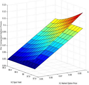
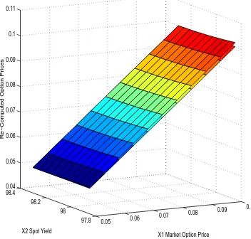
In practice, option prices are given in the market and one ends up computing implied volatility for a particular option. Suppose one is given an implied volatility for the lognormal model but wants to use normal model to compute its greeks (delta, gamma, vega, and theta). This is usually dealt with approximatingσ₍N ormal)

by letting σ₍N ormal) = ˆGσ(Lognormal), Where ˆG is a scaling constant. What kind approximations can one

make? The popular choice is to set ˆG=K(strike), or ˆG=F (future price). Then use these into the Normal model. These approximations display reasonable closeness to the actual lognormal price. Brief experiments have shown that taking the average of these two ˆG= (F+K)/2 gives very approximation to the lognormal price. Since, this paper is intended to be a very short paper, brief explanation of the experiments with some graphs would be shown below.

0.05 0.06

0.07 0.08

0.09 0.1

97.8 97.9 98 98.1 98.2 98.3 0.04 0.05 0.06 0.07 0.08 0.09 0.1 0.11 0.12 0.13

X1 Market Option Price Eurodollar Future Option Price Analysis (Using Spot as Scaling)

X2 Spot Yield

Re−Computed Option Prices

0.05 0.06

0.07 0.08

0.09 0.1

97.8 97.9 98 98.1 98.2 98.3 0.03 0.04 0.05 0.06 0.07 0.08 0.09 0.1 0.11

X1 Market Option Price Eurodollar Future Option Price Analysis (Using Strike as Scaling)

X2 Spot Yield

Re−Computed Option Prices

0.05 0.06 0.07

0.08 0.09 0.1

97.8 98

98.2 98.4

0.04 0.05 0.06 0.07 0.08 0.09 0.1 0.11

X1 Market Option Price Eurodollar Future Option Price Analysis (Using (Strike + Spot)/2 as Scaling)

X2 Spot Yield

Re−Computed Option Prices

0.05

0.06

0.07

0.08

0.09

0.1 _97.8

97.9 98

98.1

98.2

98.3 −1.8

−1.6 −1.4 −1.2 −1 −0.8 −0.6 −0.4 −0.2 0

x 10−3

X2 Spot Yield Eurodollar Future Option Price Error Analysis

X1 Market Option Price

Error

References

[*]

[1] Hull, J. (1993), Options, Futures, and Other Derivative Securities, 2nd Edition, Prentice Hall. [2] Karatzas, I. and S.E. Shreve (1988), Brownian Motion and Stochastic Calculus,Springer-Verlag, New York.

[3] Press, W.H., Teokolsky, S.A., Vetterling, W.T. and Flannery, B.P. (1992), Numerical Reciepes in C: The Art of Scientific Computing, 2nd Edition, Cambridge University Press, Cambridge