60
Udham Singh Nagar District, Uttarakhand
Arvind Singh Tomar
1, Praveen Vikram Singh
2, Om Prakash Kumar
31Department of Irrigation & Drainage Engineering, 2Department of Soil & Water Conservation Engineering, College of Technology, Govind Ballabh Pant University of Agriculture & Technology,
Pantnagar (Uttarakhand) 263145 Email: arvindstomar@gmailcom1
Abstract- In this study, the variation in rainfall pattern and its distribution at Udham Singh Nagar district of
Uttarakhand was analyzed on the basis of long-term rainfall dataset of 53 years (1961-2013) recorded at the Govind Ballabh Pant University of Agriculture & Technology, Pantnagar. The analysis revealed high magnitude of rainfall dissimilarity as it varied in between 3.89-430.33 mm and 775.70-3218.60 mm on monthly and annual basis respectively. The analysis stressed out need to construct water harvesting bodies to utilize stored rainwater for growing crops during water stressed periods in the Udham Singh Nagar district of Uttarakhand.
Index Terms- Rainfall; departure; statistical.
1. INTRODUCTION
Water is becoming a scarce resource as a result of growing demand for its various uses e.g. hydropower, irrigation, water supply etc. It is the most limiting natural resource which can hinder economic development of any country and its availability at correct time in adequate quantity is one of the important factors which influence crop yields. The marginal and small farmers constituting 80% of agricultural income group still depend on rainfed farming. Throughout much of the world, irrigation is supplemental to rainfall which is the important factor to support life and produce food. Due to increasing population and developmental changes, over-exploitation of natural resources resulting in degraded land, reduced water availability and changed climatic conditions.
The non-availability of certain amount of rainfall, a continuous random variable at critical period can influence failure of various agricultural related issues. The determination of rainfall amount and its behaviour over time and space has many practical applications in engineering and agriculture. In designing and operation of irrigation systems, it is becoming increasingly important to account the contribution made by natural rainfall in crop production as it can contribute significantly to crop water requirements. The early or delay in onset monsoon and withdrawal of monsoon, breaks in monsoon period and unusual heavy rainfall may disturb normal crop growth and its development.
To utilize available rainfall effectively, crop planning and management practices must be followed based on amount and distribution of rainfall at a place. The production of agricultural crops can be significantly increased with proper management of rainwater and
timely application of optimum irrigation water. In our country, rainfall distribution is very erratic in nature and varies from region to region and year to year though adequate rainfall is received through four different types of weather phenomenon namely, south-west monsoon (about 74%), north-east monsoon (about 3%), pre-monsoon (about 13%) and post-monsoon (about 10%) with an average annual rainfall as 119 cm. In Indian conditions, existing uncertainty in availability of water throughout the year can be effectively balanced by creating water storage reservoirs. A number of research workers have analyzed rainfall behaviour for various purposes. The fluctuation in rainfall at different timescales was analysed by [1]-[13], whereas, on statistical basis, it has been evaluated by [14]-[18] with different mathematical formulae presented in [19].
2. MATERIALS AND METHODS
The long-term daily rainfall data of Udham Singh Nagar district of Uttarakhand for a period of 53 years (1961-2013) collected from the Meteorological observatory situated at Crop Research Centre of G.B. Pant University of Agriculture & Technology, Pantnagar was analyzed by using mathematical and statistical techniques. The mathematical procedure involved determination of mean value of rainfall on monthly, seasonal and annual basis to evaluate its departure in order to understand its pattern. The values of mean, median, mode, dispersion, standard deviation and coefficients of Dispersion, Variation, Skewness and Kurtosis were computed as a part of statistical analysis.
3. RESULTS AND DISCUSSIONS
Mathematical analysis: The most commonly used
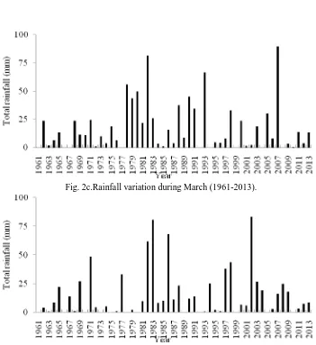
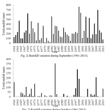
61 (year 1991) for January, February, March, April, May, June, July, August, September, October, November and December respectively. The average monthly and seasonal rainfall data of study area is presented in Table 1. The values of mean monthly rainfall is being exhibited in Fig. 1, whereas, its variation for all the 12 months (January-December), three seasons (monsoon, winter and summer) and different years is presented in Figs. 2a-l, 2m-o and 2p respectively.
The maximum rainfall during monsoon, winter and summer seasons was recorded as 2232.80 mm, 230.40 and 905.00 mm in years 1999, 1961 and 2000 respectively, whereas, their respective minimum values were recorded as 398.20 mm (year 1979), 5.02 mm (year 2008) and 32.40 mm (year 2012). The monthly, seasonal (monsoon, winter, summer) and annual basis is shown in Figs. 3a-l, 3m-o, and 3p respectively.
The information regarding different years receiving more or less than mean rainfall on monthly basis rainfall were observed during October (42) followed by November (41). From Table 2, it can be inferred that out of 53 years, 34, 30, 30 and 33 years received less than mean monthly rainfall during the months of June, July, August and September respectively.
The average annual rainfall of Udham Singh Nagar district during study period (1961-2013) was obtained as 1499.62 mm. The graph (Fig. 2m) shows downside departure from average annual rainfall during years 1962, 1963, 1965, 1966, 1967, 1969, 1970, 1972, 1974, 1975, 1977, 1978, 1979, 1980, 1981, 1987, 1989, 1991, 1992, 1993, 1994, 1995, 1996, 1997, 2004, 2006, 2009 and 2012 shows requirement of groundwater extraction for various uses. The trend of annual departure reveals that years showing annual departure more than long-term mean annual rainfall were 1961, 1964, 1968, 1971, 1973, 1976, 1982, 1983, 1984, 1985, 1986, 1988, 1990, 1998, 1999,
2000, 2001, 2002, 2003, 2005, 2007, 2008, 2010, 2011 and 2013. Hence, these years were found favourable for groundwater recharging.
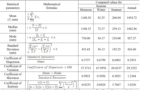
Statistical analysis: The statistical method employed
for analyzing rainfall data of study area includes determination of mean, median, mode, standard deviation, coefficients of Dispersion, Variation, Skewness and Kurtosis and pertinent results are presented in Table 3. The statistical analysis of annual rainfall data reveals that mean annual rainfall of area is 1454.72 mm, whereas, computed value of median (1442.86 mm) and mode (927.27 mm) indicates ideal rainfall. The calculated value of Standard Deviation reveals that deviation of rainfall is 426.60 mm over a period of 53 years. The coefficient of variation indicates that amount of rainfall varies up to 29.325 with coefficient of Skewness (1.2364) showing positive trend, whereas, coefficient of kurtosis (1.0236) confirms that annual distribution is relatively a peaked one. rainfall variation on monthly, seasonal and annual basis in recharge phenomena of groundwater system in Udham Singh Nagar district of Uttarakhand is being presented in this paper.
REFERENCES Invercargill, New Zealand, New Zealand Journal of Geology and Geophysics, 31: 247-256.
[3] Essery, C. I.; Wilcock, D. N. (1991): The variation in rainfall catch from standard UK Meteorological Office raingauges: A twelve year case study, Hydrological Sciences Journal,
36(1): 23-34.
[4] Kunkel, K. E.; Andsager, K.; Easterling, D. R. (1999): Long-term trends in extreme precipitation events over the Conterminous United States and Canada, Journal of Applied Meteorology, 12: 2515-2527.
[5] Garreaud, R. D. (2000): Intraseasonal variability of moisture and rainfall over the South American Altiplano, Monthly Weather Review, 128: 3337-3346.
62 total and variability (1970–2000) along the
Kwazulu-Natal Drakensberg Foothills. South African Geographical Journal, 88(2): 130-137. [8] Tomar, A. S. (2006): Rainfall analysis for
ensuring soil moisture availability at dryland areas of semi-arid Indore region of Madhya Pradesh, Journal of Soil and Water Conservation,
5(1): 1-5.
[9] Vennila, G.; Subramani, T.; Elango, L. (2007). Rainfall variation analysis of Vattamalaikarai sub-basin, Tamilnadu, India, Journal of Applied Hydrology, XX(3): 50-59.
[10]Kwarteng, A. Y.; Dorvlob, A. S.; Vijaya Kumar, G. T. (2009): Analysis of a 27-year rainfall data (1977–2003) in the Sultanate of Oman, International Journal of Climatology, 29: 605– 617.
[11]Kumar, V.; Jain, S. K.; Singh, Y. (2010): Analysis of long-term rainfall trends in India, Hydrological Sciences Journal, 55(4): 484-496. [12]Caloiero, T.; Coscarelli, R.; Ferrari, E.; Mancini,
M. (2011): Trend detection of annual and seasonal rainfall in Calabria (Southern Italy), International Journal of Climatology 31: 44–56. [13]Wagesho, N.; Goel, N. K.; Jain, M. K. (2013),
Temporal and spatial variability of annual and seasonal rainfall over Ethiopia, Hydrological Sciences Journal, 58(2): 354-373.
[14]Unkasevic, M.; Radinovic, D. (2000): Statistical analysis of daily maximum and monthly precipitation at Belgrade, Theoretical Applied Climatology, 66(3-4): 241-249.
[15]Seetharam, K. (2003): Correlation structure of daily rainfall over Teesta catchment, Mausam,
54(2): 447-452.
[16]Basu, G. C.; Bhattacharjee, U.; Ghosh, R. (2004): Statistical analysis of rainfall distribution and trend of rainfall anamolies district wise during monsoon period over West Bengal, Mausam,
55(3): 409-418.
[17]Kim, D.; Olivera, F. (2012): Relative importance of the different rainfall statistics in the calibration of stochastic rainfall generation models, Journal of Hydrologic Engineering, 17(3): 368–376. [18]Maftei, C.; Barbulescu, A. (2012). Statistical
analysis of precipitation time series in Dobrudja region, Mausam, 63(4): 553-564.
65 Table 2: Years receiving excess and deficit rainfall in comparison to mean monthly rainfall (1961-2013).
Months Years receiving rainfall
More than mean monthly rainfall Less than mean monthly rainfall
January
1961, 1962, 1968, 1970, 1971, 1975, 1979, 1981, 1982, 1983, 1989, 1994, 1995, 1996, 1999, 2002, 2003, 2005, 2013
1963, 1964, 1965, 1966, 1967, 1969, 1972, 1973, 1974, 1976, 1977, 1978, 1980, 1984, 1985, 1986, 1987, 1988, 1990, 1991, 1992, 1993, 1997, 1998, 2000, 2001, 2004, 2006, 2007, 2008, 2009, 2010, 2011, 2012
February
1961, 1965, 1971, 1972, 1976, 1978, 1979, 1984, 1986, 1990, 1991, 1994, 1996, 2000, 2002, 2003, 2005, 2007, 2013
1962, 1963, 1964, 1966, 1967, 1968, 1969, 1970, 1973, 1974, 1975, 1977, 1980, 1981, 1982, 1983, 1985, 1987, 1988, 1989, 1992, 1993, 1995, 1997, 1998, 1999, 2001, 2004, 2006, 2008, 2009, 2010, 2011, 2012
March
1962, 1968, 1971, 1975, 1978, 1979, 1980, 1981, 1982, 1983, 1988, 1990, 1991, 1993, 1998, 2000, 2003, 2005, 2007
1961, 1963, 1964, 1965, 1966, 1967, 1969, 1970, 1972, 1973, 1974, 1976, 1977, 1984, 1985, 1986, 1987, 1989, 1992, 1994, 1995, 1996, 1997, 1999, 2001, 2002, 2004, 2006, 2008, 2009, 2010, 2011, 2012, 2013
April
1965, 1969, 1971, 1977, 1982, 1983, 1986, 1988, 1994, 1997, 1998, 2002, 2003, 2004, 2007, 2008, 2009
1961, 1962, 1963, 1964, 1966, 1967, 1968, 1970, 1972, 1973, 1974, 1975, 1976, 1978, 1979, 1980, 1981, 1984, 1985, 1987, 1989, 1990, 1991, 1992, 1993, 1995, 1996, 1999, 2000, 2001, 2005, 2006, 2010, 2011, 2012, 2013
May
1970, 1971, 1973, 1976, 1977, 1981, 1982, 1985, 1986, 1987, 1990, 1998, 1999, 2000, 2001, 2003, 2004, 2006, 2010, 2011
1961, 1962, 1963, 1964, 1965, 1966, 1967, 1968, 1969, 1972, 1974, 1975, 1978, 1979, 1980, 1983, 1984, 1988, 1989, 1991, 1992, 1993, 1994, 1995, 1996, 1997, 2002, 2005, 2007, 2008, 2009, 2012, 2013
June
1962, 1966, 1973, 1975, 1976, 1979, 1980, 1982, 1984, 1989, 1999, 2000, 2001, 2002, 2003, 2007, 2008, 2011, 2013
1961, 1963, 1964, 1965, 1967, 1968, 1969, 1970, 1971, 1972, 1974, 1977, 1978, 1981, 1983, 1992, 1993, 1994, 1995, 1996, 1997, 1998, 2000, 2001, 2002, 2004, 2006, 2009, 2012, 2013
August
1961, 1963, 1967, 1971, 1973, 1976, 1982, 1983, 1985, 1995, 1998, 1999, 2000, 2001, 2002, 2003, 2004, 2005, 2007, 2008, 2010, 2011, 2013
1962, 1964, 1965, 1966, 1968, 1969, 1970, 1972, 1974, 1975, 1977, 1978, 1979, 1980, 1981, 1984, 1986, 1987, 1988, 1989, 1990, 1991, 1992, 1993, 1994, 1996, 1997, 2006, 2009, 2012
September
1964, 1968, 1969, 1971, 1972, 1975, 1978, 1983, 1985, 1986, 1987, 1990, 1999, 2000, 2002, 2003, 2005, 2008, 2010, 2011
1961, 1962, 1963, 1965, 1966, 1967, 1970, 1973, 1974, 1976, 1977, 1979, 1980, 1981, 1982, 2000, 2001, 2002, 2003, 2004, 2005, 2006, 2007, 2008, 2010, 2011, 2012
November
1963, 1971, 1972, 1979, 1981, 1989, 1991, 1992, 1997, 1998, 2001, 2009
1961, 1962, 1964, 1965, 1966, 1967, 1968, 1969, 1970, 1973, 1974, 1975, 1976, 1977, 1978, 1980, 1982, 1983, 1984, 1985, 1986, 1987, 1988, 1990, 1993, 1994, 1995, 1996, 1999, 2000, 2002, 2003, 2004, 2005, 2006, 2007, 2008, 2010, 2011, 2012, 2013
December
1961, 1964, 1967, 1974, 1977, 1980, 1981, 1982, 1984, 1985, 1986, 1990, 1991, 1997, 1999, 2003, 2010
66 Table 3: Statistical parameters of rainfall on seasonal and annual basis (1961-2013).
Statistical
Dispersion 0.3737 0.6799 0.6963 0.2933
Coefficient of
Variation 37.3715 67.9976 69.6337 29.3252
Coefficient of
Skewness 0.9925 0.5056 0.3025 1.2364
Coefficient of
Kurtosis -0.0233 0.0424 3.7667 1.0236
= mean; N = total frequency; C = cumulative frequency of group preceding the median group; l = lower limit of modal class; fm = maximum frequency; f1, f2 = frequencies of classes preceding and following modal
70 Fig. 2c.Rainfall variation during March (1961-2013).
71 Fig. 2e.Rainfall variation during May (1961-2013).
72 Fig. 2g.Rainfall variation during July (1961-2013).
73 Fig. 2i.Rainfall variation during September (1961-2013).
74 Fig. 2k.Rainfall variation during November (1961-2013).
75 Fig. 2m.Rainfall variation during monsoon season (1961-2013).
76 Fig. 2o.Rainfall variation during summer season (1961-2013).
77 Fig. 3a.Departure from mean rainfall in January (1961-2013).
78 Fig. 3c.Departure from mean rainfall in March (1961-2013).
79 Fig. 3e.Departure from mean rainfall in May (1961-2013).
80 Fig. 3g.Departure from mean rainfall in July (1961-2013).
81 Fig. 3i.Departure from mean rainfall in September (1961-2013).
82 Fig. 3k.Departure from mean rainfall in November (1961-2013).
83 Fig. 3m.Departure from mean monsoon rainfall (1961-2013).
84 Fig. 3o.Departure from mean summer rainfall (1961-2013).